“What” and “Where” in auditory sensory processing: a high-density electrical mapping study of distinct neural processes underlying sound object recognition and sound localization

Introduction

There is growing evidence for functionally and anatomically distinct auditory processing pathways. Findings in non-human primates (Romanski et al., 1999; Rauschecker and Tian, 2000; Tian et al., 2001) and humans (Weeks et al., 1999; Clarke et al., 2000, 2002; Anourova et al., 2001; Zatorre et al., 2002; Poremba et al., 2003) point to a WHAT/WHERE distinction analogous to that seen in the visual system (Mishkin et al., 1982). These data suggest a system whereby auditory inputs are communicated dorsally from primary auditory cortex for the extraction of information regarding spatial localization in parietal cortical regions (the WHERE pathway), and ventrally from primary auditory cortex along medial and inferior temporal cortex for the processing of the specific object features of the signal such as spectral content and temporal integration (the WHAT pathway).

Much of what we know about WHAT and WHERE auditory pathways comes from studies in non-human primates, which suggest that the earliest evidence for separable and functionally distinct pathways can already be found in the medial geniculate nucleus (MGN) of the thalamus (Kaas and Hackett, 1999; Romanski et al., 1999; Rauschecker and Tian, 2000). Rauschecker and Tian (2000) summarized work utilizing histochemical techniques and anatomical tracer dyes to track the trajectory of neuronal subpopulations from the MGN to primary auditory cortex (A1). Adjacent to A1 are a rostral area (R) and a caudomedial area (CM; Figure 1). While A1 and R have been shown to receive input from the ventral portion of the MGN, CM is the target of dorsal, and medial divisions of MGN. The lateral belt areas receiving input from A1 and R may represent the beginning of an auditory pattern or object stream, as the neurons here respond to species-specific vocalizations and other complex sounds (Romanski et al., 1999; Rauschecker and Tian, 2000). Conversely, neurons in caudal regions CM and CL (caudomedial and caudolateral regions respectively) show a good degree of spatial selectivity (see Tian et al., 2001). Romanski et al. (1999) traced the streams further in rhesus monkeys, finding distinct targets for the ventral and dorsal pathways in non-spatial and spatial domains of prefrontal cortex, respectively. Similarly, human lesion studies have provided additional support for the division of the auditory system into dorsal and ventral pathways with clear functional dissociations seen for patients with dorsal versus ventral lesions (Clarke et al., 2000, 2002; Clarke and Thiran, 2004).

FIGURE 1

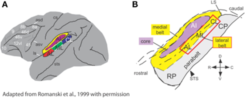
Figure 1. Anatomical regions of non-human primate (monkey) brain involved in processing of spatial and non-spatial stimuli. (A) Lateral belt region (in color) comprises A1, primary auditory cortex; CL, caudolateral belt region; AL, anterolateral belt region; ML, medial lateral belt region. (B) The same region, enlarged to show the locations of the medial and lateral belt (yellow), primary auditory cortex (purple) and the parabelt cortex on the superior temporal gyrus. Adapted from Romanski et al. (1999), with permission.

In humans, there is also mounting functional evidence for WHAT and WHERE divisions of the auditory system. Arnott et al. (2004) compiled a meta-analysis of neuroimaging studies of ventral and dorsal auditory processing in humans. By reviewing 11 spatial studies and 27 non-spatial studies, these authors concluded that physiologically distinct areas for processing spatial and non-spatial features of sounds could be identified. For the studies classified as “spatial,” centers of activation clustered around the inferior parietal lobule, the temporal lobe posterior to primary auditory cortex, and the superior frontal sulcus. For the non-spatial studies, centers of activation were seen clustered around inferior frontal cortex. While there was substantial overlap in areas of activation, the clusters of activation corresponded well with the notion that WHERE processing occurs in a dorsally positioned processing stream and WHAT processing in a ventrally positioned processing stream (see Figure 2). The studies included in this analysis all utilized positron emission tomography (PET) and/or functional magnetic resonance imaging (fMRI). Thus far, however, there have been relatively few electroencephalographic (EEG)/magnetoencephalographic (MEG) investigations of processing within these pathways in the human auditory system. Therefore, while we have some idea of the anatomical localization of the processing of these distinct types of information, our understanding of the temporal dynamics of these processes is still quite sparse.

FIGURE 2

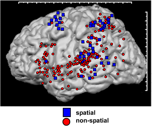
Figure 2. Schematic representation of auditory pathways as evidenced by a meta-analysis of 11 spatial (dorsal) and 27 non-spatial (ventral) studies. Regions showing greatest activation in each study are indicated. Adapted from Arnott et al. (2004) with permission.

Furthermore, the paradigms that have been employed to tap into functional capacities of auditory processing have varied greatly. For instance, a large portion of the non-spatial studies examined in the Arnott meta-analysis used human speech sounds, and this may be problematic insofar as speech represents a highly specialized auditory information class for humans, with a specific set of speech processing regions that may not necessarily lend themselves easily to this dorsal/ventral distinction. It has also been proposed that the dorsal pathway in humans not only processes auditory space, but also plays an important role in speech perception (Belin and Zatorre, 2000), raising the issue of possible overlap of presumptive dorsal and ventral pathway functions.

Human EEG and MEG studies have certainly attempted to shed some light on the timing of dorsal/ventral processing dissociations, but the findings have been highly inconsistent in terms of how early in the processing hierarchy information begins to be preferentially processed by a specific pathway. In the context of a match-to-sample task for location (right and left) and frequency (220, 440, and 880 Hz) that varied by memory load, Anurova et al. (2003) found very late effects of task differences occurring approximately 400 ms after stimulation. In an fMRI/EEG study, Alain et al. (2001) also found late occurring task-related effects from 300 ms onwards using a match-to-sample task. Stimuli in their study were five pitch-varied noise bursts delivered via headphones to five simulated spatial locations. In contrast to these findings of late processing differences, Anourova et al. (2001) using simultaneously recorded EEG and MEG, found peak latency differences between WHAT and WHERE tasks at considerably earlier time-points during the so-called N1 component of the AEP (∼100 ms), but there were no amplitude differences seen. In that study, identical blocks of tone stimuli were presented to subjects who were instructed to attend either to sound location or frequency. Stimuli were simple tones of two frequencies (1000 and 1500 Hz) delivered via headphones to two simulated locations (an interaural intensity difference was applied; perceived location was either left or right). Utilizing MEG and fMRI and a match-to-sample task with speech stimuli, Ahveninen et al. (2006) found both amplitude and latency effects at ∼70–150 ms (during the N1 component). De Santis et al. (2007a) also argued for “WHAT/WHERE” related effects on the amplitude of the auditory N1, but it is important to point out that in this study, subjects were involved in a passive listening task and did not explicitly perform spatial or object judgments. Stimuli were bandpass filtered noise bursts (250 or 500 Hz) delivered to two perceived locations (interaural time difference was used to simulate left and right locations). Although the aim of this study was for a setup where the stimuli used in the WHAT and WHERE conditions were “identical,” this was not in fact the case, and the design resulted in unique stimulus configurations for each condition. For the WHAT condition, 80% of the stimuli were of one frequency and 20% were of a second frequency, while the spatial position was equi-probable (50/50). A second counterbalanced block of the same passively presented WHAT condition was run in which the 80/20 ratio was reversed, and for analysis, the authors appropriately collapsed responses over both blocks. An analogous 80/20 design was used for the two blocks of the putative WHERE condition, with the frequency aspect of the stimulated stream varied equally (50/50). There appear to be two potential issues with this design that complicate a straightforward interpretation of the results. First, the 80/20–50/50 ratios for one condition were flipped for the other and so the stimulation sequences were not identical. Secondly, and more importantly, this design takes the form of a standard oddball paradigm, and would necessarily have produced the well-known mismatch negativity (MMN) to the low-probability stimuli (see e.g., Molholm et al., 2005; Näätänen et al., 2007). To circumvent this issue only the frequent tones were compared between conditions. Unfortunately, it has been shown that the first frequent “standard” tone following an infrequent “deviant” tone also receives differential processing under such designs, and a robust MMN is often seen to this presumed “standard” tone (see e.g., Nousak et al., 1996; Roeber et al., 2003). Upon careful reading, responses to these first standards appear to have been included in the De Santis analysis (De Santis et al., 2007b). In all five of the previous EEG/MEG studies that aimed to study the WHAT/WHERE distinction in audition, stimuli were tones, noise bursts, or vowel sounds, and all utilized simulated three-dimensional (3D) environments delivered via headphones. None of these studies used sounds delivered in the free field and one could certainly question the “objectness” of simple tones and noise bursts. There is also a clear discrepancy between the two studies that show only late dissociations (>300 ms: Alain et al., 2001; Anurova et al., 2003) and those that suggest considerably earlier effects during the N1 processing period (∼100 ms: Anourova et al., 2001; Ahveninen et al., 2006; De Santis et al., 2007a).

A prior investigation of mid-latency auditory evoked responses (MLRs) from our group suggested that there was constitutive divergence of activation into separable pathways in the context of a passive listening task, a divergence that is already observable very early in processing during the auditory Pa component, which peaks at just 35 ms (Leavitt et al., 2007). At this latency, source-analysis pointed to distinct responses with sources from more dorsal and more ventral areas of auditory cortex. While that study was not designed to expressly test the functionality of the dorsal and ventral auditory pathways, automatic sensory activation of these pathways is likely an inherent result of receiving any auditory stimulation or performing any auditory task. By analogy, visual stimuli constitutively activate both the dorsal and ventral visual streams even when no explicit object or spatial processing tasks are required (see, e.g., Schroeder et al., 1998). That is, both pathways are activated by typical visual inputs, but it is possible to activate them in relative isolation by manipulating stimulus properties (e.g., the use of isoluminant chromatic contrast; see Lalor et al., 2008). Indeed, in non-human primate studies, the animals are often anesthetized during recordings and yet both the dorsal and ventral pathways are activated (e.g., Schmolesky et al., 1998). Our aim here was to determine just how early in auditory processing we could find evidence for dissociable pathways under specific WHAT and WHERE task conditions. Our premise was that functionally distinct and ecologically valid tasks would allow us to amplify any differential processing within the dorsal and ventral pathways, and that there were likely earlier dissociations of WHAT/WHERE processing than previously reported (e.g., Alain et al., 2001; Anourova et al., 2001; Anurova et al., 2003; Ahveninen et al., 2006; De Santis et al., 2007a). To that end, we employed animal calls as stimuli, avoiding any interference from language-specific areas that may be activated in response to human speech sounds, as well as taking advantage of the broadened extent of auditory cortex that is activated by complex acoustic stimuli (as opposed to simple tones; see for example Rama et al., 2004). In using a larger set of complex animal calls and thereby attaching semantic meaning to our stimuli, our intention was to maximize object-processing while avoiding possible confounds induced by the use of speech stimuli. Similarly, by using free-field spatial stimuli delivered from a relatively large array of seven possible locations, we intended to get away from simple left–right judgments over headphones that may have been less effective at invoking spatial mechanisms. Identical stimuli were maintained for both tasks, and only the task itself was varied.

Materials and Methods

The procedures for this study were approved by the Institutional Review Board of The Nathan S. Kline Institute for Psychiatric Research/Rockland Psychiatric Center and the Institutional Review Board of The Graduate Center of the City University of New York.

Subjects

Informed consent was obtained from 12 (10 male) healthy control subjects aged 23–56 years (mean = 33 ± 11.4). All reported normal hearing. One subject was left-handed, as determined by the Edinburgh Test for Handedness (Oldfield, 1971). None of the participants had current or prior neurological or psychiatric illnesses, nor were any currently taking psychotropic medications. All subjects were paid a modest fee for their participation.

Stimuli

Precisely the same stimuli were used for both the WHAT and WHERE conditions: seven animal sounds (cow, dog, duck, elephant, frog, pig, and sheep), adapted from Fabiani et al. (1996). These sounds were of uniquely identifiable vocalizations. They were modified using Cool Edit Pro Version 2 such that each had a duration of 250 ms, and were presented over seven Blaupunkt PCx352 90 watt 3.5″ 2-way coaxial sound sources at a comfortable listening level of approximately 80 dB sound pressure level. Inter-stimulus interval (ISI) was variable to avoid anticipatory effects; stimuli in both conditions were delivered every 2500–3500 ms.

Procedure

Participants were seated in a comfortable chair in a dimly illuminated, sound-attenuated, electrically shielded (Braden Shielding Systems) chamber and asked to keep head and eye movements to a minimum. Auditory stimuli were presented from seven spatial locations via sound sources arranged in the participant’s median plane along a frontal arc of ±90° (−90°, −60°, −30°, 0, +30°, +60°, +90°) and centered on the participant’s head (1.0 m distance; see Figure 3). This arc was adjustable on a pulley system such that it could be positioned level with the horizontal plane of each individual subject at head height. Sound sources were concealed behind a black curtain to prevent participants from forming a visual representation of sound source positions. The apparatus was precisely centered within the 2.5 m × 2.5 m square chamber, equidistant from the left and right walls of the chamber. A 12″ × 12″ digitized Wacom graphics tablet was mounted in front of and aligned with the participant’s median sagittal plane of the trunk. It consisted of a stylus that the participant used to draw a freehand line toward the source of the sound as it was perceived (during the localization task). The tablet was obscured from view by a partition. There were two blocked conditions, which were counterbalanced for order across subjects. The two conditions were equated for motor (response) requirements, to minimize motor confounds. In addition, the exact same stimuli were used in both conditions, to minimize potential confounds. In order to insure sufficient power, we collected a very large number of sweeps for each subject (upward of 2000 trials on average in both conditions, an order of magnitude more than is typical, thereby ensuring very high SNR). The number of blocks varied in the WHERE condition due to individual subject factors (i.e., fatigue, breaks, time constraints). (1) WHERE task: the WHERE task was to indicate the location that a sound came from; subjects completed a minimum of 13 and not more than 15 blocks. Each block contained 168 stimulus presentations (24 per sound source). Stimuli were animal calls, as in the WHAT task. Spatial presentation of the stimuli followed a random order, as did the animal calls. Subjects responded by drawing a line on the graphic tablet out to the radius in the direction of each animal call after it was delivered. The angle and trajectory of the line was recorded by the computer in Presentation 4.0. Then, the participant returned the stylus to the midpoint of the tablet; the resting position. This position was indicated by a depression in the tablet. (2) WHAT task: the WHAT task was to identify a target animal from seven randomly delivered animal calls. The target animal for each run was randomly selected and randomized across blocks. There were 14 blocks. At the start of each block, the subject was given an auditory cue: “This is your target…” followed by one of the seven randomly selected target animal calls. After that, all seven animal calls were randomly delivered throughout the block in equal distributions, precisely as in the WHERE task. In this task subjects were to respond to a designated target with one response, and to all non-targets with another response. There were two response types, drawing either a line or a circle on the tablet. The pairing of response type to stimulus type (target or non-target) was counterbalanced across subjects. The target stimuli occurred on 15.6% of trials. Each animal served as target in 2 of 14 runs, in randomized order both within and between subjects. To address a potential stimulus confound, an alternate WHAT task, WHAT II, was run on a subset of subjects (6 of the 12 subjects). The concern was that in the WHERE task, each stimulus was processed by subjects as a target requiring a response. However, the WHAT task stimuli were targets and non-targets. Therefore, in WHAT II subjects were instructed: “Please say the name of each sound you hear,” thereby equating all stimuli across conditions as targets. (Note that while subjects were never explicitly told they would hear “animal” calls, so as not to bias them to semantic category, it was very clear that all subjects immediately understood what the sounds were, as evidenced by their high rates of accuracy on the task.) A rater was present in the room recording each response on a laptop. Therefore, each stimulus was verbally identified by the participant immediately after stimulus delivery. As before, the seven animal calls were randomly delivered throughout the block. This second control variant of the WHAT task was always run on a separate day. In our analyses, WHAT II will be compared to WHAT I through generation of a statistical cluster plot analysis to determine whether the two paradigms yield significant differences at any electrodes across all time points. WHAT II will also be compared to WHERE to determine whether a similar pattern of results is seen between WHERE and the two respective WHAT conditions.

FIGURE 3

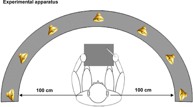
Figure 3. Graphic representation of sound source locations. Seven sound sources were arranged in the participant’s median plane along a frontal arc of ±90° (−90°, −60°, −30°, 0, +30°, +60°, +90°) and centered on the participant’s head (1.0 m distance).

Data Acquisition

Continuous EEG was acquired through the ActiveTwo Biosemi^™ electrode system from 168 scalp electrodes, digitized at 512 Hz. For display purposes, data were filtered with a low-pass 0-phase shift 96 dB 40 Hz filter after acquisition. The reference electrode was assigned in software after acquisition. BioSemi replaces the “ground” electrodes that are used in conventional systems with two separate electrodes: common mode sense (CMS) active electrode and driven right leg (DRL) passive electrode. These two electrodes form a feedback loop, thus rendering them “references.” For a detailed description of the referencing and grounding conventions used by the Biosemi active electrode system, the interested reader is referred to the following website: http://www.biosemi.com/faq/cms&drl.htm. All data were re-referenced to the nasion after acquisition, for analysis (in one subject, the supranasion was used for re-referencing, as the nasion was contaminated by artifact). After each recording session, before the electrode cap was removed from the subject’s head, the 3D coordinates of all 168 electrodes with reference to anatomic landmarks on the head (nasion, pre-auricular notches) were digitized using a Polhemus Magnetic 3D digitizer. EEG was averaged offline. Data were epoched (−100 ms pre-stimulus to 500 ms post-stimulus) and then averaged. Baseline was defined as the mean voltage over −100 to 0 ms preceding the onset of the stimulus. Trials with blinks and large eye-movements were rejected offline on the basis of horizontal and vertical electro-oculogram recordings. An artifact rejection criterion of ±100 μV was used at all other electrode sites to exclude periods of muscle artifact and other noise-transients. From the remaining artifact-free trials, averages were computed for each subject. These averages were then visually inspected for each individual to ensure that clean recordings with sufficient numbers of trials were obtained and that no artifacts were still included. Across both WHAT and WHERE conditions, the average number of accepted sweeps was over 2000 trials. Prior to group averaging, data at electrodes contaminated by artifacts were interpolated for each subject. As described by Greischar et. al 2004, spherical spline interpolation represents a method for increasing power at electrode sites where data has been contaminated. Data were re-baselined over the interval −50 to 20 ms after interpolating. Data were ultimately averaged across all subjects (grand mean averages) for visual comparison at the group level and for display purposes. The reader should note that throughout this paper, we use the familiar nomenclature of the modified 10–20-electrode system to refer to the positioning of electrode sites. Since our montage contains considerably more scalp-sites than this nomenclature allows for, in some cases, we will be referring to the nearest neighboring site within the 10–20 system.

Analysis Strategy

For each electrode, the data for all non-target trials from all subjects were collapsed into a single average waveform for each of the sound sources and averaged over all seven locations. These group-averaged waveforms were then visually inspected across all scalp-sites. To constrain our analyses, we first identified the well-characterized auditory components prior to and including the N1: P20, Pa, P1, and N1. Components were identified on the basis of their expected latencies, over scalp regions previously identified as those areas of maximal amplitude for auditory evoked componentry (see, for example, Picton et al., 1974; Leavitt et al., 2007). Note that the latencies and topographies of the basic AEP components reported here were entirely typical of those previously reported. Analyses were performed across three pairs of scalp electrodes for each component; we chose three electrodes at homologous locations on each side of the scalp (for a total of six electrodes) that best represented the maximal amplitude of the component of interest in a given analysis and averaged across the three electrodes. Statistical analyses were conducted with the SPSS software package (SPSS version 11.5). Limiting our analyses to those electrodes where the components are maximal represents a conservative approach to the analysis of high-density ERP data and raises the likelihood of missed effects (so-called Type II errors) in these rich datasets. Therefore, an exploratory (post hoc) analysis phase was also undertaken (described below under Statistical Cluster Plots).

For each component of interest (P20, Pa, P1, N1), we calculated the area under the waveform for an epoch centered on the peak of the grand mean (the time window used for each epoch was either 10 or 20 ms depending on the width of the respective component’s peak). We then averaged these measures across the three representative electrode sites for each hemisphere. These area measures were then used as the dependent variable. To investigate differences between the AEPs of subjects in the WHAT and WHERE conditions, we tested each identified component with a 2 × 2 analysis of variance (ANOVA). The factors were condition (WHAT versus WHERE) and hemi-scalp (right versus left).

To verify that our object identification task was effective, we compared the average waveform for responses to targets to the same for the standard (i.e., non-target) stimuli. The Nd component (also referred to as the response negativity) has been shown to be elicited when subjects attend to relevant auditory stimuli, when relevance is defined along a physical dimension (Hansen and Hillyard, 1980; Molholm et al., 2004). The presence of a robust Nd component would provide confirmation that our subjects were in fact actively engaged in the object detection task.

It is important to note that our first level of analysis was performed using an average of all seven sound sources, collapsed into a single waveform for each condition. However, the experiment was designed such that every subject was exposed to hundreds of trials from each individual sound source, therefore enabling us to analyze the ERPs generated in response to each spatial location separately. As a second level of analysis, we inspected seven separate waveforms within each condition. We compared these seven averages for our subjects both within and across condition.

Source Reconstruction

Source reconstructions were generated by applying the minimum-norm least squares method as implemented in the BESA software suite (version 5.1; Gräfelfing, Germany). The minimum-norm approach is a commonly used method to estimate a distributed electrical current image in cortex as a function of time (see e.g., Hamalainen and Ilmoniemi, 1994). The source activities of 1426 regional sources are computed. Since the number of sources is much larger than the number of sensors, the inverse problem is highly underspecified and must be stabilized by a mathematical constraint (i.e., the minimum norm). Out of the many current distributions that can account for the recorded sensor data, the solution with the minimum L2 norm, i.e. the minimum total power of the current distribution, is displayed in BESA. To compute the minimum norm here, we utilized an idealized three-shell spherical head model with a radius of 85 mm and assumed scalp and skull thickness of 6 and 7 mm, respectively. The minimum norm was applied to the data across the latency interval 90–130 ms, spanning the N1 timeframe. Baseline period was used to compute mean noise levels. Weightings were applied to the data as follows: (1) weighting at the individual channel level with a noise scale factor of 1.00; (2) depth-weighting such that the lead field of each regional source was scaled with the largest singular value of the singular value decomposition of the source’s lead field; and (3) spatio-temporal weighting using the signal subspace correlation method of Mosher and Leahy (1998) (dimension setting = 6).

Statistical Cluster Plots

As described above, we took a conservative approach to the analysis of the high-density ERP data in order to limit the number of statistical tests performed, with the spatio-temporal properties of the componentry delimiting the tests. Our conservative approach raises the likelihood of missed effects. We therefore performed an exploratory analysis as a means of fully exploring the richness of our data set and as a hypothesis-generating tool for future research. We have devised a simple method for testing the entire data matrix for possible effects, which we term statistical cluster plots (see Molholm et al., 2002; Murray et al., 2002). These cluster plots were derived by calculating point-wise, paired, two-tailed t-tests between the WHAT and WHERE conditions. The results were then arrayed on a single grid, with scalp regions (electrode positions) plotted on the y axis and post-stimulus time plotted on the x axis, thus providing a snapshot overview of significant differences between conditions across scalp regions over time. In the present data treatment, periods of significant difference were only plotted if an alpha criterion of 0.05 was exceeded and then only if this criterion was exceeded for at least five consecutive data points (∼10 ms; see Wetherill and Levitt, 1965; Foxe and Simpson, 2002).

Topographic Modulations

To statistically identify periods of topographic modulation, we calculate the global dissimilarity (GD; Lehmann and Skrandies, 1980, 1984) between WHAT and WHERE responses for each time point of each subject’s data. GD is an index of configuration differences between two electric fields, independent of their strength. This parameter equals the square root of the mean of the squared differences between the potentials measured at each electrode (versus the average reference), each of which is first scaled to unitary strength by dividing by the instantaneous global field power (GFP). GD can range from 0 to 2, where 0 indicates topographic homogeneity and 2 indicates topographic inversion. To derive statistical significance, the observed GD score at each time point was compared against a Monte Carlo distribution composed of 5000 iterations (see Strik et al., 1998 for a description). Statistical significance was determined when the observed GD score (i.e., the mean GD across participants) was ±2 SD away from the mean of the Monte Carlo distribution. Since electric field changes are indicative of changes in the underlying generator configuration (Fender, 1987; Lehmann, 1987, this non-parametric test, in combination with the scalp distributions, provides a reliable measure for determining if and when the brain networks activated by the WHAT and WHERE conditions differ significantly.

Results

Behavioral Results

WHAT condition: group-averaged accuracy across all trials for the sound identification task was 85.4%. WHERE condition: for the sound localization task, 11 participants’ responses were analyzed (one subject’s responses had to be excluded from the behavioral analysis as they were not captured due to a computer malfunction). Each participant’s responses were averaged separately for each of the seven sound source locations; group-averaged responses are displayed in Figure 4. The average offset of responses collapsed over all seven locations was 10.6° ± 12.0°. The average offset to sound source 4, the midline sound source (where we might well expect a very high degree of accuracy) was 4.5°; moreover, all 11 subjects erred to the left of center. Greater accuracy was seen for responses to sound sources located in participants’ left hemifield (Sound sources 1, 2, 3), as compared to right hemifield (Sound sources 5, 6, 7). The average offset for responses to left sound sources (averaging over sound sources 1, 2, and 3) was 3.6° ± 11.0°. Average offset to sound sources in subjects’ right hemifield (averaging over 5, 6, and 7) was 11.7° ± 9.3°. This between hemifield difference was significant (p = 0.006).

FIGURE 4

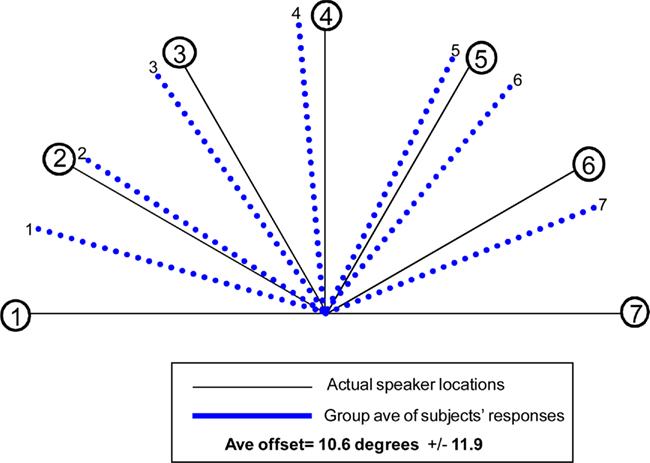
Figure 4. Behavioral results for the “WHERE” condition. Blue lines identify the average of responses across 11 participants (one had to be excluded due to a technical problem capturing responses) for each of the seven sound source locations. Average offset of responses for all seven locations collapsed was 10.6° ± 12°.

Electrophysiological Results I: General Description

In both tasks, stimuli elicited clear ERPs, which contained P20, Pa, P1, and N1 components (Figure 5) with typical scalp distributions (Figure 6). The time period 15–25 ms was selected around the P20 peak in our dataset. An ANOVA revealed no significant main effect of task, WHAT versus WHERE, (F_1,11 = 0.006, p = 0.938), nor was there a significant interaction effect for condition by hemisphere (F_1,11 = 2.509, p = 0.141). The Pa peak in our data was at approximately 42 ms; analysis of 10-ms time window around the peak of the Pa found neither a main effect of condition (F_1,11 = 1.061, p = 0.325), nor for condition by hemisphere (F_1,11 = 0.079, p = 0.783). The P1 peak was found at approximately 62 ms. Analysis of a 10-ms time window around the peak of the P1 yielded neither a main effect of condition (F_1,11 = 0.966, p = 0.347), nor a condition by hemisphere interaction (F_1,11 = 0.298, p = 0.596). In our data, the N1 was evident as a negativity that peaked fronto-centrally at approximately 124 ms in both conditions. To account for the broader deflection of this component, a 20-ms time window was selected around the peak of the N1 (114–134 ms). Here, we found a significant main effect of condition (F_1,11 = 5.811, p = 0.035), reflecting substantially greater amplitude of the N1 in the WHAT condition. The effect size of this difference was 0.64 (using the criteria of Cohen’s d). There was no condition by hemisphere interaction for the N1 component (F_1,11 = 0.455, p = 0.514).

FIGURE 5

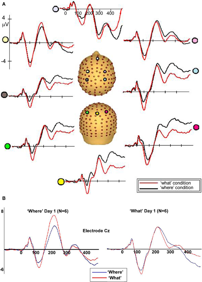
Figure 5. (A) Auditory evoked potentials in participants generated during the WHAT task (red) and the WHERE task (black). Data from eight electrodes spanning frontal, central, and centro-parietal regions are presented. (B) Representative electrode from subgroups of the six subjects who participated in the WHAT condition first (Day 1) and the six who participated in the WHERE condition first.

FIGURE 6

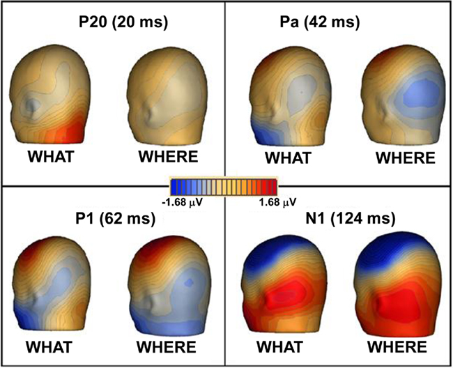
Figure 6. Topographic maps of ERPs recorded during WHAT and WHERE tasks. Group-averaged data are displayed for peak of each auditory component: P20, Pa, P1, and N1.

To rule out the possibility of order effects, subjects who completed the WHERE condition on Day 1 were compared to those who completed the WHAT condition on Day 1 (Figure 5B). As described in the text, the figure demonstrates that both groups (small N of 6 notwithstanding) showed an N1 difference between conditions that is consistent with that shown by the full group, and is detailed in our main results for the full group. Importantly, the direction of the difference is consistent with the full group analysis.

To ensure that subjects’ responses actually reflected attentional processing of relevant auditory stimuli, we compared the response evoked by target stimuli with that of non-target stimuli. As shown in Figure 7, the response elicited by stimuli that included a target auditory element became more negative-going than the responses elicited by the stimuli without a target auditory element over central/fronto-central scalp. This difference extended to about 350 ms. This response pattern is consistent with elicitation of the auditory selective attention component, the Nd (see, for example, Hansen and Hillyard, 1980; Molholm et al., 2004), thereby providing us with compelling evidence that our subjects were truly engaged in a task of sound object recognition.

FIGURE 7

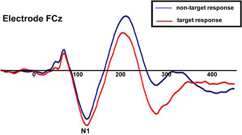
Figure 7. Group-averaged waveforms for responses to the sound object recognition (WHAT) task for target stimuli (red) versus non-target stimuli (blue). Representative electrode shown is FCz.

To better detect missed effects between conditions, we computed a statistical cluster plot for all seven sound sources collapsed into one waveform for each condition (see Materials and Methods). This served as a hypothesis-generating tool; it provided us with a snapshot of where and when significant differences occurred between conditions that may have been missed in our planned analyses. Consistent with our previous analysis, we observed a distinct cluster that coincided with the N1 (Figure 8). What proved to be rather striking was the almost complete absence of any other differences, particularly at later time-points where higher-order cognitive effects generally tend to become evident in ERPs.

FIGURE 8

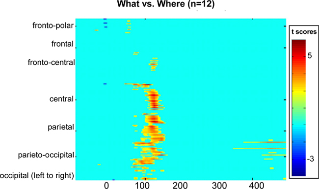
Figure 8. Statistical cluster plot of the results of the point-wise running two-tailed t-tests comparing the amplitudes of participants’ auditory evoked potentials in the WHAT versus WHERE conditions. Time with respect to stimulus onset is presented on the x axis and topographic regions of 168 electrode positions on the y axis. Color corresponds to t values. Periods of significant difference are only plotted if a strict alpha criterion of <0.05 was exceeded for at least five consecutive data points.

A topographic map of the differences between conditions for the N1 timeframe (Figure 9) reveals a topography that is not consistent with auditory components generated in primary auditory cortex. Indeed, it is suggestive of substantial contributions from frontal generators, thereby reflecting processes that more likely involve ventral auditory pathway.

FIGURE 9

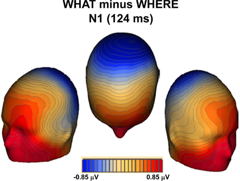
Figure 9. Topographic map of the differences between conditions (WHAT minus WHERE) during the N1 timeframe.

Electrophysiological Results II: Location Specific Averages

We examined each of the seven separate sound source averages within each condition to determine whether evidence of an interaction between sound source location and task could be seen. When we compared between tasks, the N1 difference was consistent; that is, the N1 amplitude in the WHAT task was consistently greater than in the WHERE task (Figure 10A). To determine the significance of this and to probe for any further effects, individual statistical cluster plots for each sound source location were generated. A significant difference between conditions emerged around the time window for the N1 at each sound source location with the exception of Sound source 4 (the midline sound source). It is important to note that the latency of the difference was shifted, depending on the spatial orientation of the sound source. That is, for Sound source 1, the between-condition difference emerged the earliest, prior to 100 ms (∼80 ms), while the difference at Sound source 7 became significant after 100 ms (∼120 ms). A closer inspection of the individual sound source waveforms revealed that the N1 peak was actually later for responses to Sound source 7 than Sound source 1 in both conditions, by approximately 10 ms. This determination was made by a visual inspection of midline electrodes where the N1 was maximal; therefore, the effect cannot be due to laterality effects. For both the WHAT and WHERE tasks, the N1 responses to each individual sound source location from one representative electrode where the N1 component is maximal (Fz) were overlaid and these are presented in Figure 10B. Whereas, in the object task, the N1 response elicited to each sound source was highly stable in that the amplitude was very similar across sound sources, the spatial task evoked responses to each sound source location that showed greater variability. To test this statistically, a 2 × 2 × 7 ANOVA was conducted with factors of condition (WHAT versus WHERE), sound source (1–7), and sound source hemifield (left versus right) to determine whether there was a significant interaction between sound source location and task. We took the average N1 amplitude from three fronto-central electrodes (around FCz) using a 40-ms time window around the N1 peak (importantly, this window was shifted such that it centered on the peak of the N1 for each sound source, as these latencies varied). No significant interaction was found for sound source by condition [F(2,10) = 1.057, p > 0.1], nor was there a three-way interaction between hemifield, sound source, and condition [F(2,10) = 0.410, p > 0.1].

FIGURE 10

Figure 10. (A) WHAT (red) and WHERE (blue) group-averaged waveforms taken from electrode Cz are shown for seven individual sound source averages. In the figure, each waveform pair is shown at a location consistent with the sound source from which it was derived. (B) Separate waveforms for each of the sound sources are overlaid from each condition at one representative electrode (Fz). (C) Topographic maps of the N1 difference between conditions (WHAT minus WHERE) showing distinct topographies for sound sources on the left (Sound sources 1–2–3) compared to the right (Sound sources 5–6–7).

Topographic maps of the difference between conditions (WHAT minus WHERE) were created for an average of the left hemifield sound sources (1–2–3) and the right hemifield sound sources (5–6–7). Subtle but distinct differences can be seen for these, suggesting contributions from unique underlying generator configurations to stimuli that come from the left hemifield compared to those from the right (Figure 10C).

Topographic Modulation Analysis

Averaging across all seven spatial locations, the GD metric allowed us to identify a distinct period of statistically significant differences in topographic modulations between the WHAT and WHERE conditions over the N1 period, indicative of the activation of distinct configurations of intracranial brain generators for each experimental condition (Figure 11). That is, the observed effect at N1 was not only due to a change in the amplitude of activation within a given generator configuration, but crucially, to actual differences in the configurations of neural generators underlying the two tasks (either in the actual neural generators involved, or in the relative contributions from the same set of neural generators).

FIGURE 11

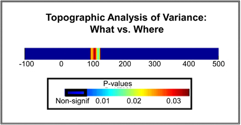
Figure 11. Statistical plot of topographic modulations. Areas of non-significance appear in blue; areas where significance exceeds p < 0.03 are displayed in a graduated color scheme according to the legend shown. Note that this significance cluster falls in a time frame coincident with the N1 component.

Cortical Activation: Minimum-norm Maps

As described in the Methods, the baseline period was used to compute mean noise levels for the source reconstructions, resulting in a signal-to-noise ratio for the selected epoch of 8.67. Source reconstructions at 10 ms intervals, starting from 90 ms, suggested a strong left hemisphere bias for differential processing between conditions (see Figure 12). Two stable clusters of activation, suggestive of separable processing streams, can be seen. At 90 ms, the strongest activation is seen in a cluster over left inferior and superior parietal areas, and this activation continues to be apparent throughout the sampled epoch, although it weakens as time progresses. This cluster is anatomically compatible with the dorsal auditory pathway. The second stable cluster, compatible with the ventral auditory pathway, emerges at approximately 100 ms over anterior temporal regions and peaks at 110 ms, after which point it dissipates substantially. As such, these two activation clusters appear to have some WHAT different time courses. Activation in the right hemisphere suggests much less involvement of underlying generators.

FIGURE 12

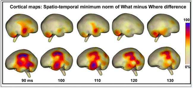
Figure 12. Cortical maps displaying the spatio-temporal minimum-norm topographies for WHAT minus WHERE difference waveforms.

Results for Alternate WHAT Paradigm: WHAT II

Given that only a subset of participants (n = 6) completed the WHAT II paradigm, results should be interpreted cautiously. However, a very specific prediction was being tested here, namely, that a manipulation of the task would not affect the N1 difference seen between the WHAT and WHERE conditions. Behavioral performance accuracy in the WHAT II condition did not differ significantly from WHAT I. A statistical cluster plot analysis comparing the two WHAT paradigms across the entire epoch (−100 to 500) failed to find any areas of significance, suggesting that the differences between WHAT I and WHAT II were negligible (plots not shown). These results support the notion that one paradigm was just as effective as the other in characterizing neural processes underlying sound identification. Next, we conducted an analysis comparing WHAT II and WHERE. We reasoned that if differences between these tasks were found it would support the view that both WHAT I and WHAT II are tapping processes of sound object identification, distinct from processes of sound localization. We used a one-tailed t-test, guided by our hypothesis that the difference between these conditions would replicate the direction seen for WHAT I versus WHERE. The N1 difference was apparent between conditions. Comparing the waveforms, we saw that the direction of the effect was the same: WHAT II resulted in a greater deflection of the N1 relative to WHERE, as seen in WHAT I (Figure 13). While the absolute magnitude of the difference between WHAT II and WHERE is not the same as that of WHAT I versus WHERE, given that the number of subjects in WHAT II was only a subset of the full sample (n = 6), this was likely a power issue and as such, not an unexpected finding.

FIGURE 13

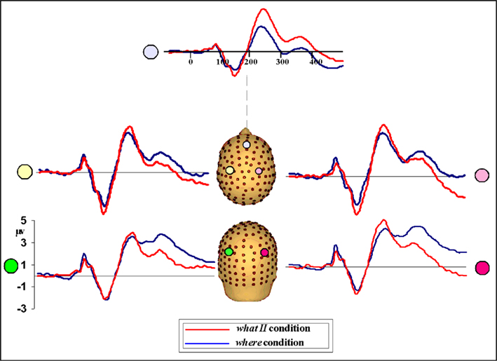
Figure 13. Waveforms from participants (n = 6) comparing performance in WHAT II and WHERE conditions. The direction of the N1 amplitude difference between conditions mirrors that seen in WHAT I versus WHERE; that is, the N1 amplitude for WHAT II is greater than WHERE.

Discussion

The present data showed a robust difference in processing over a surprisingly delimited time frame for subjects performing a task of sound object recognition versus sound localization using exactly the same stimulus setup. This difference was characterized by greater negative-going amplitude during the N1 processing timeframe for the WHAT condition compared to the WHERE condition. This effect was seen consistently at electrode sites over frontal, central, centro-parietal and parietal scalp regions. While this difference occurred during the N1 timeframe, it was clearly not a simple modulation of N1 amplitude as it had a completely different topographic distribution to that of the N1. GD measures using topographic modulation analysis confirmed that the difference between tasks during this timeframe was driven by a shift in the underlying generator configuration. Additionally, applying a minimum-norm source reconstruction algorithm to the difference wave revealed distinct activations that corresponded well with activity within putative dorsal and ventral auditory structures.

The main goal of the present investigation was to find the earliest discernible point of differential processing in the context of spatial and non-spatial auditory tasks. However, a crucial distinction must be made here, and that is that feature processing pathways in cortex are not laid out as one-way highways. Namely, when auditory information is received, it comprises both spatial and non-spatial object features. While the organism may be biased to preferentially process one or the other of these aspects at any given time, this is not to say that the stimulus is stripped of its unattended features. Findings from studies of MMN make clear that both location and object-based properties of auditory stimuli are automatically processed even when attention is directed away from the auditory modality (e.g., Paavilainen et al., 1989; Molholm et al., 2005; Tata and Ward, 2005; Ritter et al., 2006; Näätänen et al., 2007); indeed, MMNs to these features are automatically elicited in people when they are asleep (e.g., Ruby et al., 2008) or even in a coma (e.g., Fischer et al., 2000; Wijnen et al., 2007). Moreover, there is a clear suggestion from our prior investigation of mid-latency auditory evoked responses that there is a constitutive divergence of activation into separable pathways in the context of a passive listening task (Leavitt et al., 2007). While that study was not designed to expressly test the functionality of the dorsal and ventral auditory pathways, automatic sensory activation of these pathways is an inherent result of receiving any auditory stimulation or performing any auditory task. Here, we asked subjects to actively attend to one stimulus feature, location, or identity, in a given condition. Clearly, however, neural processing of the “unattended” feature occurred to some degree as well. There is a growing body of functional imaging literature showing that irrelevant features of objects seem to be processed by the brain, despite having no current task relevance (e.g., O’Craven et al., 1999; Wylie et al., 2004). This strong bias for attention to spread to non-primary stimulus features has also been shown cross-modally, using audio-visual tasks (Molholm et al., 2004, 2007; Fiebelkorn et al., 2010a, b). This spread of attention is further evidenced by findings in the visual modality that directing spatial attention to one part of an object results in the facilitation of sensory processing across the entire extent of that object (e.g., Egly et al., 1994; Martinez et al., 2007). Therefore, while in the present investigation we have identified a point of task-specific divergence at approximately 120 ms, it is extremely unlikely that this represents the first point at which processing for these qualities truly begins.

Two previous studies of object versus spatial processing have also shown amplitude modulation during the auditory N1 timeframe, but in both of these, the direction of the effect was actually opposite to that seen here, with responses in the WHERE condition showing larger amplitude (Ahveninen et al., 2006; De Santis et al., 2007a). A third MEG study found no amplitude differences for N1 (Anourova et al., 2001), but rather, a latency difference between tasks. These differences are likely explained by paradigmatic differences. The stimuli used by these investigators were simple tones (Anourova et al., 2001; De Santis et al., 2007a) and vowel pairs (Ahveninen et al., 2006) and it could be argued that these stimuli might be relatively less effective at activating object-processing regions. Here, by employing complex, and considerably more ecological sounds, it is likely that greater activation of WHAT processing regions was invoked. Whereas sound localization may be more automatic, and engaged more quickly (as suggested by Anourova et al., 2001), object recognition and identification relies more heavily on accessing a memory trace and it is a reasonable assumption that invoking a memory trace of a complex sound such as the animal calls used here, would employ a greater neural network than that of a simple tone. Similarly, in all of these prior investigations, only a limited number of spatial locations were used during the spatial condition. In most, only two positions were used, and in only one case were three used (Anurova et al., 2003). Here, seven discrete locations were used, and therefore performing the current task would have required a great deal more effort, and consequently, greater involvement of underlying neural networks for spatial discrimination. Moreover, our subjects were not explicitly aware that there were seven discrete sound sources, and so the number of sound sources was unknown to them and likely created higher demands on them relative to past studies utilizing less sound sources. In sum, we suggest that the paradigm employed in the current study was both: (1) more challenging in both the WHAT and WHERE conditions than prior studies employing less complex, and fewer stimulus types, and (2) more ecologically valid, and therefore provided results which more accurately reflect the way we actually process auditory information in the complex world around us.

It could be considered surprising that while we found significant task-related differences during the N1 processing timeframe, there were no subsequent time-points where significant differences were seen. With such different tasks as localizing sound and making a sound object identification, one might well predict that distinct higher-order cognitive processes might be engaged at later latencies, such as the P300 component, which has been shown to index attention-related information processing (e.g., Polich, 1986; Linden, 2005). On the other hand, the lack of differences during later timeframes here provides good confirmation that higher-order attentional processes were not differentially engaged between the two tasks, suggesting that the location and recognition tasks were well-matched for difficulty. This suggestion, however, must be considered in the context of our notion that the use of animal calls in the present study is what made our design both more ecologically valid, and more accurate in identifying a greater allocation of neural resources as evidenced exclusively by the higher amplitude N1 component seen in the WHAT condition. Whether such a focal deployment of attentional resources (that is, limited only to the N1 period) can be measured in an experimental paradigm engaging sensory modalities other than the auditory system remains to be investigated by future studies.

The behavioral findings for the WHERE task are noteworthy, in that they appear to represent an auditory analog to the pattern of pseudoneglect that has been consistently observed in the visual system of healthy controls. Specifically, pseudoneglect refers to a leftward attentional bias that occurs in normally functioning individuals and causes them to bisect visually presented lines slightly to the left of their true center (e.g., McCourt, 2001; Foxe et al., 2003; McCourt et al., 2008). This spatial bias has been attributed to the well-known right hemisphere specialization for spatial attention (see e.g., Mesulam, 2000), and indeed, both functional imaging (Fink et al., 2001 and ERP studies (Foxe et al., 2003) show that visuospatial judgments during line-bisection are subserved by right parietal regions. Here, subjects consistently mislocated the centrally presented sound approximately 4.5° leftward of veridical center. This leftward bias can also be seen for the pair of closest flanking sound sources (sound sources 3 and 5). Another interesting aspect of these data was the observation of significantly more accurate responses to the three sound sources in the left hemisphere (Sound sources 1, 2, 3) than to the three sound sources in the right hemisphere (Sound sources 5, 6, 7). This is consistent with what is known about hemispheric differences in sound localization in humans; namely, that auditory spatial processing is more accurate for sounds in the left hemifield (Burke et al., 1994), again presumably because of the right hemisphere bias for spatial attention. Indeed, these investigators interpreted their findings to suggest a pivotal role for right hemisphere in auditory spatial acuity. In agreement, other studies have implicated greater involvement of the right hemisphere in sound localization (see e.g., Farah et al., 1989; Hausmann et al., 2005; Tiitinen et al., 2006; Mathiak et al., 2007).

It is of note that we did not find specific lateralization of the main effect reported here between the WHAT and WHERE tasks, with no evidence for a hemisphere by condition interaction in our main ERP analysis. However, the ensuing source-localization did suggest that there may in fact be a left hemisphere bias, which would be in accord with literature providing evidence for a left lateralization effect of the WHERE pathway during speech sound processing (Mathiak et al., 2007), as well as evidence for involvement of language-dominant inferior dorsolateral frontal lobe in processing non-verbal auditory information (Mathiak et al., 2004). It will fall to future work to specifically test whether there is hemispheric specialization for processing of WHAT and WHERE auditory stimuli.

Human lesion studies

Human lesion studies provide additional support for the division of the auditory system into dorsal and ventral pathways (Clarke et al., 2000, 2002; Clarke and Thiran, 2004). In a series of case studies, Clarke et al. (2000) investigated auditory recognition and localization in four patients with circumscribed left hemisphere lesions. Two of four patients showed impaired recognition of environmental sounds but intact ability to localize sounds. In one, the lesion included postero-inferior portions of the frontal convexity and the anterior third of the temporal lobe. In the other, the lesion included left superior, middle and inferior temporal gyri, and lateral auditory areas, but spared Heschl’s gyrus, the acoustic radiation, and the thalamus. The third patient was impaired in auditory motion perception and localization, but had preserved environmental sound recognition; here, the lesion included the parieto-frontal convexity and the supratemporal region. The fourth patient was impaired in both tasks, with a lesion comprising large portions of the supratemporal region, temporal, postero-inferior frontal, and antero-inferior parietal convexities. A subsequent investigation by the same group examined 15 patients with right focal hemispheric lesions (Clarke et al., 2002). Again, sound recognition and sound localization were shown to be disrupted independently. In this study, patients with selective sound localization deficits tended to have lesions involving inferior parietal and frontal cortices, as well as superior temporal gyrus, whereas patients with selective recognition deficits had lesions of the temporal pole, the anterior part of fusiform, and the inferior and middle temporal gyrus. This double dissociation clearly supports somewhat independent processing streams for sound recognition and sound localization in humans.

Conclusion

In this study, we asked participants to make judgments about the spatial location of sounds versus the object-identity of those same sounds, with an eye to assessing whether varying task set in this manner would engage dissociable neural circuits within auditory cortices. These tasks were chosen to tap so-called WHERE and WHAT processes, which have been associated with dorsal and ventral regions of the auditory system respectively. Our high-density electrical mapping data revealed a robust difference in the ERP during the timeframe of the auditory N1 component and topographic analysis pointed to differential engagement of underlying auditory cortices during this timeframe. Source-analysis supported the main thesis in that this differential processing was generated in dissociable regions of the dorsal and ventral auditory processing stream.

Acknowledgments

Support for this work was provided by a grant from the US National Institute of Mental Health (RO1-MH65350 to John J. Foxe; RO1-MH85322 to Sophie Molholm and John J. Foxe) and by a Ruth L. Kirschstein pre-doctoral fellowship to Victoria M. Leavitt (NRSA – MH74284). The authors thank Daniella Blanco, Megan Perrin, and Jennifer Montesi for their invaluable assistance with data collection.

References

Ahveninen, J., Jaaskelainen, I. P., Raij, T., Bonmassar, G., Devore, S., Hamalainen, M., Levanen, S., Lin, F. H., Sams, M., Shinn-Cunningham, B. G., Witzel, T., and Belliveau, J. W. (2006). Task-modulated “what” and “where” pathways in human auditory cortex. Proc. Natl. Acad. Sci. U.S.A. 103, 14608–14613.

CrossRef Full Text

Alain, C., Arnott, S. R., Hevenor, S., Graham, S., and Grady, C. L. (2001). “WHAT” and “where” in the human auditory system. Proc. Natl. Acad. Sci. U.S.A. 98, 12301–12306.

CrossRef Full Text

Anourova, I., Nikouline, V. V., Ilmoniemi, R. J., Hotta, J., Aronen, H. J., and Carlson, S. (2001). Evidence for dissociation of spatial and nonspatial auditory information processing. Neuroimage 14, 1268–1277.

CrossRef Full Text

Anurova, I., Artchakov, D., Korvenoja, A., Ilmoniemi, R. J., Aronen, H. J., and Carlson, S. (2003). Differences between auditory evoked responses recorded during spatial and nonspatial working memory tasks. Neuroimage 20, 1181–1192.

CrossRef Full Text

Arnott, S. R., Binns, M. A., Grady, C. L., and Alain, C. (2004). Assessing the auditory dual-pathway model in humans. Neuroimage 22, 401–408.

CrossRef Full Text

Belin, P., and Zatorre, R. J. (2000). “WHAT”, “where” and “how” in auditory cortex. Nat. Neurosci. 3, 965–966.

CrossRef Full Text

Burke, K. A., Letsos, A., and Butler, R. A. (1994). Asymmetric performances in binaural localization of sound in space. Neuropsychologia 32, 1409–1417.

CrossRef Full Text

Clarke, S., Bellmann, A., Meuli, R. A., Assal, G., and Steck, A. J. (2000). Auditory agnosia and auditory spatial deficits following left hemispheric lesions: evidence for distinct processing pathways. Neuropsychologia 38, 797–807.

CrossRef Full Text

Clarke, S., Bellmann Thiran, A., Maeder, P., Adriani, M., Vernet, O., Regli, L., Cuisenaire, O., and Thiran, J. P. (2002). WHAT and where in human audition: selective deficits following focal hemispheric lesions. Exp. Brain Res. 147, 8–15.

CrossRef Full Text

Clarke, S., and Thiran, A. B. (2004). Auditory neglect: WHAT and where in auditory space. Cortex 40, 291–300.

CrossRef Full Text

De Santis, L., Clarke, S., and Murray, M. M. (2007a). Automatic and intrinsic auditory “WHAT” and “where” processing in humans revealed by electrical neuroimaging. Cereb. Cortex 17, 9–17.

CrossRef Full Text

De Santis, L., Spierer, L., Clarke, S., and Murray, M. M. (2007b). Getting in touch: segregated somatosensory WHAT and where pathways in humans revealed by electrical neuroimaging. Neuroimage 37, 890–903.

CrossRef Full Text

Egly, R., Driver, J., and Rafal, R. D. (1994). Shifting visual attention between objects and locations: evidence from normal and parietal lesion subjects. J. Exp. Psychol. Gen. 123, 161–177.

CrossRef Full Text

Fabiani, M., Kazmerski, V. A., Cycowicz, Y. M., and Friedman, D. (1996). Naming norms for brief environmental sounds: effects of age and dementia. Psychophysiology 33, 462–475.

CrossRef Full Text

Farah, M. J., Wong, A. B., Monheit, M. A., and Morrow, L. A. (1989). Parietal lobe mechanisms of spatial attention: modality-specific or supramodal? Neuropsychologia 27, 461–470.

CrossRef Full Text

Fender, D. H. (1987). “Source localization of brain electrical activity,” in Handbook of Electroencephalography and Clinical Neurophysiology, Revised Series, Vol. 1: Methods of Analysis of Brain Electrical and Magnetic Signals, eds A. S. Gevins and A. Remond (Amsterdam: Elsevier), 355–399.

Fiebelkorn, I. C., Foxe, J. J., Schwartz, T. H., and Molholm, S. (2010a). Staying within the lines: the formation of visuospatial boundaries influences multisensory feature integration. Eur. J. Neurosci. 31, 1737–1743.

CrossRef Full Text

Fiebelkorn, I. C., Foxe, J. J., and Molholm, S. (2010b). Dual mechanisms for the cross-sensory spread of attention: how much do learned assocations matter? Cereb. Cortex 20, 109–120.

CrossRef Full Text

Fink, G. R., Marshall, J. C., Weiss, P. H., and Zilles, K. (2001). The neural basis of vertical and horizontal line bisection judgments: an fMRI study of normal volunteers. Neuroimage 14(1 Pt 2), S59–S67.

Fischer, C., Morlet, D., and Giard, M. (2000). Mismatch negativity and N100 in comatose patients. Audiol. Neurootol. 5, 192–197.

CrossRef Full Text

Foxe, J. J., McCourt, M. E., and Javitt, D. C. (2003). Right hemisphere control of visuospatial attention: line-bisection judgments evaluated with high-density electrical mapping and source analysis. Neuroimage 19, 710–726.

CrossRef Full Text

Foxe, J. J., and Simpson, G. V. (2002). Flow of activation from V1 to frontal cortex in humans. A framework for defining “early” visual processing. Exp. Brain Res. 142, 139–150.

Greischar, L. L., Burghy, C. A., van Reekum, C. M., Jackson, D. C., Pizzagalli, D. A., Mueller, C., and Davidson, R. J. (2004). Effects of electrode density and electrolyte spreading in dense array electroencephalographic recording. Clin. Neurophysiol. 115, 710–720.

CrossRef Full Text

Hamalainen, M. S., and Ilmoniemi, R. J. (1994). Interpreting magnetic fields of the brain: minimum norm estimates. Med. Biol. Eng. Comput. 32, 35–42.

CrossRef Full Text

Hansen, J. C., and Hillyard, S. A. (1980). Endogenous brain potentials associated with selective auditory attention. Electroencephalogr. Clin. Neurophysiol. 49, 277–290.

CrossRef Full Text

Hausmann, M., Corballis, M. C., Fabri, M., Paggi, A., and Lewald, J. (2005). Sound lateralization in subjects with callosotomy, callosal agenesis, or hemispherectomy. Brain Res. Cogn. Brain Res. 25, 537–546.

CrossRef Full Text

Kaas, J. H., and Hackett, T. A. (1999). “WHAT” and “where” processing in auditory cortex. Nat. Neurosci. 2, 1045–1047.

CrossRef Full Text

Lalor, E. C., Yeap, S., Reilly, R. B., Pearlmutter, B. A., and Foxe, J. J. (2008). Dissecting the cellular contributions to early visual sensory processing deficits in schizophrenia using the VESPA evoked response. Schizophr. Res. 98, 256–264.

CrossRef Full Text

Leavitt, V. M., Molholm, S., Ritter, W., Shpaner, M., and Foxe, J. J. (2007). Auditory processing in schizophrenia during the middle latency period (10–50 ms): high-density electrical mapping and source analysis reveal subcortical antecedents to early cortical deficits. J. Psychiatry Neurosci. 32, 339–353.

Lehmann, D., and Skrandies, W. (1980). Reference-free identification of components of checkerboard-evoked multichannel potential fields. Electroencephalogr. Clin. Neurophysiol. 48, 609–621.

CrossRef Full Text

Lehmann, D., and Skrandies, W. (1984). Spatial analysis of evoked potentials in man – a review. Prog. Neurobiol. 23, 227–250.

CrossRef Full Text

Lehmann, D. (1987). “Principles of spatial analysis,” in Methods of Analysis of Brain Electrical and Magnetic Signals, Handbook of Electroencephalography and Clinical Neurophysiology, Revised Series, Vol. 1, eds. A. S. Gevins and A. Remond (Amsterdam: Elsevier), 309–354.

Linden, D. E. (2005). The p300: where in the brain is it produced and WHAT does it tell us? Neuroscientist 11, 563–576.

Pubmed Abstract | Pubmed Full Text | CrossRef Full Text

Martinez, A., Ramanathan, D. S., Foxe, J. J., Javitt, D. C., and Hillyard, S. A. (2007). The role of spatial attention in the selection of real and illusory objects. J. Neurosci. 27, 7963–7973.

CrossRef Full Text

Mathiak, K., Hertrich, I., Grodd, W., and Ackermann, H. (2004). Discrimination of temporal information at the cerebellum: functional magnetic resonance imaging of nonverbal auditory memory. Neuroimage 21, 154–162.

CrossRef Full Text

Mathiak, K., Menning, H., Hertrich, I., Mathiak, K. A., Zvyagintsev, M., and Ackermann, H. (2007). Who is telling what from where? A functional magnetic resonance imaging study. Neuroreport 18, 405–409.

CrossRef Full Text

McCourt, M. E. (2001). Performance consistency of normal observers in forced-choice tachistoscopic visual line bisection. Neuropsychologia 39, 1065–1076.

CrossRef Full Text

McCourt, M. E., Shpaner, M., Javitt, D. C., and Foxe, J. J. (2008). Hemispheric asymmetry and callosal integration of visuospatial attention in schizophrenia: a tachistoscopic line bisection study. Schizophr. Res. 102, 189–196.

CrossRef Full Text

Mesulam, M. M. (2000). “Attentional networks, confusional states, and neglect syndromes,” in Principles of Behavioral and Cognitive Neurology, ed. M. M. Mesulam (Oxford: Oxford University Press), 174–256.

Mishkin, M., Lewis, M. E., and Ungerleider, L. G. (1982). Equivalence of parieto-preoccipital subareas for visuospatial ability in monkeys. Behav. Brain Res. 6, 41–55.

CrossRef Full Text

Molholm, S., Martinez, A., Ritter, W., Javitt, D. C., and Foxe, J. J. (2005). The neural circuitry of pre-attentive auditory change-detection: an fMRI study of pitch and duration mismatch negativity generators. Cereb. Cortex 15, 545–551.

CrossRef Full Text

Molholm, S., Martinez, A., Shpaner, M., and Foxe, J. J. (2007). Object-based attention is multisensory: co-activation of an object’s representations in ignored sensory modalities. Eur. J. Neurosci. 26, 499–509.

CrossRef Full Text

Molholm, S., Ritter, W., Javitt, D. C., and Foxe, J. J. (2004). Multisensory visual-auditory object recognition in humans: a high-density electrical mapping study. Cereb. Cortex 14, 452–465.

CrossRef Full Text

Molholm, S., Ritter, W., Murray, M. M., Javitt, D. C., Schroeder, C. E., and Foxe, J. J. (2002). Multisensory auditory-visual interactions during early sensory processing in humans: a high-density electrical mapping study. Brain Res. Cogn. Brain Res. 14, 115–128.

CrossRef Full Text

Mosher, J. C., and Leahy, R. M. (1998). Recursive MUSIC: a framework for EEG and MEG source localization. IEEE Trans. Biomed. Eng. 45, 1342–1354.

CrossRef Full Text

Murray, M. M., Wylie, G. R., Higgins, B. A., Javitt, D. C., Schroeder, C. E., and Foxe, J. J. (2002). The spatiotemporal dynamics of illusory contour processing: combined high-density electrical mapping, source analysis, and functional magnetic resonance imaging. J. Neurosci. 22, 5055–5073.

Näätänen, R., Paavilainen, P., Rinne, T., and Alho, K. (2007). The mismatch negativity (MMN) in basic research of central auditory processing: a review. Clin. Neurophysiol. 118, 2544–2590.

CrossRef Full Text

Nousak, J. M., Deacon, D., Ritter, W., and Vaughan, H. G. Jr. (1996). Storage of information in transient auditory memory. Brain Res. Cogn. Brain Res. 4, 305–317.

CrossRef Full Text

O’Craven, K. M., Downing, P. E., and Kanwisher, N. (1999). fMRI evidence for objects as the units of attentional selection. Nature 401, 584–587.

CrossRef Full Text

Oldfield, R. C. (1971). The assessment and analysis of handedness: the Edinburgh inventory. Neuropsychologia 9, 97–113.

CrossRef Full Text

Paavilainen, P., Karlsson, M. L., Reinikainen, K., and Näätänen, R. (1989). Mismatch negativity to change in spatial location of an auditory stimulus. Electroencephalogr. Clin. Neurophysiol. 73, 129–141.

CrossRef Full Text

Picton, T. W., Hillyard, S. A., Krausz, H. I., and Galambos, R. (1974). Human auditory evoked potentials. I. Evaluation of components. Electroencephalogr. Clin. Neurophysiol. 36, 179–190.

CrossRef Full Text

Polich, J. (1986). Attention, probability, and task demands as determinants of P300 latency from auditory stimuli. Electroencephalogr. Clin. Neurophysiol. 63, 251–259.

CrossRef Full Text

Poremba, A., Saunders, R. C., Crane, A. M., Cook, M., Sokoloff, L., and Mishkin, M. (2003). Functional mapping of the primate auditory system. Science 299, 568–572.

CrossRef Full Text

Rämä, P., Poremba, A., Sala, J. B., Yee, L., Malloy, M., Mishkin, M., and Courtney, S. M. (2004). Dissociable functional cortical topographies for working memory maintenance of voice identity and location. Cereb. Cortex 14, 768–780.

CrossRef Full Text

Rauschecker, J. P., and Tian, B. (2000). Mechanisms and streams for processing of “what” and “where” in auditory cortex. Proc. Natl. Acad. Sci. U.S.A. 97, 11800–11806.

CrossRef Full Text

Ritter, W., De Sanctis, P., Molholm, S., Javitt, D. C., and Foxe, J. J. (2006). Preattentively grouped tones do not elicit MMN with respect to each other. Psychophysiology 43, 423–430.

CrossRef Full Text

Roeber, U., Widmann, A., and Schroger, E. (2003). Auditory distraction by duration and location deviants: a behavioral and event-related potential study. Brain Res. Cogn. Brain Res. 17, 347–357.

CrossRef Full Text

Romanski, L. M., Tian, B., Fritz, J., Mishkin, M., Goldman-Rakic, P. S., and Rauschecker, J. P. (1999). Dual streams of auditory afferents target multiple domains in the primate prefrontal cortex. Nat. Neurosci. 2, 1131–1136.

CrossRef Full Text

Ruby, P., Caclin, A., Boulet, S., Delpuech, C., and Morlet, D. (2008). Odd sound processing in the sleeping brain. J. Cogn. Neurosci. 20, 296–311.

CrossRef Full Text

Schmolesky, M. T., Wang, Y., Hanes, D. P., Thompson, K. G., Leutgeb, S., Schall, J. D., and Leventhal, A. G. (1998). Signal timing across the macaque visual system. J. Neurophysiol. 79, 3272–3278.

Schroeder, C. E., Mehta, A. D., and Givre, S. J. (1998). A spatiotemporal profile of visual system activation revealed by current source density analysis in the awake macaque. Cereb. Cortex 8, 575–592.

CrossRef Full Text

Strik, W. K., Fallgatter, A. J., Brandeis, D., and Pascual-Marqui, R. D. (1998). Three-dimensional tomography of event-related potentials during response inhibition: evidence for phasic frontal lobe activation. Electroencephalogr. Clin. Neurophysiol. 108, 406–413.

CrossRef Full Text

Tata, M. S., and Ward, L. M. (2005). Early phase of spatial mismatch negativity is localized to a posterior “where” auditory pathway. Exp. Brain Res. 167, 481–486.

CrossRef Full Text

Tian, B., Reser, D., Durham, A., Kustov, A., and Rauschecker, J. P. (2001). Functional specialization in rhesus monkey auditory cortex. Science 292, 290–293.

CrossRef Full Text

Tiitinen, H., Salminen, N. H., Palomaki, K. J., Makinen, V. T., Alku, P., and May, P. J. (2006). Neuromagnetic recordings reveal the temporal dynamics of auditory spatial processing in the human cortex. Neurosci. Lett. 396,17–22.

CrossRef Full Text

Weeks, R. A., Aziz-Sultan, A., Bushara, K. O., Tian, B., Wessinger, C. M., Dang, N., Rauschecker, J. P., and Hallett, M. (1999). A PET study of human auditory spatial processing. Neurosci. Lett. 262, 155–158.

CrossRef Full Text

Wetherill, G. B., and Levitt, H. (1965). Sequential estimation of points on a psychometric function. Br. J. Math. Stat. Psychol. 18, 1–10.

Wijnen, V. J., van Boxtel, G. J., Eilander, H. J., and de Gelder, B. (2007). Mismatch negativity predicts recovery from the vegetative state. Clin. Neurophysiol. 118, 597–605.

CrossRef Full Text

Wylie, G. R., Javitt, D. C., and Foxe, J. J. (2004). Don’t think of a white bear: an fMRI investigation of the effects of sequential instructional sets on cortical activity in a task-switching paradigm. Hum. Brain Mapp. 21, 279–297.

CrossRef Full Text

Zatorre, R. J., Bouffard, M., Ahad, P., and Belin, P. (2002). Where is “where” in the human auditory cortex? Nat. Neurosci. 5, 905–909.

CrossRef Full Text