The interplay of plasticity and adaptation in neural circuits: a generative model

1. Introduction

The main goal of Computational Neuroscience is to uncover the kinds of computation implemented by neurons and neural circuits, and to identify the biological mechanisms underlying these computations. Numerous types of computation have been described and have been associated with the dynamics of different neural and synaptic processes (Herz et al., 2006; Abbott, 2008; Gerstner et al., 2012; Tetzlaff et al., 2012). Among the numerous biological phenomena observed in the brain, sensory adaptation and synaptic plasticity stand out as two of the most studied, since they are observed ubiquitously across most brain regions and animal species. Both phenomena give rise to specific types of computation, but the functional implications of their interaction remain unclear.

Synaptic plasticity is the change in strength of the interaction between neurons, and is believed to control the change in behavior of a subject following its experience of the external world. Synaptic plasticity takes multiple forms (Abbott and Nelson, 2000; Feldman, 2009), of which the most studied is Hebbian plasticity (Bi and Poo, 2001; Caporale and Dan, 2008). Different types of plasticity are believed to underlie a broad range of functions, including: memory formation and storage (Martin et al., 2000; Lamprecht and LeDoux, 2004; Seung, 2009), nervous system development (Katz and Shatz, 1996; Miller, 1996; Sanes and Lichtman, 1999; Song and Abbott, 2001), recovery after brain injury (Buonomano and Merzenich, 1998; Feldman and Brecht, 2005), classical conditioning (Wickens et al., 2003; Calabresi et al., 2007; Surmeier et al., 2009; Pawlak et al., 2010; Gallistel and Matzel, 2013), operant conditioning (Seung, 2003; Montague et al., 2004; Daw and Doya, 2006; Doya, 2007; Soltani and Wang, 2008), spatial navigation (Blum and Abbott, 1996; Mehta et al., 2002), efficient coding of sensory stimuli (Toyoizumi et al., 2005; Savin et al., 2010; Bernacchia and Wang, 2013), homeostatic regulation of neuronal excitability (Royer and Paré, 2003; Turrigiano and Nelson, 2004; Williams et al., 2013), sound localization (Gerstner et al., 1996) and production of behavioral sequences (Fiete et al., 2010).

Sensory adaptation is the change in responsiveness of a neuron to a given input, and is believed to control the change in perception of a stimulus, even if the stimulus maintains constant physical attributes (Webster, 2011). The main effect of adaptation on neural activity is to shift the response function depending on the adapting stimulus (Kohn, 2007; Rieke and Rudd, 2009). This effect has been observed in a broad range of species, sensory modalities and stimulus variables, including: luminance (Sakmann and Creutzfeldt, 1969; Shapley and Enroth-Cugell, 1984), contrast (Ohzawa et al., 1985; Smirnakis et al., 1997), edge orientation (Müller et al., 1999; Dragoi et al., 2000), direction of motion (Kohn and Movshon, 2004), motion speed (Brenner et al., 2000; Krekelberg et al., 2006) and sound level (Dean et al., 2005). In addition to the shift in tuning, the gain of neural response changes depending on the stimulus variance (Fairhall et al., 2001; Borst et al., 2005; Nagel and Doupe, 2006; Maravall et al., 2007). One hypothesized function of sensory adaptation is the efficiency of coding: the statistics of input stimuli can vary widely and must be encoded by neurons with limited dynamic range; centering the neural response around the mean input prevents saturation and determines optimal discrimination (Laughlin, 1981; Wainwright, 1999; Machens et al., 2005; Clifford et al., 2007; Schwartz et al., 2007; Wark et al., 2007).

I simulate and analyze a computational model of a recurrent neural circuit, and I show that when both sensory adaptation and synaptic plasticity are included in the model, the neural circuit is endowed with a specific type of computation: it becomes a generative model of the input stimuli. Generative models provide a solution to a broad range of problems in machine learning (Hinton, 2007, 2010; Barra et al., 2012), and have been proposed as candidate models of perception, learning and Bayesian inference in real brains (Fiser et al., 2010; Clark, 2013). In the model presented here, the spontaneous dynamics of neural activity lingers on a subset of specific neural patterns which correspond to the neural patterns that have been driven by sensory stimuli. In particular, the likelihood of observing a given neural pattern is equal to the frequency with which the corresponding stimulus has been previously experienced. Formally speaking, the model dynamics displays a large number of attractors which sample exactly the probability distribution of input stimuli. In the limit of an infinite number of neurons, I show that the dynamics converges to a continuous (line) attractor.

Neurons and synapses are modeled as binary variables (Hopfield, 1982; Tsodyks, 1990), therefore the model is not biologically realistic. In particular, it does not include separate populations of excitatory and inhibitory neurons and does not account for a range of dynamical regimes observed in the brain, such as the asynchronous and irregular spiking activity of cortical neurons. Also, the network operates in two distinct phases: (1) a stimulus driven regime in which plasticity and adaptation occur and internal dynamics is turned off, and (2) a spontaneous regime in which the stable states of the dynamics are probed in absence of stimulus, plasticity and adaptation. However, the model is very simple to simulate and analyze despite the inclusion of multiple mechanisms. The present work is limited to univariate distributions of input stimuli.

2. Materials and Methods

The neural circuit implemented in this work is a variant of a model studied in Bernacchia and Amit (2007), with the additional inclusion of adaptation. I consider a neural circuit with a total number of neurons equal to N, labeled by the index i = 1, …, N. The total current afferent to neuron i at time t is the sum of the external current, due to the input stimulus, and the internal current, due to the local recurrent connections within the neural circuit:

$\begin{array}{cc}{I}_i(t)=I_i^{ext}(t)+I_i^{int}(t)& (1)\end{array}$

The activity of neuron i upon receiving current I_i is equal to

$\begin{array}{cc}{x}_i(t+\Delta t)=\text{sign}\left(I_i(t)\right)& (2)\end{array}$

where Δt is the time step used in simulations.

For simplicity, I consider two exclusive scenarios, in which either of the two types of currents dominate: When a stimulus is presented, the internal current is set to zero, therefore the external current dominates (“stimulus-driven” stage); when a stimulus is absent, the external current is set to zero and the internal current dominates (“spontaneous” stage). The case in which both types of current are simultaneously contributing was studied in Bernacchia and Amit (2007) (in absence of adaptation). The parameter Δt reflects the time constant of the update of a neuron's activity, and is set to 10 ms during the spontaneous stage. During the stimulus-driven stage, a sequence of stimuli is presented, the activity is instantaneously enforced by the stimulus. Therefore, the activity is constant as long as the stimulus is constant, and changes immediately following transitions between subsequent stimuli. For simplicity, I simulate one time step for each stimulus, by setting the time step equal to one “trial,” Δt = 1. This value of Δt is used only for convenience of numerical integration, and is not related to any biological timescale. A total of T number of trials is simulated (a sequence of T stimuli) in one simulation, t = 1, …, T.

The stimulus identity is labeled by α, varying in the closed interval of real numbers α ∈ (0,1), and the stimulus presented at time t is denoted as α(t). The stimulus value α(t) at each time step is drawn at random from a probability distribution P(α). The external current afferent to neuron i depends on how that neuron is tuned to the stimulus, which is summarized by its “tuning curve.” I consider two types of tuning curves in different simulations, one monotonic (sigmoidal), and one periodic (sine), given by the following simple formulas

$\begin{array}{cc}{I}_i^{ext}(t)=\tanh (\beta [\alpha (t)-{\mu }_i])& (3)\end{array}$

$\begin{array}{cc}{I}_i^{ext}(t)=\sin (2\pi [\alpha (t)-{\mu }_i])& (4)\end{array}$

An illustration of the tuning curves is presented in Figure 1. I define μ_i as the “tuning offset”: different neurons have different offsets, but the same shape of the tuning curve. The results of most simulation are shown for the sigmoidal tuning curve (3), but very similar results have been obtained for a periodic tuning curve (4) (see Appendix). The parameter β is positive, and its specific value is irrelevant, since the neuron output is binary, given by Equation (2), and the internal current is zero during the stimulus. In a given simulation, the probability distribution P(α) is taken from a parametric family (see e.g., Figure 3), and different parameters are drawn at random in different simulations (the distribution equals the square of a Fourier series with random coefficients truncated at five terms).

FIGURE 1

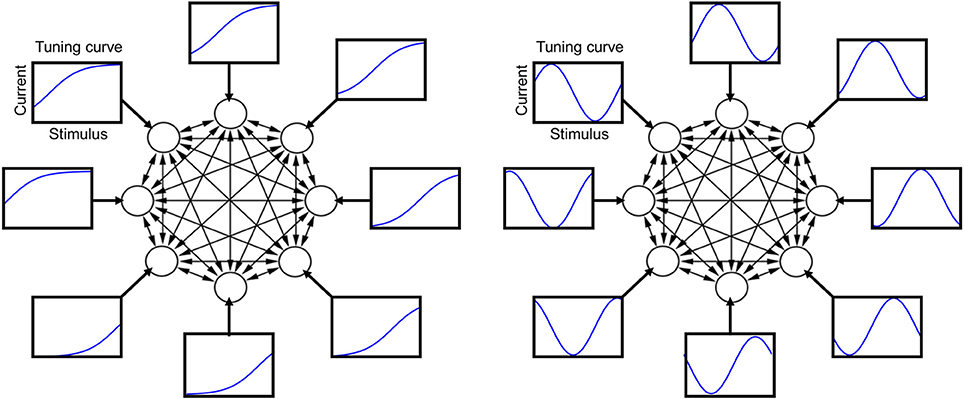
Figure 1. Schematic illustration of the neural circuit model with its tuning curves and recurrent connections. Each circle represents one neuron and each arrow a synaptic connection. Each rectangle shows a tuning curve for one neuron, namely the external current afferent to that neuron plotted as a function of the stimulus value. Left: sigmoidal tuning curves. Right: periodic tuning curves.

The internal current is the sum of activity x_j of pre-synaptic neurons weighted by the synaptic matrix J_ij, namely

$\begin{array}{cc}{I}_i^{int}(t)=\frac{1}{2N}{\displaystyle \sum _j{J}_{ij}}(t)x_j(t)& (5)\end{array}$

Synaptic weights have binary values, J_ij = ±1, except for the self-couplings that are set to zero J_ii = 0. Synaptic strengths are initialized at random, +1 and −1 with equal probability. The synaptic plasticity rule is Hebbian, meaning that it follows the correlation of the pre and post-synaptic neuron (the product x_ix_j). Synaptic weights are updated at random at each time step according to the following transition probabilities. The probability of potentiation from time t to time t + Δt is the probability of the transition from J_ij(t) = −1 to J_ij(t + Δt) = +1, and is defined as

$\begin{array}{cc}{w}_{+}=\frac{1+x_i{x}_j}{2\tau }& (6)\end{array}$

Conversely, the probability of depression from time t to time t + Δt is the probability of the transition from J_ij(t) = +1 to J_ij(t + Δt) = −1, and is defined as

$\begin{array}{cc}{w}_{-}=\frac{1-x_i{x}_j}{2\tau }& (7)\end{array}$

Therefore, if x_i and x_j are different, there is a probability 1/τ of synaptic depression, while if they are equal there is a probability 1/τ of synaptic potentiation. The time constant τ represents the average number of time steps necessary to observe a transition (in units of Δt). Note that this synaptic plasticity rule is symmetric, namely the same transition probabilities apply to J_ij and J_ji. In order to reduce the effect of finite-size noise, symmetry of synaptic weights is enforced at each transition by updating half of the synapses and setting J_ij = J_ji. This enforcement does not change the qualitative behavior of the model.

The tuning curve of a neuron is modified during presentation of stimuli, as a consequence of adaptation. We implement a phenomenon known as adaptation to the mean, which is ubiquitously observed in a wide range of species, sensory modalities and stimulus variables (Wark et al., 2007; Rieke and Rudd, 2009). In particular, the presentation of a given stimulus determines a change in the tuning offsets of neurons such that they tend to converge toward that stimulus. An illustration of this dynamics is shown in Figure 2. The tuning offset is a function time, μ_i(t), and changes according to

$\begin{array}{cc}{\mu }_i(t+\Delta t)={\mu }_i(t)+\frac{1}{\tau }\left[{\mu }_i^0-\Theta ({\mu }_i(t)-\alpha (t))\right]& (8)\end{array}$

where τ is the timescale of adaptation in units of Δt (τ is chosen equal to the timescale of plasticity), α(t) is the stimulus presented at time t, and Θ is the step function. The initial values of the tuning offsets μ_i(0) = μ⁰_i are chosen to span uniformly the interval (0,1), namely

$\begin{array}{cc}{\mu }_i^0=\frac{i-1/2}{N}i=1,\dots ,N& (9)\end{array}$

FIGURE 2

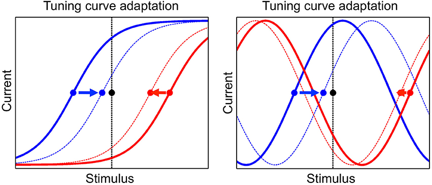
Figure 2. The adaptation mechanism, by which tuning curves of neurons are modified according to the presented stimulus. Tuning curves of two neurons are shown, one neuron in blue and the other one in red, before and after adaptation (full and dashed line, respectively). The presented stimulus is indicated by the black dot and the vertical black line. The tuning offsets of the two neurons are shown by the blue and red dots. Tuning offsets are attracted by the stimulus, as shown by the arrows. Left: sigmoidal tuning curves. Right: periodic tuning curves.

The dynamics of tuning offsets, Equation (8), implies that they are attracted by the presented stimulus, more so if they are closer to it (see Figure 2). For convenience, tuning offsets are reordered at each time step such that μ₁ < … < μ_N. Namely, after each update by Equation (8), if μ_i < μ_j for i > j then μ_i → μ_j and μ_j → μ_i (no other neural parameters are permuted in this step). Learning works without the permutation step but simplifies its implementation.

The spontaneous dynamics of the network is tested 10 times in each simulation, at fixed intervals of T/10 trials, referred to as 10 sessions. In each session of the spontaneous stage, external current, plasticity and adaptation are turned off, and the internal current is turned on. Recurrent neural dynamics is simulated with a time step Δt that is different from the one used during the stimulus-driven stage. In the stimulus driven stage, Δt reflects the presentation of a stimulus, which may occur on a time interval of a few seconds, while Δt in the spontaneous stage reflects the fast interaction between neurons through the internal currents, of the order of tens of milliseconds. This internal dynamics is implemented, by running Equations (2), (5), until the network reaches a stable fixed point, when neural activity does not change from one time step to the next. Then, this stable state is recorded and the stimulus driven dynamics is resumed until the next session.

Across the 10 sessions of one simulation, the stable state may change as a consequence of the changes in synapses occurred during the stimulus-driven stage. I show in the Appendix that the stable state must have a specific form that depends on a single parameter ν (see Appendix: “The spontaneous dynamics of neurons”). In general, this function is denoted by ξ(ν, μ_i) and, for a sigmoidal tuning curve, that is equal to

$\begin{array}{cc}{x}_i=\xi ({\mu }_i,\nu )=\text{sign}(\nu -{\mu }_i)& (10)\end{array}$

where ν is defined as the “retrieved” pattern and is sufficient to identify the entire network state. This form implies that the spontaneous state is equal to a pattern that would be obtained in presence of stimulus α = ν. In order to explore the possibility of the existence of multiple stable states, I run several simulations each one with a different initial condition, varying across the possible values of retrieved patterns.

The model has three parameters, N, T, and τ, fixed in each simulation. I used N = 1000 in most simulations, with a few simulations implementing N = 2000, 4000, 8000, and 16000. Three values of T used in simulations are T = 1000, T = 10000, and T = 100000. Three values of τ used in simulations are τ = 100, τ = 1000, and τ = 10000.

3. Results

A simulation of neural circuit dynamics is divided in two separate stages: a stimulus-driven stage and a spontaneous stage. During the stimulus-driven stage, sensory stimuli are presented and the external currents dominates over the internal currents. The response of a neuron to external stimuli is characterized by the tuning curve of that neuron (illustrated in Figure 1). During the spontaneous stage, there is no sensory stimulus and the neural circuit activates autonomously according to its internal currents. Synaptic plasticity and sensory adaptation occur during the stimulus-driven stage. Synaptic plasticity is implemented by a simple Hebbian rule, while sensory adaptation is implemented by modifying the tuning curve of neurons (illustrated in Figure 2). In each simulation, 10 sessions of stimulus-driven dynamics alternate with 10 sessions of spontaneous dynamics (see Materials and Methods for details).

Synaptic strengths are initialized at random, and they start switching as a result of plasticity, depending on the neural patterns of activity enforced by the presentation of stimuli. Upon presentation of a given stimulus, synaptic plasticity tends to make the corresponding neural activity pattern more stable, because of the Hebbian rule. A series of different stimuli are subsequently presented, determining a series of corresponding neural activity patterns. Therefore, because of the presentation of multiple stimuli, each pattern competes with other patterns for switching synapses in its own favor.

However, neural activity patterns not only compete but they also cooperate. Since the tuning curves of neurons are smooth functions of the stimulus (Figure 1), two similar values of the stimulus corresponds to two neural activity patterns that are also similar. Therefore, neural activity patterns are correlated, and two similar patterns collaborate in switching synapses toward stabilizing both of them. The resolution of this competition-cooperation trade-off depends on the distribution of input stimuli. If a subset of nearby stimuli is presented more often than other stimuli, the corresponding neural activity patterns will stabilize at the expense of others.

In order to determine which neural activity patterns stabilize as a consequence of synaptic plasticity, I measure the stable fixed points of the spontaneous dynamics, also referred to as “attractors” or “stable states.” At ten regular intervals (sessions) in each simulation, the stream of external stimuli is interrupted and the spontaneous dynamics is tested in presence of the internal currents only. This dynamics runs until the network reaches a stable fixed point, a neural activity pattern that does not change unless the system is perturbed. In each session, the spontaneous dynamics runs multiple times, with different initial conditions, to test for multiple stable states. After recording all the stable states, the stimulus-driven dynamics is resumed until the next session. The process is repeated for the 10 sessions of each simulation (see Materials and Methods).

The neural activity pattern corresponding to a given stable state is summarized by a single parameter, the “retrieved pattern.” This corresponds to the stimulus that, when presented, elicits exactly that neural pattern of activity. During the spontaneous dynamics there is no presentation of any stimulus, nevertheless the stable state is equivalent to the pattern elicited by that stimulus. The fact that the spontaneous dynamics reproduces the activity corresponding to a stimulus implies that synaptic plasticity has previously worked toward stabilizing that stimulus. I show in the Appendix (section: “The spontaneous dynamics of neurons”) that a spontaneous state is equal to a stimulus pattern provided that stimulus-driven synaptic plasticity has occurred for a time long enough.

Figure 3 shows the stable states (retrieved patterns), recorded during 10 subsequent sessions of spontaneous dynamics (ten rows, from top to bottom), plotted together with the distribution of input stimuli (top curve), in four different simulations (four panels). In each simulation, a different probability density p(α) is used to draw the sequence of input stimuli. Stimuli that are located near the highest mode of the distribution are more likely to be presented. Therefore, the corresponding neural activity patterns occur more often, and drive synaptic plasticity toward their own stabilization. As a consequence, in the first session one attractor state appears near the highest mode of the distribution (top row). In one simulation, two attractors appear near the highest mode. In another simulation, two attractor states appear, one near the highest mode, and another one near the second highest.

FIGURE 3

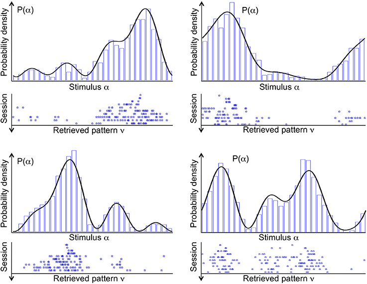
Figure 3. Distribution of stimuli p(α) (probability density, black curve) from which the sequence of input stimuli is drawn, and the stable fixed points of the spontaneous dynamics (attractors, blue stars), referred to as “retrieved patterns.” Four example simulations are shown in the four panels. Each stable fixed point is denoted by a star along the stimulus space. Different rows in each panel correspond to the 10 sessions of that simulation, ordered from top to bottom. In early sessions, a few attractors tend to locate near the modes of the probability density. In late sessions, several attractors sample the entire space of stimuli in proportion to the their likelihood. A histogram of the attractors from 1000 sessions (blue bars) is supermposed to the probability density of stimuli.

The landscape of attractor states changes significantly in ten subsequent sessions (Figure 3, ten rows, from top to bottom). First of all, attractor states are not maintained. If a given state is an attractor in one session, it is not necessarily an attractor in the next session. This is a consequence of the ongoing synaptic plasticity and the ongoing presentation of stimuli. Both processes are noisy: synaptic transitions are stochastic, and stimuli are drawn at random from the given probability density p(α). Most importantly, the number of attractor states increases significantly in subsequent sessions. In each simulation, the first session has only one or at most two attractor states. Numerous attractor states appear in subsequent sessions, which seems to sample precisely the distribution of input stimuli.

In summary, spontaneous activity of the neural circuit shows a large number of stable states which samples exactly the distribution of input stimuli. Therefore, spontaneous activity tends to linger on neural activity patterns that corresponds to specific input stimuli, more so if those stimuli have been experienced more often. Formally, spontaneous neural activity stops at a stable state and stays there indefinitely. However, in presence of noise, spontaneous activity would jump between attractor states (Amit, 1992), and would spend more time where a larger number of attractor states are present. In addition, I show below that an infinite number of stable fixed points (a continuous attractor) develops in the limit of an infinite number of neurons, implying that spontaneous activity is virtually free to sample the distribution. This property makes the neural circuit akin to a generative model of the stimuli (see Discussion).

The increase in the number of attractor states is a consequence of adaptation, as illustrated in Figure 4. Initially, synapses tend to favor neural activity patterns of stimuli that are encountered more often. However, adaptation tends to counterbalance this effect. In order to illustrate this, I associate each stimulus with a specific region of the neural circuit: when a stimulus is equal to the tuning offset of a neuron, I associate the stimulus with the location of that neuron. In Figure 4 (left), most stimuli are presented (gray shading) in the top left part of the network (therefore, most stimuli are equal to the tuning offsets of neurons in that part). As a consequence of adaptation, tuning offsets of neurons also tend to concentrate in that part of the network. This is illustrated by the external arrows that, representing fixed shapes of tuning curves, are “repelled” by those stimuli (right). The new organization of neurons following this transformation implies that the distribution of input stimuli now looks uniform (gray shading). I show in the Appendix that the distribution of tuning offsets of neurons matches exactly the distribution of presented stimuli (see Appendix: “The dynamics of tuning offsets”).

FIGURE 4

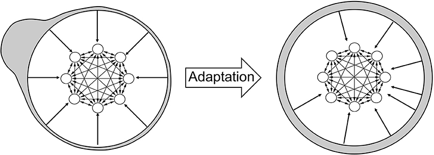
Figure 4. Effect of adaptation on the representation of stimuli. Left: illustration of the neural circuit model, same as in Figure 1. The tuning curves of different neurons are not shown here, but are still represented by the arrows pointing from the external circle to the neural circuit. The gray shading illustrates the distribution of external stimuli according to the network selectivity: the bump on the top left of the figure implies that most stimuli are presented in that region. By definition, a stimulus presented at a given place of the neural circuit is intended as equal to the tuning offset of the corresponding neuron. Right: after adaptation, the tuning curves of neurons are changed, as shown by the displacement of the arrows from the bulk of the stimulus distribution. As a consequence, the stimulus distribution in gray shading now appears uniform across the network (uniform gray shading around the circle).

Therefore, the network effectively “sees” a uniform distribution of presented stimuli. When synaptic plasticity applies to this uniform distribution, no specific stimulus pattern is favored with respect to any other. Therefore, the distribution of synaptic strengths do not favor any specific stimulus, and all patterns are equally likely to represent an attractor state. The increase in the number of attractors across sessions reflects the fact that synaptic plasticity tends to make more and more patterns suitable for stability. However, due to the finite size of the network, the stochastic synaptic transitions and the random presentation of stimuli, some neural patterns are still more likely than others to stabilize. Note that attractors distribute uniformly in the neural space, but since the neural representation of stimuli has changed, via the change in tuning curves, the attractors follows the distribution of stimuli in the stimulus space (see Discussion) as shown in Figure 3.

Figure 5 (left) shows the number of attractor states as a function of session for three different values of the timescale τ of plasticity and adaptation (both phenomena are assumed to evolve according to the same time constant τ). As described above, the number of attractor states increases in subsequent sessions. In addition, the number of attractor states also increases as a function of the timescale τ. A larger timescale implies a smaller effect of noise, because changes in synaptic strengths and tuning curves are slow enough to encompass a large number of stimulus presentations and average out the resulting fluctuations.

FIGURE 5

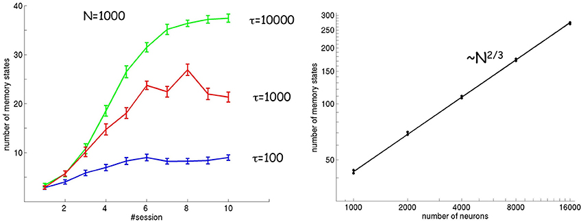
Figure 5. Number of attractor states as a function of session number, timescale τ (left), and number of neurons (right). The number of attractor states increases in subsequent sessions and for slower timescales. The scaling of the number of attractors with respect to the number of neurons is ~N^2/3.

In order for the spontaneous activity to match exactly the distribution of input stimuli, the landscape of attractor states should converge to an infinite number of fixed points (a continuous attractor) in the limit of a large number of neurons. I tested this hypothesis by looking at how the number of attractor states scales with the number of neurons. The result is shown in Figure 5 (right), where the number of attractor states is calculated in the limit of large τ and in stationary conditions. The number of attractor states increases as a function of the number of neurons according to a power law ~N^2/3. Using mathematical arguments, I show in the Appendix that in the limit of large N and τ, the dynamics indeed converges to a continuous (line) attractor state (see Appendix: “The spontaneous dynamics of neurons”).

4. Discussion

It is well known that Hebbian synaptic plasticity determines stable and autonomous neural patterns of activity, sometimes called “cell assemblies,” or “attractors” (Hopfield, 1982; Bernacchia and Amit, 2007). These stable states are spontaneous, since they can activate in absence of an external stimulus. In this work, I showed that if sensory adaptation is added to synaptic plasticity, these spontaneous states replicate the activity evoked by the previously experienced stimuli, in proportion to their relative occurrence. In other words, this set of stable states samples precisely the distribution of stimuli, and the neural circuit represents a generative model of the input stimuli (Hinton, 2007, 2010; Fiser et al., 2010; Barra et al., 2012; Clark, 2013). This is consistent with the observation that spontaneous activity of neurons in visual cortex reproduces the stimulus-evoked activity (Kenet et al., 2003; Berkes et al., 2011). According to Bayesian models, neural activity may represent the prior distribution of stimuli, either by encoding the value of the probability (Pouget et al., 2003), or by sampling that distribution (Hoyer and Hyvarinen, 2003). The present work is more consistent with the latter interpretation.

Bayesian models have been applied to a broad variety of problems in Neuroscience (Vilares and Kording, 2011), including multi-sensory integration (Ernst and Bülthoff, 2004; Knill and Pouget, 2004), sensory-motor control and action selection (Körding and Wolpert, 2006; Berniker et al., 2011). Bayesian models propose that neural circuits maintain a representation of the probability distribution of sensory stimuli (prior), and combine this prior distribution with new incoming information (Fiser et al., 2010). Probability distributions are believed to be represented by the activity of populations of neurons (Pouget et al., 2003). However, while the neural mechanisms of multi-sensory integration are starting to be elucidated (Stein and Stanford, 2008; Angelaki et al., 2009), it remains unknown how the brain forms priors and how it combines them with new information (Vilares and Kording, 2011).

The model studied in this work is characterized by binary neurons and binary synapses, and includes a simple model of sensory adaptation and synaptic plasticity. Because of its simplicity, the model does not account for a range of biological phenomena observed in real neurons and synapses, and any comparison between the model and experimental data may be only qualitative. However, the model can be easily simulated and analyzed, and the results can be understood in a formal mathematical framework. Details of the mathematical analysis of the model are developed in the Appendix. It remains to be tested whether the qualitative conclusions afforded by the model may be generalized to biologically more realistic situations.

A couple of groups studied more realistic neural circuit models including synaptic plasticity and spike-frequency adaptation, and showed that they optimize information transmission (Hennequin et al., 2010), and reproduce visual responses (Zylberberg et al., 2011). However, spike-frequency adaptation is different from the adaptation studied in this work, which is usually referred to as “sensory adaptation” (Wark et al., 2007; Gutkin and Zeldenrust, 2014). Sensory adaptation is a more general phenomenon, and spike-frequency adaptation is one of several possible mechanisms by which it is implemented in neural systems. In this work, I consider sensory adaptation without referring to any specific biological mechanism. This is expressed as a change in the tuning curve of neurons according to the adapting stimulus. In particular, I consider the attraction of the tuning curve by the adapting stimulus, which has been ubiquitously observed in the case of monotonic tuning curves (e.g., sigmoidal, Kohn, 2007; Rieke and Rudd, 2009). In case of unimodal tuning curves (e.g., sine), both repulsion (Müller et al., 1999; Dragoi et al., 2000) and attraction (Kohn and Movshon, 2004) of the tuning curve by the adapting stimulus has been observed. However, note that repulsion and attraction in those cases is meant with respect to the “preferred stimulus” of a neuron, instead of the “tuning offset.” In the present model, both repulsion and attraction can be observed with respect to the preferred stimulus (see e.g., Figure 2).

A substantial assumption of this work is that the representation of the stimulus follows the change in the tuning curves of neurons. In other words, a given neural activity pattern that represents a given stimulus at some moment in time, may represent a different stimulus later, because tuning curves of neurons have changed. In other words, I assume that the “homunculus” is “aware” of adaptation, while perceptual changes seem to be consistent with an “unaware” homunculus (Seriès et al., 2009), leading to what has been previously referred to as a decoding ambiguity (Fairhall et al., 2001), or coding catastrophe (Schwartz et al., 2007). However, behavioral and physiological observations are also consistent with a homunculus that is initially unaware of adaptation, but slowly catches up after enough time has passed since changes in stimulus encoding. In the present work, this could be modeled by using a faster timescale for adaptation and a slower timescale for plasticity. Future work will investigate the effects of changes in those timescales on the network dynamics and the attractor landscape (Chaudhuri et al., 2014).

In the present model, spontaneous activity converges to an attractor, a stable state of the neural dynamics and, by definition, it stays there indefinitely. However, in presence of noise, neural activity jumps between attractors (Amit, 1992), and the dynamics visits the different attractor states equally often. Furthermore, I showed that in the limit of an infinite number of neurons, the set of attractor states becomes infinite and converges to a continuous (line) attractor spanning the entire stimulus set. In that limit, the dynamics of neurons would not display discrete jumps, rather it would sample exactly and uniformly the continuous space of attractors.

As a final remark, note that in addition to representing a generative model of input stimuli, the model described here represents a solution to the problem of developing a continuous attractor from a set of discrete attractors, as previously investigated by Koulakov et al. (2002), Renart et al. (2003), Blumenfeld et al. (2006), Itskov et al. (2011).

Conflict of Interest Statement

The authors declare that the research was conducted in the absence of any commercial or financial relationships that could be construed as a potential conflict of interest.

Acknowledgments

The author would like to acknowledge Florin Ionita, Dong Li, Carlotta Martelli, and Benjamin Staar for useful comments on an earlier version of the manuscript.

References

Abbott, L. (2008). Theoretical neuroscience rising. Neuron 60, 489–495. doi: 10.1016/j.neuron.2008.10.019

Pubmed Abstract | Pubmed Full Text | CrossRef Full Text | Google Scholar

Abbott, L. F., and Nelson, S. B. (2000). Synaptic plasticity: taming the beast. Nat. Neurosci. 3, 1178–1183. doi: 10.1038/81453

Pubmed Abstract | Pubmed Full Text | CrossRef Full Text | Google Scholar

Amit, D. J. (1992). Modeling Brain Function: The World of Attractor Neural Networks. Cambridge, UK: Cambridge University Press.

Google Scholar

Angelaki, D. E., Gu, Y., and DeAngelis, G. C. (2009). Multisensory integration: psychophysics, neurophysiology, and computation. Curr. Opin. Neurobiol. 19, 452–458. doi: 10.1016/j.conb.2009.06.008

Pubmed Abstract | Pubmed Full Text | CrossRef Full Text | Google Scholar

Barra, A., Bernacchia, A., Santucci, E., and Contucci, P. (2012). On the equivalence of hopfield networks and boltzmann machines. Neural Netw. 34, 1–9. doi: 10.1016/j.neunet.2012.06.003

Pubmed Abstract | Pubmed Full Text | CrossRef Full Text | Google Scholar

Berkes, P., Orbán, G., Lengyel, M., and Fiser, J. (2011). Spontaneous cortical activity reveals hallmarks of an optimal internal model of the environment. Science 331, 83–87. doi: 10.1126/science.1195870

Pubmed Abstract | Pubmed Full Text | CrossRef Full Text | Google Scholar

Bernacchia, A., and Amit, D. J. (2007). Impact of spatiotemporally correlated images on the structure of memory. Proc. Natl. Acad. Sci. U.S.A. 104, 3544–3549. doi: 10.1073/pnas.0611395104

Pubmed Abstract | Pubmed Full Text | CrossRef Full Text | Google Scholar

Bernacchia, A., and Wang, X.-J. (2013). Decorrelation by recurrent inhibition in heterogeneous neural circuits. Neural Comput. 25, 1732–1767. doi: 10.1162/NECO-a-00451

Pubmed Abstract | Pubmed Full Text | CrossRef Full Text | Google Scholar

Berniker, M., Wei, K., and Kording, K. (2011). “Bayesian approaches to modelling action selection,” in Modelling Natural Action Selection, eds A. K. Seth, T. J. Prescott, and J. J. Bryson (Cambridge: Cambridge University Press), 120–143. doi: 10.1017/CBO9780511731525.010

CrossRef Full Text | Google Scholar

Bi, G.-Q., and Poo, M.-M. (2001). Synaptic modification by correlated activity: Hebb's postulate revisited. Ann. Rev. Neurosci. 24, 139–166. doi: 10.1146/annurev.neuro.24.1.139

Pubmed Abstract | Pubmed Full Text | CrossRef Full Text | Google Scholar

Blum, K. I., and Abbott, L. (1996). A model of spatial map formation in the hippocampus of the rat. Neural Comput. 8, 85–93. doi: 10.1162/neco.1996.8.1.85

Pubmed Abstract | Pubmed Full Text | CrossRef Full Text | Google Scholar

Blumenfeld, B., Preminger, S., Sagi, D., and Tsodyks, M. (2006). Dynamics of memory representations in networks with novelty-facilitated synaptic plasticity. Neuron 52, 383–394. doi: 10.1016/j.neuron.2006.08.016

Pubmed Abstract | Pubmed Full Text | CrossRef Full Text | Google Scholar

Borst, A., Flanagin, V. L., and Sompolinsky, H. (2005). Adaptation without parameter change: dynamic gain control in motion detection. Proc. Natl. Acad. Sci. U.S.A. 102, 6172–6176. doi: 10.1073/pnas.0500491102

Pubmed Abstract | Pubmed Full Text | CrossRef Full Text | Google Scholar

Brenner, N., Bialek, W., and de Ruyter van Steveninck, R. (2000). Adaptive rescaling maximizes information transmission. Neuron 26, 695–702. doi: 10.1016/S0896-6273(00)81205-2

Pubmed Abstract | Pubmed Full Text | CrossRef Full Text | Google Scholar

Buonomano, D. V., and Merzenich, M. M. (1998). Cortical plasticity: from synapses to maps. Ann. Rev. Neurosci. 21, 149–186. doi: 10.1146/annurev.neuro.21.1.149

Pubmed Abstract | Pubmed Full Text | CrossRef Full Text | Google Scholar

Calabresi, P., Picconi, B., Tozzi, A., and Di Filippo, M. (2007). Dopamine-mediated regulation of corticostriatal synaptic plasticity. Trends Neurosci. 30, 211–219. doi: 10.1016/j.tins.2007.03.001

Pubmed Abstract | Pubmed Full Text | CrossRef Full Text | Google Scholar

Caporale, N., and Dan, Y. (2008). Spike timing-dependent plasticity: a hebbian learning rule. Ann. Rev. Neurosci. 31, 25–46. doi: 10.1146/annurev.neuro.31.060407.125639

Pubmed Abstract | Pubmed Full Text | CrossRef Full Text | Google Scholar

Chaudhuri, R., Bernacchia, A., and Wang, X.-J. (2014). A diversity of localized timescales in network activity. eLife 3:e01239. doi: 10.7554/eLife.01239

Pubmed Abstract | Pubmed Full Text | CrossRef Full Text | Google Scholar

Clark, A. (2013). Whatever next? predictive brains, situated agents, and the future of cognitive science. Behav. Brain Sci. 36, 181–204. doi: 10.1017/S0140525X12000477

Pubmed Abstract | Pubmed Full Text | CrossRef Full Text | Google Scholar

Clifford, C. W., Webster, M. A., Stanley, G. B., Stocker, A. A., Kohn, A., Sharpee, T. O., et al. (2007). Visual adaptation: neural, psychological and computational aspects. Vision Res. 47, 3125–3131. doi: 10.1016/j.visres.2007.08.023

Pubmed Abstract | Pubmed Full Text | CrossRef Full Text | Google Scholar

Daw, N. D., and Doya, K. (2006). The computational neurobiology of learning and reward. Curr. Opin. Neurobiol. 16, 199–204. doi: 10.1016/j.conb.2006.03.006

Pubmed Abstract | Pubmed Full Text | CrossRef Full Text | Google Scholar

Dean, I., Harper, N. S., and McAlpine, D. (2005). Neural population coding of sound level adapts to stimulus statistics. Nat. Neurosci. 8, 1684–1689. doi: 10.1038/nn1541

Pubmed Abstract | Pubmed Full Text | CrossRef Full Text | Google Scholar

Doya, K. (2007). Reinforcement learning: computational theory and biological mechanisms. HFSP J 1, 30–40. doi: 10.2976/1.2732246/10.2976/1

Pubmed Abstract | Pubmed Full Text | CrossRef Full Text | Google Scholar

Dragoi, V., Sharma, J., and Sur, M. (2000). Adaptation-induced plasticity of orientation tuning in adult visual cortex. Neuron 28, 287–298. doi: 10.1016/S0896-6273(00)00103-3

Pubmed Abstract | Pubmed Full Text | CrossRef Full Text | Google Scholar

Ernst, M. O., and Bülthoff, H. H. (2004). Merging the senses into a robust percept. Trends Cogn. Sci. 8, 162–169. doi: 10.1016/j.tics.2004.02.002

Pubmed Abstract | Pubmed Full Text | CrossRef Full Text | Google Scholar

Fairhall, A. L., Lewen, G. D., Bialek, W., and van Steveninck, R. R. D. R. (2001). Efficiency and ambiguity in an adaptive neural code. Nature 412, 787–792. doi: 10.1038/35090500

Pubmed Abstract | Pubmed Full Text | CrossRef Full Text | Google Scholar

Feldman, D. E. (2009). Synaptic mechanisms for plasticity in neocortex. Ann. Rev. Neurosci. 32, 33. doi: 10.1146/annurev.neuro.051508.135516

Pubmed Abstract | Pubmed Full Text | CrossRef Full Text | Google Scholar

Feldman, D. E., and Brecht, M. (2005). Map plasticity in somatosensory cortex. Science 310, 810–815. doi: 10.1126/science.1115807

Pubmed Abstract | Pubmed Full Text | CrossRef Full Text | Google Scholar

Fiete, I. R., Senn, W., Wang, C. Z., and Hahnloser, R. H. (2010). Spike-time-dependent plasticity and heterosynaptic competition organize networks to produce long scale-free sequences of neural activity. Neuron 65, 563–576. doi: 10.1016/j.neuron.2010.02.003

Pubmed Abstract | Pubmed Full Text | CrossRef Full Text | Google Scholar

Fiser, J., Berkes, P., Orbán, G., and Lengyel, M. (2010). Statistically optimal perception and learning: from behavior to neural representations. Trends Cogn. Sci. 14, 119–130. doi: 10.1016/j.tics.2010.01.003

Pubmed Abstract | Pubmed Full Text | CrossRef Full Text | Google Scholar

Gallistel, C., and Matzel, L. D. (2013). The neuroscience of learning: beyond the hebbian synapse. Annual Rev. Psychol. 64, 169–200. doi: 10.1146/annurev-psych-113011-143807

Pubmed Abstract | Pubmed Full Text | CrossRef Full Text | Google Scholar

Gerstner, W., Kempter, R., van Hemmen, J. L., Wagner, H., et al. (1996). A neuronal learning rule for sub-millisecond temporal coding. Nature 383, 76–78. doi: 10.1038/383076a0

Pubmed Abstract | Pubmed Full Text | CrossRef Full Text | Google Scholar

Gerstner, W., Sprekeler, H., and Deco, G. (2012). Theory and simulation in neuroscience. Science 338, 60–65. doi: 10.1126/science.1227356

Pubmed Abstract | Pubmed Full Text | CrossRef Full Text | Google Scholar

Gutkin, B., and Zeldenrust, F. (2014). Spike frequency adaptation. Scholarpedia 9, 30643. doi: 10.4249/scholarpedia.30643

CrossRef Full Text | Google Scholar

Hennequin, G., Gerstner, W., and Pfister, J.-P. (2010). Stdp in adaptive neurons gives close-to-optimal information transmission. Front. Comput. Neurosci. 4:143. doi: 10.3389/fncom.2010.00143

Pubmed Abstract | Pubmed Full Text | CrossRef Full Text | Google Scholar

Herz, A. V., Gollisch, T., Machens, C. K., and Jaeger, D. (2006). Modeling single-neuron dynamics and computations: a balance of detail and abstraction. Science 314, 80–85. doi: 10.1126/science.1127240

Pubmed Abstract | Pubmed Full Text | CrossRef Full Text | Google Scholar

Hinton, G. E. (2007). Learning multiple layers of representation. Trends Cogn. Sci. 11, 428–434. doi: 10.1016/j.tics.2007.09.004

Pubmed Abstract | Pubmed Full Text | CrossRef Full Text | Google Scholar

Hinton, G. E. (2010). Learning to represent visual input. Philos. Trans. R. Soc. B Biol. Sci. 365, 177–184. doi: 10.1098/rstb.2009.0200

Pubmed Abstract | Pubmed Full Text | CrossRef Full Text | Google Scholar

Hopfield, J. J. (1982). Neural networks and physical systems with emergent collective computational abilities. Proc. Natl Acad. Sci. U.S.A. 79, 2554–2558. doi: 10.1073/pnas.79.8.2554

Pubmed Abstract | Pubmed Full Text | CrossRef Full Text | Google Scholar

Hoyer, P. O., and Hyvarinen, A. (2003). Interpreting neural response variability as monte carlo sampling of the posterior. Adv. Neural Inf. Process. Syst. 293–300.

Google Scholar

Itskov, V., Hansel, D., and Tsodyks, M. (2011). Short-term facilitation may stabilize parametric working memory trace. Front. Comput. Neurosci. 5:40. doi: 10.3389/fncom.2011.00040

Pubmed Abstract | Pubmed Full Text | CrossRef Full Text | Google Scholar

Katz, L. C., and Shatz, C. J. (1996). Synaptic activity and the construction of cortical circuits. Science 274, 1133–1138. doi: 10.1126/science.274.5290.1133

Pubmed Abstract | Pubmed Full Text | CrossRef Full Text | Google Scholar

Kenet, T., Bibitchkov, D., Tsodyks, M., Grinvald, A., and Arieli, A. (2003). Spontaneously emerging cortical representations of visual attributes. Nature 425, 954–956. doi: 10.1038/nature02078

Pubmed Abstract | Pubmed Full Text | CrossRef Full Text | Google Scholar

Knill, D. C., and Pouget, A. (2004). The bayesian brain: the role of uncertainty in neural coding and computation. Trends Neurosci. 27, 712–719. doi: 10.1016/j.tins.2004.10.007

Pubmed Abstract | Pubmed Full Text | CrossRef Full Text | Google Scholar

Kohn, A. (2007). Visual adaptation: physiology, mechanisms, and functional benefits. J. Neurophysiol. 97, 3155–3164. doi: 10.1152/jn.00086.2007

Pubmed Abstract | Pubmed Full Text | CrossRef Full Text | Google Scholar

Kohn, A., and Movshon, J. A. (2004). Adaptation changes the direction tuning of macaque mt neurons. Nat. Neurosci. 7, 764–772. doi: 10.1038/nn1267

Pubmed Abstract | Pubmed Full Text | CrossRef Full Text | Google Scholar

Körding, K. P., and Wolpert, D. M. (2006). Bayesian decision theory in sensorimotor control. Trends Cogn. Sci. 10, 319–326. doi: 10.1016/j.tics.2006.05.003

Pubmed Abstract | Pubmed Full Text | CrossRef Full Text | Google Scholar

Koulakov, A. A., Raghavachari, S., Kepecs, A., and Lisman, J. E. (2002). Model for a robust neural integrator. Nat. Neurosci. 5, 775–782. doi: 10.1038/nn893

Pubmed Abstract | Pubmed Full Text | CrossRef Full Text | Google Scholar

Krekelberg, B., Van Wezel, R. J., and Albright, T. D. (2006). Adaptation in macaque mt reduces perceived speed. J. Neurophysiol. 95, 255–270. doi: 10.1152/jn.00750.2005

Pubmed Abstract | Pubmed Full Text | CrossRef Full Text | Google Scholar

Lamprecht, R., and LeDoux, J. (2004). Structural plasticity and memory. Nat. Rev. Neurosci. 5, 45–54. doi: 10.1038/nrn1301

Pubmed Abstract | Pubmed Full Text | CrossRef Full Text | Google Scholar

Laughlin, S. B. (1981). A simple coding procedure enhances a neurons information capacity. Z. Naturforsch 36, 51.

Pubmed Abstract | Pubmed Full Text | Google Scholar

Machens, C. K., Gollisch, T., Kolesnikova, O., and Herz, A. V. (2005). Testing the efficiency of sensory coding with optimal stimulus ensembles. Neuron 47, 447–456. doi: 10.1016/j.neuron.2005.06.015

Pubmed Abstract | Pubmed Full Text | CrossRef Full Text | Google Scholar

Maravall, M., Petersen, R. S., Fairhall, A. L., Arabzadeh, E., and Diamond, M. E. (2007). Shifts in coding properties and maintenance of information transmission during adaptation in barrel cortex. PLoS Biol. 5:e19. doi: 10.1371/journal.pbio.0050019

Pubmed Abstract | Pubmed Full Text | CrossRef Full Text | Google Scholar

Martin, S., Grimwood, P., and Morris, R. (2000). Synaptic plasticity and memory: an evaluation of the hypothesis. Ann. Rev. Neurosci. 23, 649–711. doi: 10.1146/annurev.neuro.23.1.649

Pubmed Abstract | Pubmed Full Text | CrossRef Full Text | Google Scholar

Mehta, M., Lee, A., and Wilson, M. (2002). Role of experience and oscillations in transforming a rate code into a temporal code. Nature 417, 741–746. doi: 10.1038/nature00807

Pubmed Abstract | Pubmed Full Text | CrossRef Full Text | Google Scholar

Miller, K. D. (1996). Synaptic economics: competition and cooperation in synaptic plasticity. Neuron 17, 371–374. doi: 10.1016/S0896-6273(00)80169-5

Pubmed Abstract | Pubmed Full Text | CrossRef Full Text | Google Scholar

Montague, P. R., Hyman, S. E., and Cohen, J. D. (2004). Computational roles for dopamine in behavioural control. Nature 431, 760–767. doi: 10.1038/nature03015

Pubmed Abstract | Pubmed Full Text | CrossRef Full Text | Google Scholar

Müller, J. R., Metha, A. B., Krauskopf, J., and Lennie, P. (1999). Rapid adaptation in visual cortex to the structure of images. Science 285, 1405–1408. doi: 10.1126/science.285.5432.1405

Pubmed Abstract | Pubmed Full Text | CrossRef Full Text | Google Scholar

Nagel, K. I., and Doupe, A. J. (2006). Temporal processing and adaptation in the songbird auditory forebrain. Neuron 51, 845–859. doi: 10.1016/j.neuron.2006.08.030

Pubmed Abstract | Pubmed Full Text | CrossRef Full Text | Google Scholar

Ohzawa, I., Sclar, G., and Freeman, R. D. (1985). Contrast gain control in the cats visual system. J. Neurophysiol. 54, 651–667.

Pubmed Abstract | Pubmed Full Text | Google Scholar

Pawlak, V., Wickens, J. R., Kirkwood, A., and Kerr, J. N. (2010). Timing is not everything: neuromodulation opens the stdp gate. Front. Synaptic Neurosci. 2:146. doi: 10.3389/fnsyn.2010.00146

Pubmed Abstract | Pubmed Full Text | CrossRef Full Text | Google Scholar

Pouget, A., Dayan, P., and Zemel, R. S. (2003). Inference and computation with population codes. Ann. Rev. Neurosci. 26, 381–410. doi: 10.1146/annurev.neuro.26.041002.131112

Pubmed Abstract | Pubmed Full Text | CrossRef Full Text | Google Scholar

Renart, A., Song, P., and Wang, X.-J. (2003). Robust spatial working memory through homeostatic synaptic scaling in heterogeneous cortical networks. Neuron 38, 473–485. doi: 10.1016/S0896-6273(03)00255-1

Pubmed Abstract | Pubmed Full Text | CrossRef Full Text | Google Scholar

Rieke, F., and Rudd, M. E. (2009). The challenges natural images pose for visual adaptation. Neuron 64, 605–616. doi: 10.1016/j.neuron.2009.11.028

Pubmed Abstract | Pubmed Full Text | CrossRef Full Text | Google Scholar

Royer, S., and Paré, D. (2003). Conservation of total synaptic weight through balanced synaptic depression and potentiation. Nature 422, 518–522. doi: 10.1038/nature01530

Pubmed Abstract | Pubmed Full Text | CrossRef Full Text | Google Scholar

Sakmann, B., and Creutzfeldt, O. D. (1969). Scotopic and mesopic light adaptation in the cat's retina. Pflügers Arch. 313, 168–185. doi: 10.1007/BF00586245

Pubmed Abstract | Pubmed Full Text | CrossRef Full Text | Google Scholar

Sanes, J. R., and Lichtman, J. W. (1999). Development of the vertebrate neuromuscular junction. Ann. Rev. Neurosci. 22, 389–442. doi: 10.1146/annurev.neuro.22.1.389

Pubmed Abstract | Pubmed Full Text | CrossRef Full Text | Google Scholar

Savin, C., Joshi, P., and Triesch, J. (2010). Independent component analysis in spiking neurons. PLoS Comput. Biol. 6:e1000757. doi: 10.1371/journal.pcbi.1000757

Pubmed Abstract | Pubmed Full Text | CrossRef Full Text | Google Scholar

Schwartz, O., Hsu, A., and Dayan, P. (2007). Space and time in visual context. Nat. Rev. Neurosci. 8, 522–535. doi: 10.1038/nrn2155

Pubmed Abstract | Pubmed Full Text | CrossRef Full Text | Google Scholar

Seriès, P., Stocker, A. A., and Simoncelli, E. P. (2009). Is the homunculus aware of sensory adaptation? Neural Comput. 21, 3271–3304. doi: 10.1162/neco.2009.09-08-869

Pubmed Abstract | Pubmed Full Text | CrossRef Full Text | Google Scholar

Seung, H. S. (2003). Learning in spiking neural networks by reinforcement of stochastic synaptic transmission. Neuron 40, 1063–1073. doi: 10.1016/S0896-6273(03)00761-X

Pubmed Abstract | Pubmed Full Text | CrossRef Full Text | Google Scholar

Seung, H. S. (2009). Reading the book of memory: sparse sampling versus dense mapping of connectomes. Neuron 62, 17–29. doi: 10.1016/j.neuron.2009.03.020

Pubmed Abstract | Pubmed Full Text | CrossRef Full Text | Google Scholar

Shapley, R., and Enroth-Cugell, C. (1984). Visual adaptation and retinal gain controls. Prog. Retinal Res. 3, 263–346. doi: 10.1016/0278-4327(84)90011-7

CrossRef Full Text | Google Scholar

Smirnakis, S. M., Berry, M. J., Warland, D. K., Bialek, W., and Meister, M. (1997). Adaptation of retinal processing to image contrast and spatial scale. Nature 386, 69–73. doi: 10.1038/386069a0

Pubmed Abstract | Pubmed Full Text | CrossRef Full Text | Google Scholar

Soltani, A., and Wang, X.-J. (2008). From biophysics to cognition: reward-dependent adaptive choice behavior. Curr. Opin. Neurobiol. 18, 209–216. doi: 10.1016/j.conb.2008.07.003

Pubmed Abstract | Pubmed Full Text | CrossRef Full Text | Google Scholar

Song, S., and Abbott, L. F. (2001). Cortical development and remapping through spike timing-dependent plasticity. Neuron 32, 339–350. doi: 10.1016/S0896-6273(01)00451-2

Pubmed Abstract | Pubmed Full Text | CrossRef Full Text | Google Scholar

Stein, B. E., and Stanford, T. R. (2008). Multisensory integration: current issues from the perspective of the single neuron. Nat. Rev. Neurosci. 9, 255–266. doi: 10.1038/nrn2331

Pubmed Abstract | Pubmed Full Text | CrossRef Full Text | Google Scholar

Surmeier, D. J., Plotkin, J., and Shen, W. (2009). Dopamine and synaptic plasticity in dorsal striatal circuits controlling action selection. Curr. Opin. Neurobiol. 19, 621–628. doi: 10.1016/j.conb.2009.10.003

Pubmed Abstract | Pubmed Full Text | CrossRef Full Text | Google Scholar

Tetzlaff, C., Kolodziejski, C., Markelic, I., and Wörgötter, F. (2012). Time scales of memory, learning, and plasticity. Biol. Cybern. 106, 715–726. doi: 10.1007/s00422-012-0529-z

Pubmed Abstract | Pubmed Full Text | CrossRef Full Text | Google Scholar

Toyoizumi, T., Pfister, J.-P., Aihara, K., and Gerstner, W. (2005). Generalized bienenstock–cooper–munro rule for spiking neurons that maximizes information transmission. Proc. Natl. Acad. Sci. U.S.A. 102, 5239–5244. doi: 10.1073/pnas.0500495102

Pubmed Abstract | Pubmed Full Text | CrossRef Full Text | Google Scholar

Tsodyks, M. (1990). Associative memory in neural networks with binary synapses. Mod. Phys. Lett. B 4, 713–716. doi: 10.1142/S0217984990000891

CrossRef Full Text | Google Scholar

Turrigiano, G. G., and Nelson, S. B. (2004). Homeostatic plasticity in the developing nervous system. Nat. Rev. Neurosci. 5, 97–107. doi: 10.1038/nrn1327

Pubmed Abstract | Pubmed Full Text | CrossRef Full Text | Google Scholar

Vilares, I., and Kording, K. (2011). Bayesian models: the structure of the world, uncertainty, behavior, and the brain. Ann. N.Y. Acad. Sci. 1224, 22–39. doi: 10.1111/j.1749-6632.2011.05965.x

Pubmed Abstract | Pubmed Full Text | CrossRef Full Text | Google Scholar

Wainwright, M. J. (1999). Visual adaptation as optimal information transmission. Vision Res. 39, 3960–3974. doi: 10.1016/S0042-6989(99)00101-7

Pubmed Abstract | Pubmed Full Text | CrossRef Full Text | Google Scholar

Wark, B., Lundstrom, B. N., and Fairhall, A. (2007). Sensory adaptation. Curr. Opin. Neurobiol. 17, 423–429. doi: 10.1016/j.conb.2007.07.001

Pubmed Abstract | Pubmed Full Text | CrossRef Full Text | Google Scholar

Webster, M. A. (2011). Adaptation and visual coding. J. Vis. 11, 3. doi: 10.1167/11.5.3

Pubmed Abstract | Pubmed Full Text | CrossRef Full Text | Google Scholar

Wickens, J. R., Reynolds, J. N., and Hyland, B. I. (2003). Neural mechanisms of reward-related motor learning. Curr. Opin. Neurobiol. 13, 685–690. doi: 10.1016/j.conb.2003.10.013

Pubmed Abstract | Pubmed Full Text | CrossRef Full Text | Google Scholar

Williams, A. H., O'Leary, T., and Marder, E. (2013). Homeostatic regulation of neuronal excitability. Scholarpedia 8, 1656. doi: 10.4249/scholarpedia.1656

CrossRef Full Text | Google Scholar

Zylberberg, J., Murphy, J. T., and DeWeese, M. R. (2011). A sparse coding model with synaptically local plasticity and spiking neurons can account for the diverse shapes of v1 simple cell receptive fields. PLoS Comput. Biol. 7:e1002250. doi: 10.1371/journal.pcbi.1002250

Pubmed Abstract | Pubmed Full Text | CrossRef Full Text | Google Scholar

Appendix

In this section, I derive useful expressions of the following quantities: (1) The stationary distribution of synaptic strengths; (2) The stationary distribution of tuning offsets; (3) The stable states of the spontaneous dynamics. Those quantities are instrumental for understanding the results presented in the main text.

The Dynamics of Synaptic Strengths

Synaptic plasticity occurs during the presentation of input stimuli, and the statistics of those stimuli affect the synaptic strengths. The goal of this section is to derive a simple expression for the stationary average of synaptic strengths, as a function of the statistics of input stimuli.

The probability that at time t a synapse is potentiated (J_ij(t) = +1) is denoted by u(t). Conversely, the probability that the synapse is depressed (J_ij(t) = −1) is denoted by v(t). The normalization condition holds, namely

$\begin{array}{cc}u(t)+v(t)=1& (\text{A}1)\end{array}$

Using these probabilities, the average synaptic strength is equal to

$\begin{array}{cc}{\langle J_{ij}\rangle }_t=u(t)-v(t)& (\text{A2)}\end{array}$

The angular brackets denote an average over the distribution of synaptic stenghts. Using Equations (A1), (A2), the probabilities u(t), v(t) are written in terms of the average, i.e.,

$\begin{array}{cc}u(t)=\frac{1+{\langle J_{ij}\rangle }_t}{2}& (\text{A}3)\end{array}$

$\begin{array}{cc}v(t)=\frac{1-{\langle J_{ij}\rangle }_t}{2}& (\text{A}4)\end{array}$

In order to derive a master equation which describes the evolution of the average synaptic matrix 〈J_ij〉, transition probabilities must be defined. The probability of potentiation, namely the probability of the transition from J_ij(t) = −1 to J_ij(t + Δt) = +1 is denoted as w₊. Conversely, the probability of depression, namely the probability of the transition from J_ij(t) = +1 to J_ij(t + Δt) = −1 is denoted as w₋. The evolution of u(t) is given by the master equation

$\begin{array}{cc}u(t+\Delta t)-u(t)=w_{+}v(t)-w_{-}u(t)& (\text{A}5)\end{array}$

In words, the change in the fraction of potentiated synapses during a time step Δt is equal to the fraction of depressed synapses that are potentiated minus the fraction of potentiated synapses that are depressed in that time step. Substituting Equations (A3), (A4) into Equation (A5), it is possible to write the equation in terms of the average synaptic efficacy, namely

$\begin{array}{cc}{\langle J_{ij}\rangle }_{t+\Delta t}-{\langle J_{ij}\rangle }_t=-(w_{+}+w_{-}){\langle J_{ij}\rangle }_t+(w_{+}-w_{-})& (\text{A}6)\end{array}$

The transition probabilities depend on neural activity according to a Hebbian prescription, given by Equations (6), (7). Substituting those equations, the above Equation (A6) is rewritten as

$\begin{array}{cc}\tau \left[{\langle J_{ij}\rangle }_{t+\Delta t}-{\langle J_{ij}\rangle }_t\right]=-{\langle J_{ij}\rangle }_t+x_i(t)x_j(t)& (\text{A}7)\end{array}$

This equation shows how the average synaptic strength changes according to neural activity of the pre and post-synaptic neurons. For simplicity, in the following I use Δt = 1. The solution of Equation (A7) is equal to

$\begin{array}{cc}{\langle J_{ij}\rangle }_t\text{}=\text{}\frac{1}{\tau }{\displaystyle \sum _{t^{\prime }=0}^{t-1}{\left(1-\frac{1}{\tau }\right)}^{t-t^{\prime }-1}}{x}_i(t^{\prime })x_j(t^{\prime })+{\left(1-\frac{1}{\tau }\right)}^t{\langle J_{ij}\rangle }_0& (\text{A}8)\end{array}$

In the following, I assume that time t is large enough for the initial condition to decay away, namely t ≫ τ. Plasticity occurs during stimulus presentation, which imposes a specific pattern of neural activity. During presentation of stimulus α(t) at time t, neural activity is equal to

$\begin{array}{cc}{x}_i(t)=\xi ({\mu }_i,\alpha (t))& (\text{A}9)\end{array}$

Substituting Equation (A9) into Equation (A8), the expression of the average synaptic strengths is rewritten as

$\begin{array}{cc}{\langle J_{ij}\rangle }_t=\frac{1}{\tau }{\displaystyle \sum _{t^{\prime }=0}^{t-1}{\left(1-\frac{1}{\tau }\right)}^{t-t^{\prime }-1}}\xi ({\mu }_i,\alpha (t^{\prime }))\xi ({\mu }_j,\alpha (t^{\prime }))& (\text{A}10)\end{array}$

As explained in the Materials and Methods section, in each trial one stimulus α is drawn at random from a distribution p(α). In the limit of large t and τ (and t ≫ τ), the sum over t′ in Equation (A10) can be replaced by an integral over the distribution of the stimulus values, and the stationary synaptic strengths are equal to

$\begin{array}{cc}\langle J_{ij}\rangle ={\displaystyle {\int }_0^{1}d}\alpha p(\alpha )\xi ({\mu }_i,\alpha )\xi ({\mu }_j,\alpha )& (\text{A}11)\end{array}$

The Dynamics of Tuning Offsets

In addition to plasticity, during the presentation of input stimuli also adaptation takes place, and determines a change in the tuning offsets of neurons. The goal of this section is to derive a simple expression for the distribution of tuning offsets as a function of the statistics of input stimuli. The final result is that, under certain assumptions, the distribution of tuning offsets is equal to the distribution of input stimuli.

The dynamics of tuning offsets is defined by Equation (8). That equation is rewritten here with a minor rearrangement of terms

$\begin{array}{cc}\tau [{\mu }_i(t+\Delta t)-{\mu }_i(t)]={\mu }_i^0-\Theta ({\mu }_i(t)-\alpha (t))& (\text{A}12)\end{array}$

I assume that after enough time has passed, this dynamics settles into a stationary state. In particular, this assumption will be met in the limit of large τ. The stationary state is defined by the condition that the temporal average of μ_i(t + Δt) is equal to the temporal average of μ_i(t). In other words, the temporal average of the left hand side is zero. Therefore, the temporal average of the right hand side must be also zero. The temporal average of the Θ step function is equal to the fraction of times in which its argument is positive, namely the probability that μ_i > α. On the other hand, μ⁰_i is constant and given by Equation (9). Therefore, the stationary condition reads

$\begin{array}{cc}\text{Prob}({\mu }_i>\alpha )={\mu }_i^0=\frac{i-1/2}{N}& (\text{A}13)\end{array}$

Note that μ⁰_i represents an ordered and uniform tiling of the interval (0,1) by neurons. At the stationary state, when the values of μ_i are relatively fixed and stable, the left hand side is equal to the cumulative distribution function of the input stimuli α. I denote the density and cumulative distribution function of the input stimuli by, respectively, p(α) and P(α). Therefore, Equation (A13) is rewritten as

$\begin{array}{cc}P({\mu }_i)={\mu }_i^0& (\text{A}14)\end{array}$

By definition of cumulative distribution function, P can be inverted to obtain the tuning offsets of neurons

$\begin{array}{cc}{\mu }_i=P^{-1}({\mu }_i^0)& (\text{A}15)\end{array}$

In the limit of large N, I can substitute the index i with a label y = μ⁰_i spanning a continuum of neurons in the interval (0,1). Therefore,

$\begin{array}{cc}\mu (y)=P^{-1}(y)& (\text{A}16)\end{array}$

Then, it is easy to show that the tuning offsets of neurons follow the same distribution of input stimuli. By taking the derivative of Equation (A16) with respect to y, I can calculate the volume dy of neurons with tuning offsets included in a given interval dμ, that is equal to

$\begin{array}{cc}dy=p(\mu )d\mu & (\text{A}17)\end{array}$

Therefore, the density function of tuning offsets across neurons is equal to the p(μ), which is equal to the density of input stimuli. I denote the density of tuning offsets as g(μ) and the density of input stimuli as p(α). Therefore, the above result is written as

$\begin{array}{cc}g(\mu )=p(\mu )& (\text{A}18)\end{array}$

The Spontaneous Dynamics of Neurons

The goal of this section is to derive a simple equation describing the (stable) fixed points of the retrieval dynamics of neurons, that is the dynamics in absence of stimulus and plasticity. However, I assume that stimulation and plasticity have occurred before this retrieval stage, and synaptic strengths have been modified by the distribution of input stimuli through Equation (A11). Therefore, the distribution of input stimuli in turn affects the neural dynamics during retrieval. Neural dynamics also depends on the distribution of tuning offsets.

During the retrieval phase there is no input stimulus, therefore the total current I_i is equal to the internal current, given by Equation (5). In the limit of a large number of neurons N, I can substitute the synaptic strength J_ij with its average, therefore the current is equal to

$\begin{array}{cc}{I}_i(t)=\frac{1}{2N}{\displaystyle \sum _j\langle J_{ij}\rangle x_j(t)}& (\text{A}19)\end{array}$

I substitute the expression for the average synaptic strength, Equation (A11), into Equation (A19), and the new expression for the current is

$\begin{array}{cc}{I}_i(t)=\frac{1}{2N}{\displaystyle {\int }_0^{1}d}\alpha p(\alpha )\xi ({\mu }_i,\alpha ){\displaystyle \sum _{j=1}^N\xi }({\mu }_j,\alpha )x_j(t)& (\text{A}20)\end{array}$

As mentioned above, during the retrieval phase there is no input stimulus. Nevertheless, I assume that neural activity is equal to a pattern that would be obtained by stimulating the network with a given stimulus ν. Namely, I assume that

$\begin{array}{cc}{x}_j(t)=\xi ({\mu }_j,\nu (t))& (\text{A}21)\end{array}$

The value of ν depends on time and is unknown. This assumption is verified below by a self-consistent argument. Under this assumption, the new expression of the current is obtained by substituting Equation (A21) into Equation (A20), to find

$\begin{array}{cc}{I}_i=\frac{1}{2N}{\displaystyle {\int }_0^{1}d}\alpha p(\alpha )\xi ({\mu }_i,\alpha ){\displaystyle \sum _{j=1}^N\xi }({\mu }_j,\alpha )\xi ({\mu }_j,\nu )& (\text{A}22)\end{array}$

where I dropped the explicit dependence on time. In the limit of a large number of neurons N, I can substitute the sum over the index j with an integral over the tuning offsets of neurons, μ = μ_j, according to the distribution of such tuning offsets, which I denote by g(μ). Namely, I can use the following expression

$\begin{array}{cc}\frac{1}{N}{\displaystyle \sum _{j=1}^N\xi }({\mu }_j,\alpha )\xi ({\mu }_j,\nu )={\displaystyle {\int }_0^{1}d}\mu g(\mu )\xi (\mu ,\alpha )\xi (\mu ,\nu )& (\text{A}23)\end{array}$

By substituting Equation (A23) into Equation (A22), the new expression for the current is

$\begin{array}{cc}{I}_i=\frac{1}{2}{\displaystyle {\int }_0^{1}d}\alpha d\mu p(\alpha )g(\mu )\xi ({\mu }_i,\alpha )\xi (\mu ,\alpha )\xi (\mu ,\nu )& (\text{A}24)\end{array}$

This expression is useful for studying the stable states of neural dynamics. However, first the assumption made in Equation (A21) must be checked. The following analysis is valid in case of a sigmoidal tuning curve, Equation (3), which implies ξ(μ, ν) = sign(μ − ν), but similar results are obtained in case of a periodic tuning curve Equation (4).

The assumption in Equation (A21) states that neural activity in absence of the stimulus is equal to the activity in presence of a stimulus, for a given unknown stimulus ν at time t. In order to check this assumption, I follow a self-consistent argument: given that the assumption is true at time t, test whether it remains true at time t + Δt. In other words, given Equation (A21), it must be true that

$\begin{array}{cc}{x}_i(t+\Delta t)=\xi ({\mu }_i,\nu (t+\Delta t))& (\text{A}25)\end{array}$

Note that the ν(t + Δt) is not given and can be any value in the interval (0,1). Equation (A24) was derived under the assumption of Equation (A21), therefore I check whether Equation (A24) implies Equation (A25). I substitute the expression for the function ξ, Equation (10) in Equation (A24). After calculating the integral explicitly, I express the current in terms of the cumulative distribution functions of the input stimuli P and tuning offsets G, whose density functions are, respectively, p and g. The result is

$\begin{array}{l}{I}_i=G(\nu )-P({\mu }_i)+\frac{1}{2}{\displaystyle {\int }_0^{1}d}\alpha [P(\alpha )g(\alpha )-p(\alpha )G(\alpha )]+\text{sign}({\mu }_i-\nu )·\\ ·\left\{[P({\mu }_i)-P(\nu )][G({\mu }_i)-G(\nu )]+[P(\nu )G({\mu }_i)-P({\mu }_i)G(\nu )]-{\displaystyle {\int }_{\nu }^{{\mu }_i}d}\alpha [p(\alpha )G(\alpha )-P(\alpha )g(\alpha )]\right\}\end{array}$

Note that the term in curly brackets is small for μ_i ~ ν. In that case, the current is approximated by

$\begin{array}{cc}{I}_i\simeq G(\nu )-P({\mu }_i)+\frac{1}{2}{\displaystyle {\int }_0^{1}d}\alpha [P(\alpha )g(\alpha )-p(\alpha )G(\alpha )]& (\text{A}26)\end{array}$

This is a monotonically decreasing function of μ_i, because the cumulative distribution P is monotonically increasing by definition. In addition, the current I_i takes opposite values at the extreme points μ_i = 0 and μ_i = 1. Therefore, it must vanish at a unique value of μ_i, provided that this value is close enough to ν to justify the approximation μ_i ~ ν. I define this value as ν(t + Δt). As a consequence, using Equation (2), the neural activity is equal to

$\begin{array}{cc}{x}_i(t+\Delta t)=\text{sign}(I_i)=\text{sign}(\nu (t+\Delta t)-{\mu }_i)=\xi ({\mu }_i,\nu (t+\Delta t))& (\text{A}27)\end{array}$

and Equation (A25) is demonstrated. Therefore, the assumption that neural activity in absence of the stimulus takes the form of Equation (A21) is self-consistent. The value of ν(t + Δt) can be calculated as a function of the value of ν(t). Under the assumption that the two values are close, ν(t + Δt) ~ ν(t), this can be calculated by replacing μ_i with ν(t + Δt) in Equation (A26). Therefore,

$\begin{array}{cc}P(\nu (t+\Delta t))-G(\nu (t))+\frac{1}{2}{\displaystyle {\int }_0^{1}d}\alpha [p(\alpha )G(\alpha )-P(\alpha )g(\alpha )]=0& (\text{A}28)\end{array}$

In order to find the fixed points of neural activity, I impose that ν(t + Δt) = ν(t) = ν. The value of ν is the fixed point of the retrieval dynamics. This condition is equivalent to

$\begin{array}{cc}P(\nu )-G(\nu )+\frac{1}{2}{\displaystyle {\int }_0^{1}d}\alpha [p(\alpha )G(\alpha )-P(\alpha )g(\alpha )]=0& (\text{A}29)\end{array}$

This equation can be solved to find the fixed points ν for a given distribution of input stimuli p and of tuning offsets g. By taking the derivative of Equation (A28) with respect to ν, it is easy to check that a fixed point ν is stable if and only if

$\begin{array}{cc}p(\nu )>g(\nu )& (\text{A}30)\end{array}$

Note that if the two distributions p and g are exactly equal, as happens at the stationary state of the dynamics of tuning offsets, Equation (A18), then all possible values of ν correspond to marginally stable fixed points. This corresponds to a continuous attractor state.