A novel model-free data analysis technique based on clustering in a mutual information space: application to resting-state fMRI

Introduction

Conventional methodology of fMRI analysis has favored model-based approaches, where the fMRI signal is correlated with an estimated functional response model or where a statistical comparison between the control and activated states is performed (Chuang et al., 1999). The prime example is the general linear model used in the popular software packages SPM (Friston et al., 1995) and FSL (Smith et al., 2004). The construction and parametric fitting of a model inevitably involves limitations stemming from the adopted assumptions. Consequently, the analysis and its outcomes are restricted with respect to feasible experimental conditions and the complexity of the estimated response signals (Chuang et al., 1999).

On the other hand, the model-free approach provides scope for unsupervised, purely data-driven, and bias-free ways of investigating neuroimaging data. Its potential lies in the concept of exploratory multivariate search for specific signal features without imposing rigid limitations on their spatio-temporal form. Thus, since no assumed model of functional response is needed, more complex experimental paradigms and non-standard fMRI activation patterns can be studied.

One such non-standard fMRI experiment is the study of so-called resting-state networks. These originate from the fluctuations in brain activity when the subject is at rest and are thought to reflect the underlying connectivity of the brain (Smith et al., 2009). There have been a number of model-free methods suggested for this type of fMRI data analysis, where we distinguish between three different classes of methods below.

First, independent component analysis (ICA) is commonly used in fMRI data analysis and it assumes a predefined number of components of the activity patterns to be linearly statistically independent (McKeown et al., 1998). Also, to cope with the computational complexity the dimensionality of the input data is typically reduced by PCA (Beckmann et al., 2005). Second, in various partial correlation whole-brain analysis methods and seed voxel-based methods (Salvador et al., 2005), a number of areas of the brain are specified and correlations between these are calculated. Clustering can then be performed on the correlation relations between these small numbers of areas. Third, in clustering techniques, a predefined number of clusters are adapted to the data according to some statistical distance metric (Chuang et al., 1999), either directly on the input data (Golland et al., 2008) or on the frequency spectra (Mezer et al., 2009).

The method presented here uses a general statistical dependency measure, mutual information, to create distance relations between voxels. Contrary to a covariance measure it also takes higher-order statistics into account, which is important in certain applications (Hinrichs et al., 2006). Using multidimensional scaling (MDS), the voxels can be put in a lower-dimensional space, with their positions based on the distance relations. Clustering in this space can find the strong statistical regularities in the data. As seen in Section “Results”, on resting-state data this will turn out to be the resting-state networks.

We do not assume a predefined number of clusters, or components. Similarly to the partial correlation methods, the clustering is performed after the statistics have been calculated. But instead of reducing the computational complexity by specifying a number of areas and thus decreasing the dimensions to perform the correlation analysis over, the whole-brain analysis is over all input voxels. This is similar to approaches where graphs are constructed from region of interest (ROI)-activities (Salvador et al., 2007). But where these are typically built up from a small number of regions, in our case each voxel is one region. A reduction of the data dimension is done by the MDS step after all statistical dependencies have been calculated; when the data clearly shows what statistical relations are strong. The resulting reduced matrix allows for rapid decomposition and exploration of the statistics of the dataset on multiple spatial scales.

The computational demands from using all voxels are coped with by a parallel implementation, which allows us to handle large data sizes and datasets. The parallelization of a run on a database, e.g., a collection of datasets, can be viewed on two different levels. Firstly, all parts of the algorithm have been parallelized. In this way, to handle a dataset with greater resolution or more time steps will only need more memory and compute power, such as a larger computer cluster. No additional changes to the underlying algorithm are needed. Secondly, the statistics for each individual dataset in a database can be run independently and then combined with other datasets via the generated distance matrices. Depending on the data source and what we are interested in, we may combine them in different ways. Since we for multiple datasets are combining the relations between the voxels, the individual datasets can come from different data sources, such as different studies or even different domains. This is contrary to methods that work on the absolute values.

In this paper, the proposed method is evaluated on a previously published functional MRI dataset acquired during rest in 10 subjects (Fransson, 2006). A large number of decompositions are created; one is selected, visualized, and compared to other resting-state studies. We show how the method also finds other dependencies in the data and how it can be applied to study hierarchical topology of resting-state networks in the human brain.

Method

Algorithm

We start by giving a step-by-step account for the mutual- information based clustering algorithm on fMRI data, illustrated in Figure 1. The distances between all voxels according to a distance measure determined by the mutual information is calculated from the input data. Multidimensional scaling is used to create a map from the distances, reflecting how different voxels are related in a mutual information-determined space. Clusters in this space correspond to high statistical regularities. To derive the positions of all voxels in this space is a computationally expensive operation, while the exploration of the structure of the space is computationally inexpensive. This opens up for rapid visualization of the statistics on different spatial scales. For multiple datasets from different subjects or/and from different domains, the distance matrices can be combined.

FIGURE 1

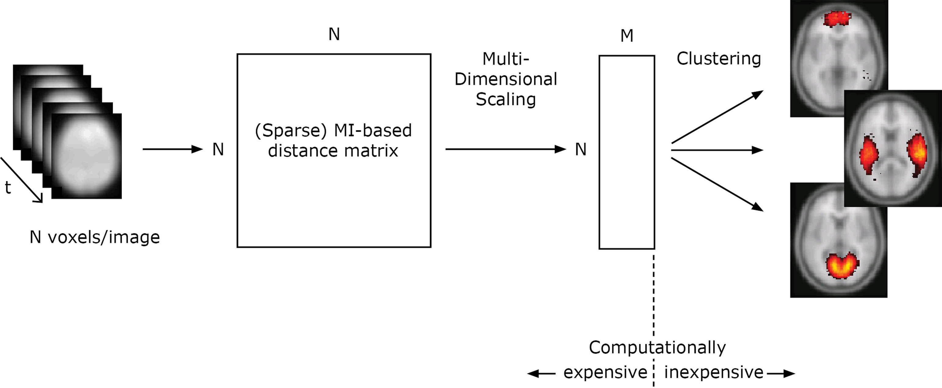
Figure 1. Illustration of the algorithm for one dataset. In this study (Section “Results”), the total number of voxels in each timestep N = 121247 and M was set to 50. The distance matrices from 10 different datasets are combined using an average operation.

Distance matrix

Mutual information is used as a general dependence measure between input voxels i and j,

The values of the voxels are discretized by an interval code. The binning used for the interval code can be determined from a vector quantization run using the values of the dataset (as in Section “Clustering”). This will result in intervals adapted to the data, with more intervals where the distribution of values is dense and fewer where it is sparse.

The probabilities of certain values for a single voxel are estimated from the V image volumes as and . is set as a binary value in the interval k, but it could also have a continuous distribution. For value u_i of voxel i and value u_j of voxel j, p_k is the probability of u_i in the interval k, p_l is the probability of u_j in the interval l and p_kl is the probability of u_i in interval k and u_j in the interval l.

A distance measure in [0,1] is created from the mutual information (Kraskov and Grassberger, 2009) as

, where the joint entropy is used, .

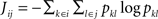The number of bins selected will have an effect on the resolution of the final result as visualized in Figure 2. A representative part of the distance matrix is shown for four different chosen numbers of intervals for the first subject in the dataset described in the Section “Experimental”. The values have been thresholded at a distance of 0.9. A lower number of intervals will result in lower resolution of the distance matrix. The voxels with the strongest relations will still maintain a low distance between each other. A risk in using many bins is that the probabilities in the mutual information calculation are not calculated correctly because the sample size is small. The adaptive bin sizes used should handle this to some degree since it will result in few bins where the sample size is small.

FIGURE 2

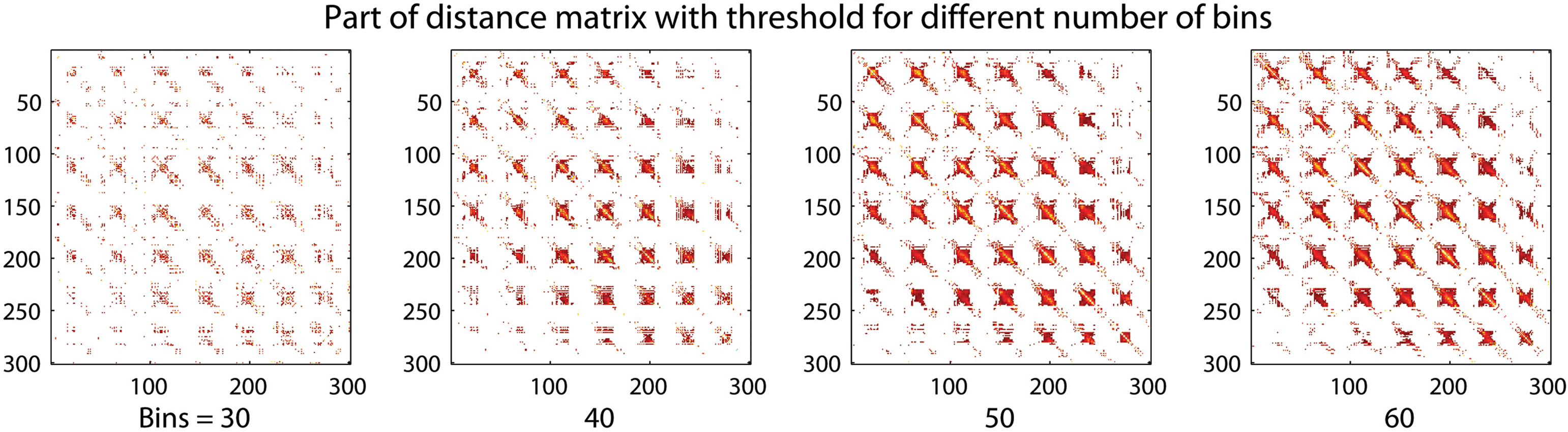
Figure 2. A region of a distance matrix where 30, 40, 50, and 60 discretization intervals, or bins, in the mutual information calculation have been used. The number of bins changes the resolution of the result. A small number of bins still allow the strong relations to be captured.

Multidimensional scaling

The high-dimensional space given by the mutual information over all voxel values is reduced using metric multidimensional scaling (Young, 1985), where the statistical distance relations between the voxels from the distance matrix are used to build up a new, and lower-dimensional space still preserving the distance relations. Here, each voxel is represented by a point, initialized at a random position, and the optimization procedure aims to find a suitable set of positions by iteratively adjusting according to the distance relations by gradient descent until convergence: The difference in a Euclidean distance measure between a pair of voxels in the distance matrix and in their corresponding lower-dimensional space, the stress, was used as a target function to minimize.

Figure 3 shows the average stress for all voxel pairs after convergence for different selections of dimensions for the 60-bin distance matrix from one subject in the previous subsection. A low number of dimensions may have difficulties maintaining the distances in the new space, resulting in a high final stress. If a high enough dimensionality is selected little is gained by adding an additional dimension, seen by the low decrease in stress after 20 dimensions.

FIGURE 3

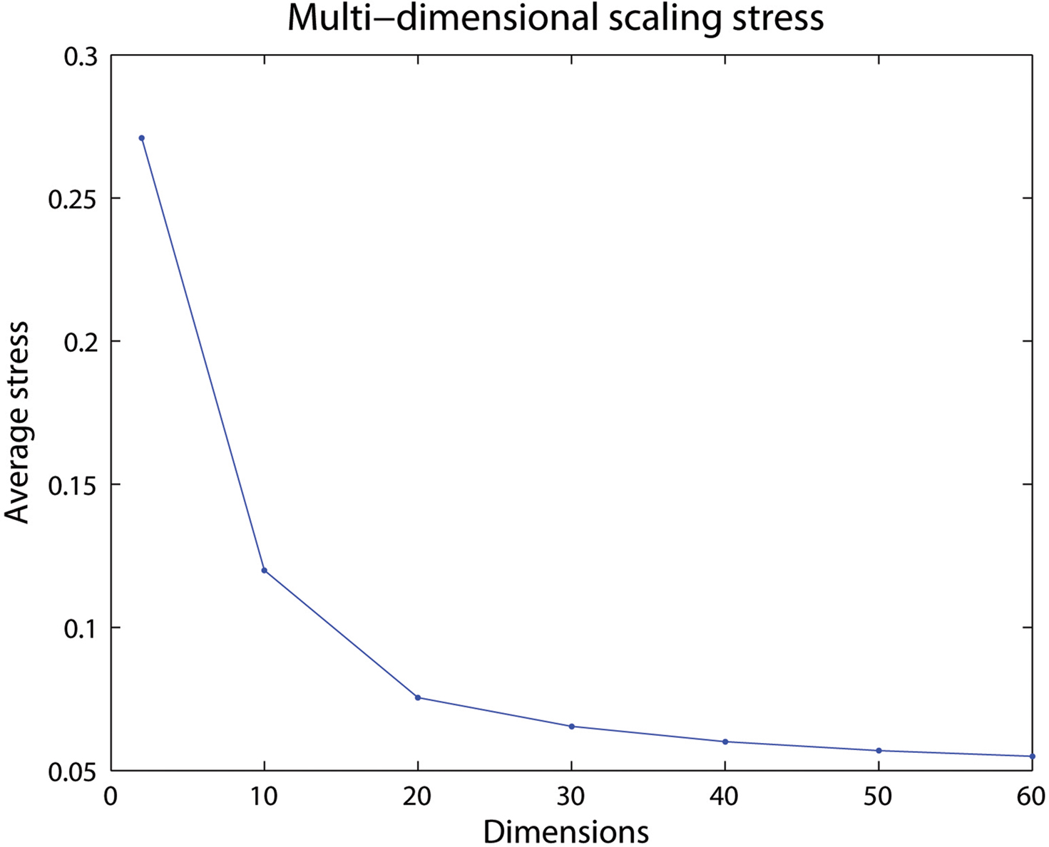
Figure 3. The average stress for different number of dimensions. Here a selected dimensionality over 20 will only give small differences in how well the voxels in the created space are positioned.

Clustering

The voxel positions in the M-dimensional space created from multidimensional scaling reflects the statistical regularities as described by the mutual information. Clustering in this space will join the voxels showing strong statistical dependency as they will have a short distance. We built a parallel implementation of the vector quantization technique competitive selective learning (CSL) (Ueda and Nakano, 1994) both for the clustering into cluster components reflecting the strong statistical regularities and the interval coding division mentioned previously. However, any other clustering algorithm could have been used.

In the same way as traditional competitive learning, CSL uses voxel position x_i to update the position of the closest, by a Euclidean measure, cluster center y by

Here, ε determines the amount of change for the cluster center position in each iteration, and is typically gradually decreased during the training phase. In addition, CSL reinitializes cluster centers in order to avoid local minima using a selection mechanism according to the equidistortion principle (Ueda and Nakano, 1994).

The distortion measure gives an estimate of how well the cluster centers describe the original data. Using Euclidean distances, the distortion from one cluster center can be defined over all data points belonging to cluster center m as

A measure of the average distortion over all C cluster centers in the M-dimensional space, (Ueda and Nakano, 1994), can be used to describe how suitable a given number of clusters are for the data distribution, as seen in the Section “Results”.

Integrating Multiple Datasets

The distance matrix is independent from the value distribution of the original data and the source of the data. Contrary to methods that work with the absolute values, using the relations allows us to combine distance matrices that could be from different datasets or even different data sources. Depending on what we want to evaluate, we can combine the individual distance matrices in various ways. For the multiple subject resting-state data in the Section “Results”, we want to add together the individual results to get a more reliable averaged result. To this end, each distance matrix element was set to the average value over all the individual distance matrices. That is, each dataset was weighted the same. In other applications, where the individual datasets may have different sources, they could be weighted differently. Other operations could also be considered, i.e., a comparison between datasets could be implemented by a subtraction operation between distance matrices.

Experimental

MR Data Acquisition and Data Pre-Processing

Input to the algorithm consisted of 300 MR echo-planar image volumes sensitized to blood oxygenation level dependent (BOLD) signal changes acquired during 10 min of continuous rest (fixating on a cross-hair) in 10 subjects (Fransson, 2006). Functional MR images were acquired on a Signa Horizon Echospeed 1.5 Tesla General Electric MR scanner (FOV = 220 × 220 mm, 64 × 64 matrix size, TR/TE = 2000/40 ms, flip = 80°; number of slices = 29). Further details can be found in a previous paper by Fransson (2006). All images were realigned, normalized to the MNI template within SPM (Statistical Parametrical Mapping, Welcome Trust Center for Neuroimaging, London, Friston et al., 1995) and spatially smoothed with a FWHM = 12 mm. As a final pre-processing step, a rough cropping of the data was performed, for which the non-brain voxels were excluded from further analysis, removing 21% of the data and resulting in a total of 121247 brain voxels.

MR Data Analysis

For each of the 10 resting-state fMRI datasets the original voxel values were interval coded using vector quantization into 60 intervals based on the 1/3 first time steps. Separate distance matrices were calculated for all of the 10 subjects and combined by an average operation, where the mean was taken for each matrix element over all distance matrices. This resulted in a combined distance matrix of dimensions 121247 × 121247. Multidimensional scaling used the distance matrix to create a lower-dimensional map reflecting the statistical relations. In accordance with the discussion in Section “Multidimensional scaling” and Figure 3, the map dimension was set to a number that would clearly be able to maintain the distances in the new space, 50. This gave a total matrix size of 12147 × 50. The clustering algorithm was used to create all possible decompositions between 5 and 115 components. The distance determining which voxels should belong to a group when visualizing the results was specified by a threshold parameter set to 0.4. A voxel can belong to multiple components given the high-dimensional space. For instance, in some dimensions it could be close to one cluster and in others another.

Results

Figure 4 shows the main results from applying the mutual- information based algorithm to the 10 resting-state fMRI datasets for 60 components. Apart from components that showed a very strong spatial resemblance to the patterns typically caused by cardio/respiratory pulsations, susceptibility-movement related effects, subject movements as well as components that were mainly located in cerebro-spinal fluid and white matter areas, 12 components showed connectivity patterns that were located in gray matter. Figures 4A,B show the resting-state networks typically associated with the left and right dorso-lateral parietal-frontal attention network, respectively. Further, Figure 4C shows a bilateral connectivity pattern that encloses the left and right auditory cortex whereas Figure 4D shows a resting-state network that includes the medial and lateral aspects of the sensorimotor cortex. The precuneus/posterior cingulate cortex together with the lateral parietal cortex and a small portion of the medial prefrontal cortex is included in the network shown in Figure 4E. The most anterior part of the medial prefrontal cortex is depicted in Figure 4F. The occipital cortex is by the algorithm divided into three sub-networks that encompasses the anterior/inferior (Figure 4G), posterior (Figure 4H) as well the primary visual cortex (Figure 4K). Figure 4I shows a network that includes the precuneus/posterior cingulate cortex, lateral parietal cortex as well as the medial prefrontal cortex. The network depicted in Figure 4J involves the bilateral temporal pole/insula region. Finally, the cerebellum was included in the network shown in Figure 4L.

FIGURE 4

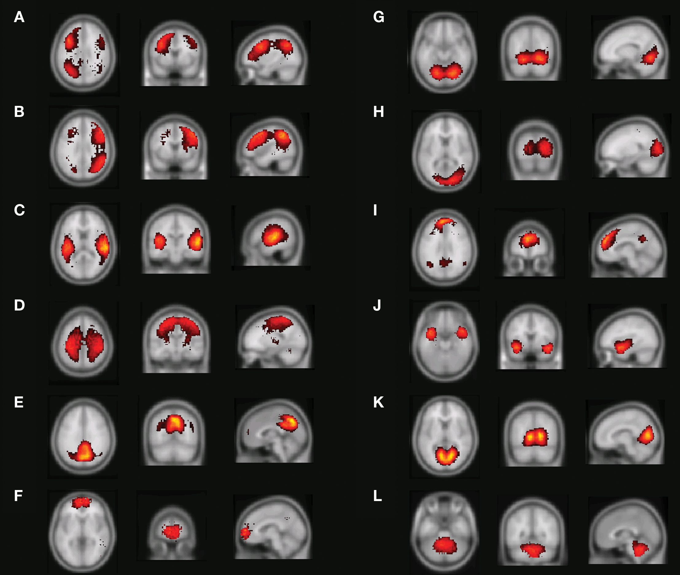
Figure 4. Resting-state networks from a 60-part decomposition: (A, B) Left/right fronto-parietal attention network, (C) primary auditory cortex, (D) lateral and medial sensorimotor cortex, (E) posterior cingulate cortex/precuneus, (F) medial prefrontal cortex, (G) anterior/inferior visual cortex, (H) lateral/posterior visual cortex, (I) default network, (J) temporal pole/insula, (K) primary visual cortex (L), and the cerebellum. The color coding shows how far from the cluster center a given voxel is where brighter red-yellowness indicates a shorter distance to the cluster center.

Networks and Sub-Networks

The distortion derived from the clustering algorithm can be used as a measure of how well various decompositions into resting-state networks suit the data. Figure 5A shows the mean distortion as defined in Section “Clustering” for each network in all decompositions between 5 and 115. The rapid decline for a small number of decompositions tells us that each addition of another cluster will explain the data better. The mean distortion is not changed as much after 30–40 clusters. Additional clustering will result in splitting of the statistically strong networks into their corresponding sub-networks.

FIGURE 5

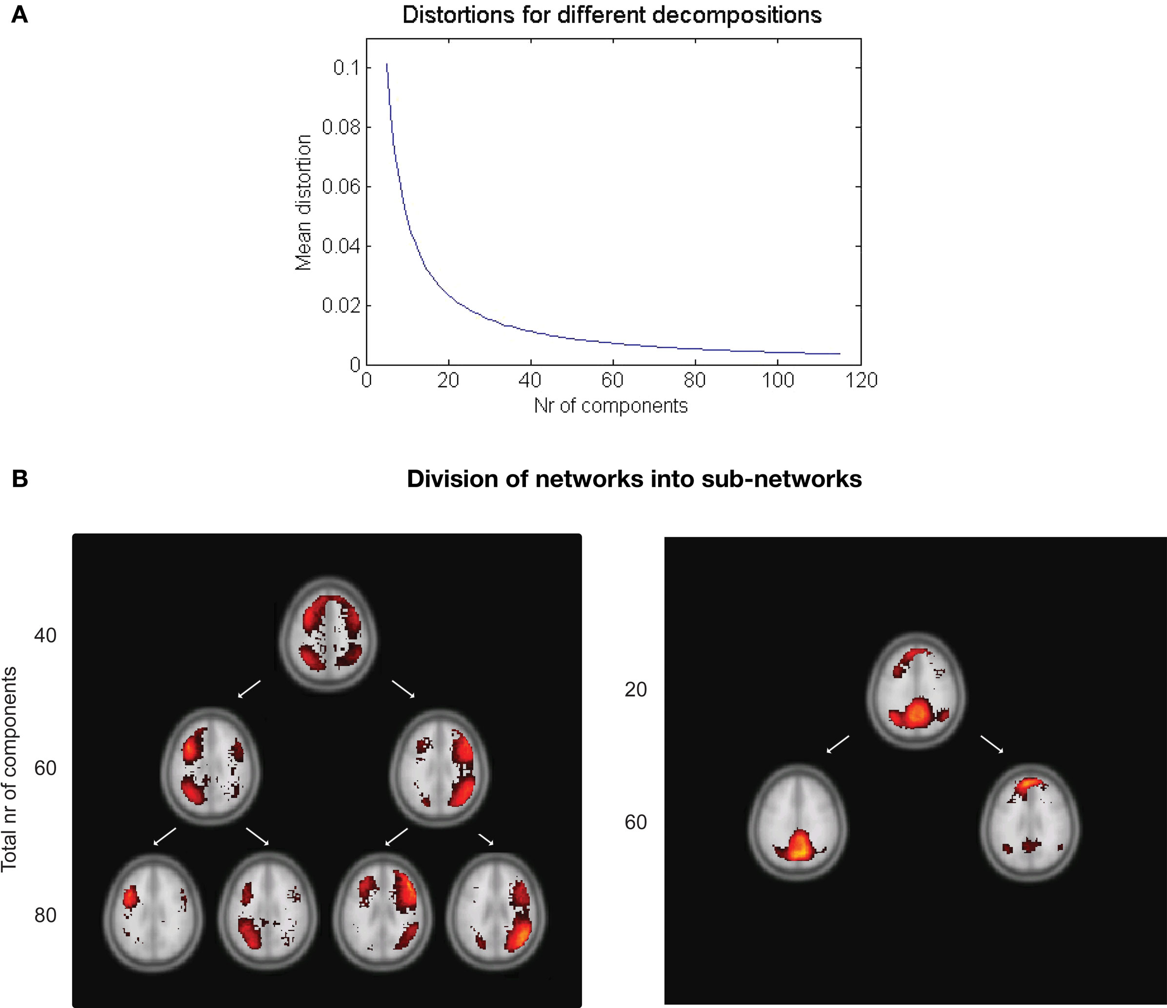
Figure 5. (A) Mean distortion for various decompositions. The distortion measure can be used to predict a suitable number of clusters. (B) Example of the decomposition depending on the total number of clusters chosen. Left: The fronto-parietal attention networks shown in a 40, 60, and 80 decomposition. Right: A splitting of the default network occurs between the 20 and 60 decomposition.

Examples of this can be seen in Figure 5B. The left and right fronto-parietal attention networks are grouped together in the 40 clusters decomposition. At 60 they are separated into their left and right part. Increasing the number of clusters will result in further decomposition into their sub-networks as in the 80 decomposition. A similar splitting is seen for the default network.

Computational Costs

The calculation of the distance matrices is the computationally most expensive operation in the algorithm – when run on the entire dataset it scales with the number of voxels as N² and linearly with the number of time steps and individual datasets. The memory usage can be kept low also on much larger datasets than used here by treating the distance matrix as a sparse matrix in the parallel implementation. The calculation of a distance matrix is trivially parallelizable and involves no expensive communication between the nodes involved in the computation, contrary to parallel implementations of ICA (Keith et al., 2006).

For the resting-state data where the number of voxels was 121247, each distance matrix, one for each subject, took about 30 min to calculate on 512 nodes on a Blue Gene/L machine. However, they could have been run in parallel as each distance matrix is independent from the others. The iterative implementation of multidimensional scaling was run for about 4 h, until convergence. The MDS scales only with the number of voxels and dimensions of the resulting matrix, not with the number of datasets or time steps. These times could most likely be reduced significantly; both by optimizing the code and by considering alternative implementations of the algorithm steps.

The decomposition into different components or clusters is entirely separated from the calculation of the statistics, and since the matrix produced by the MDS is quite small, this is computationally an inexpensive step. All decompositions between 5 and 115 took about 1 h to create on 128 nodes. This is an advantage in certain applications over methods where the number of components to decompose the statistics into has to be manually predetermined. Computationally inexpensive decomposition allows for rapid visualization of the statistics on different spatial scales. Depending on what one is interested in, different decompositions may be of interest.

Discussion

We have described a novel data-driven fMRI cluster analysis method based on multidimensional scaling and mutual information based clustering and shown its applicability for analysis of multi-subject resting-state fMRI data sets. It is relevant to compare the present findings of resting-state networks driven by intrinsic BOLD signal changes during rest with previous investigations that have used other data-driven approaches. The studies of Beckmann et al. (2005), De Luca et al. (2006), and Damoiseaux et al. (2006) as well as the recent study by Smith et al. (2009) all used ICA based approaches to study resting-state functional connectivity, whereas the study by van den Heuvel et al. (2008) used an approach based on a normalized cut graph clustering technique.

On a general level, our results are in good agreement with the findings reported by all four previous investigations. The networks that covered the left and right fronto-parietal cortex (Figures 4A,B) were also detected by all previous investigations, although the left and right network was merged into a single network in the Beckmann et al.’s study (2005) (see also discussion below regarding merging/division of networks and its potential significance). Similarly, the networks that encompassed the auditory cortex (Figure 4C) and the sensorimotor areas (Figure 4D) showed a good spatial congruence with all four previously reported investigations. The network that foremost targeted the primary visual cortex (Figure 4G) shows a large degree of similarity to the networks shown by the De Luca, Damoiseaux, and Smith studies, whereas the primary visual cortex network was merged with the sensorimotor network in the van den Heuvel study (however, an additional explorative analysis revealed separate visual and motor networks, see van den Heuvel et al., 2008 for further information). The network that included the ventro-medial part of prefrontal cortex (Figure 4F) was apparent in all previous studies except the De Luca study. Further, the split of the occipital cortex into a lateral/posterior part (Figure 4H) and an inferior/anterior part (Figure 4G) was also detected by the recent Smith study, but the two networks were merged in a single network in the De Luca study. The network that involves the bilateral temporal pole/insula region (Figure 4J) was similarly detected in the Damoiseaux as well as in the van den Heuvel study. The cerebellar network (Figure 4L) was also found in the Smith study whereas the default mode network (DMN) (Figure 4I) has been reported by all four previous investigations. Finally, the network depicted in Figure 4E that encloses the posterior part of the default network was also found in the van den Heuvel study.

An important aspect of our methodology to cluster the data into resting-state networks and noise-related components is the distortion quantity that provides a measure of how well a specific cluster decomposition fits the data. By examining the degree of distortion as a function of the number of decompositions chosen, information regarding the topological hierarchy of resting-state networks in the brain can be obtained. In the present analysis, this was exemplified for the fronto-parietal network (Figure 5B left) as well as for the default network (Figure 5B right). Regarding the fronto-parietal attention network, previous studies using data-driven methods (De Luca et al., 2006) as well as ROI seed-region based investigations (Fox et al., 2005; Fransson, 2005) have described this collection of brain regions as a single network, whereas other studies have described the collection of the brain regions typically attributed to the fronto-parietal attention network as two separate, lateralized networks that are largely left–right mirrors of each other (Damoiseaux et al., 2006; van den Heuvel et al., 2008; Smith et al., 2009). Indeed, it has previously been noted that the fronto-parietal attention network is often bilaterally activated in tasks that require top–down modulated attention (Corbetta and Shulman, 2002) whereas a unilateral activation is commonly observed for tasks that contain elements of language (left) or pain/perception (right) (Smith et al., 2009). In addition, a recent study has shown that the left side of the fronto-parietal attention network (Figures 4A and 5B) is conjunctively activated by intrinsic, resting-state activity as well as for language related tasks (Lohmann et al., 2009). Taken together, these results speaks to the notion that there are aspects of attention-driven cognitive processes that involve both the left and right parts of the network, and at the same time, a left–right division of cognitive labor exist at a sublevel within the same network.

In a similar vein, we observed a putative division of the DMN into an anterior and posterior sub-network (Figures 4E,I), respectively. Similar to the division of the fronto-parietal network, the spatial separation of the DMN was not complete. A small degree of activity of the posterior part, e.g., the precuneus/PCC, is present in the anterior sub-default network (Figure 4I) and vice versa for the medial prefrontal cortex in the posterior sub-default network (Figure 4E). Our finding of a potential anterior/posterior topographical hierarchy are in line with previous reports that have suggested that the precuneus/PCC region constitute a network hub in the DMN (Buckner et al., 2008; Fransson and Marrelec, 2008) as well as the MPFC (Buckner et al., 2008). The cognitive interpretation of a putative anterior/posterior division of the DMN is at present not clear. Speculatively, the split of the DMN observed here could reflect the fact that the anterior sub-network of the DMN, including a hub in the MPFC, is tentatively preferentially more involved in the self-referential aspects of mental processing (Gusnard et al., 2001), whereas the posterior part in which the precuneus/PCC region acts as a hub is oriented towards tasks that contains elements of retrieval of episodic memory and recognition (Dörfel et al., 2009).

The method could be extended in various ways. The MDS step could be extended to better conserve non-linear relationships as in the Isomap algorithm (Tenenbaum et al., 2000). More explicit hierarchical clustering algorithms may be used to further characterize the statistical relationships between clusters of different spatial scales (Meunier et al., 2009). The resulting MDS matrix could also be studied by other means than clustering algorithms, such as using PCA. Measurements other than mutual information could be used to study other aspects of the data, such as causal relations as determined by Granger causality (Roebroeck et al., 2005). A change of statistical expression to evaluate would generally involve no more changes than replacing the calculation determining an element value in the distance matrix. The method described here was partly based on a cortical information processing model (Lansner et al., 2009) which also included a classification step. Incorporating classification as a final step in the method would make it a good candidate for applications such as “brain reading” (Eger et al., 2009).

Conclusion

The generic method proposed brings a number of new properties to a model-free analysis of fMRI data: The separation of the computationally demanding calculation of the statistics and the decomposition step, which is computationally inexpensive, allows for rapid visualization and exploration of the statistics on multiple spatial scales. Input data can be handled independently and weighted together in various ways depending on the application, both for data from different subjects and data from different sources. The algorithm has been implemented completely in parallel code; this means that we can calculate the statistics over all of the input data, without any dimensionality reduction, which allows for whole-brain analysis on a voxel level. It can handle datasets with large input sizes as well as large collections of datasets in databases. Some of its properties for exploratory data analysis and its applicability to fMRI have been demonstrated on resting-state data and shown to be in agreement with findings from studies using other methods.

Our method is generic and does not use any specific properties of fMRI data. It may therefore also be applicable to completely different kinds of data. We are currently exploring its use in, e.g., PET data analysis. It further remains to optimize the method, possibly taking advantage of GPU implementation of certain steps in the algorithm.

Conflict of Interest Statement

The authors declare that the research was conducted in the absence of any commercial or financial relationships that could be construed as a potential conflict of interest.

Acknowledgments

This work was partly supported by grants from the Swedish Science Council (Vetenskapsrådet, VR-621-2004-3807; www.vr.se), the European Union (FACETS project, FP6-2004-IST-FETPI-015879; http://facets.kip.uni-heidelberg.de) and the Swedish Foundation for Strategic Research (through the Stockholm Brain Institute; www.stockholmbrain.se).

References

Beckmann, C. F., DeLuca, M., Devlin, J. T., and Smith, S. M. (2005). Investigations into resting-state connectivity using independent component analysis. Philos. Trans. R. Soc. Lond., B, Biol. Sci. 360, 1001–1013.

Pubmed Abstract | Pubmed Full Text | CrossRef Full Text

Buckner, R. L., Andrews-Hanna, J. R. , and Schacter, D. L. (2008). The brain’s default network: anatomy, function and relevance to disease. Ann. N Y Acad. Sci. 1, 1124–1138.

Chuang, K. H., Chiu, M. J., Lin, C. C., and Chen, J. H. (1999). Model-free functional MRI analysis using Kohonen clustering neural network and fuzzy C-means. IEEE Trans. Med. Imaging 18, 1117–1128.

Pubmed Abstract | Pubmed Full Text | CrossRef Full Text

Corbetta, M., and Shulman, G. M. (2002). Control of goal-driven and stimulus-driven attention in the brain. Nat. Rev. Neurosci. 3, 201–215.

Pubmed Abstract | Pubmed Full Text | CrossRef Full Text

Damoiseaux, J. S., Rombouts, S. A. R. B., Barkhof, F., Scheltens, P., Stam, C. J., Smith, S. M., and Beckmann, C. F. (2006). Consistent resting-state networks across healthy subjects. Proc. Natl. Acad. Sci. U.S.A. 103, 13848–13853.

Pubmed Abstract | Pubmed Full Text | CrossRef Full Text

De Luca, M., Beckmann, C. F., De Stefano, N., Matthews, P. M., and Smith, S. M. (2006). fMRI resting-state networks define modes of long-distance interactions in the human brain. Neuroimage 29, 1359–1367.

Pubmed Abstract | Pubmed Full Text | CrossRef Full Text

Dörfel, D., Werner, A., Schaefer, M., von Kummer, R., and Karl, A. (2009). Distinct brain networks in recognition memory share a defined region in the precuneus. Eur. J. Neurosci. 30, 1947–1959.

Pubmed Abstract | Pubmed Full Text | CrossRef Full Text

Eger, E., Michel, V., Thirion, B., Amadon, A., Dehaene, S., and Kleinschmidt, A. (2009). Deciphering cortical number coding from human brain activity patterns. Curr. Biol. 19, 1608–1615.

Pubmed Abstract | Pubmed Full Text | CrossRef Full Text

Fox, M. D., Snyder, A. Z., Vincent, J. L., Corbetta, M., Van Essen, D. C., and Raichle, M. E. (2005). The human brain is intrinsically organized into dynamic, anticorrelated functional networks. Proc. Natl. Acad. Sci. U.S.A. 102, 9673–9678.

Pubmed Abstract | Pubmed Full Text | CrossRef Full Text

Fransson, P. (2005). Spontaneous low-frequency BOLD signal fluctuations – an fMRI investigation of the resting-state default mode of brain function hypothesis. Hum. Brain Mapp. 26, 15–29.

Pubmed Abstract | Pubmed Full Text | CrossRef Full Text

Fransson, P. (2006). How default is the default mode of brain function? Further evidence from intrinsic BOLD fluctuations. Neuropsychologia 44, 2836–2845.

Pubmed Abstract | Pubmed Full Text | CrossRef Full Text

Fransson, P., and Marrelec, G. (2008). The precuneus/posterior cingulate cortex plays a pivotal role in the default network. Evidence from a partial correlation network analysis. Neuroimage 42, 1178–1184.

Pubmed Abstract | Pubmed Full Text | CrossRef Full Text

Friston, K. J., Holmes, A. P., Worsley, K. J., Poline, J. P., Frith, C. D., and Frackowiak, R. S. J. (1995). Statistical parametric maps in functional imaging: a general linear approach. Hum. Brain Mapp. 2, 189–210.

CrossRef Full Text

Gusnard, D. A., Akbudak, E., Shulman, G. L., and Raichle, M. E. (2001). Medial prefrontal cortex and self-referential mental activity: relation to a default mode of brain function. Proc. Natl. Acad. Sci. U.S.A. 98, 4259–4264.

Pubmed Abstract | Pubmed Full Text | CrossRef Full Text

Golland, Y., Golland, P., Bentin, S., and Malach, R. (2008). Data-driven clustering reveals a fundamental subdivision of the human cortex into two global systems. Neuropsychologia 46, 540–553.

Pubmed Abstract | Pubmed Full Text | CrossRef Full Text

Hinrichs, H., Heinze, H. J., and Schoenfeld, M. A. (2006). Causal visual interactions as revealed by an information theoretic measure and fMRI. Neuroimage 31, 1051–1060.

Pubmed Abstract | Pubmed Full Text | CrossRef Full Text

Keith, D. B. Hoge, C. C. Frank, R. M., and Malony, A. D. (2006). Parallel ICA methods for EEG neuroimaging. Parallel and Distributed Processing Symposium, 10–20.

Kraskov, A., and Grassberger, P. (2009). MIC: mutual information based hierarchical clustering. Inform. Theory Stat. Learn. 101–123.

Lansner, A., Benjaminsson, S., and Johansson, C. (2009). “From ANN to biomimetic information processing,” in Studies in Computational Intelligence 188, eds A. Gutierrez and S. Marco. (Heidelberg: Springer Berlin), 33–43.

Lohmann, G., Hoehl, S., Brauer, J., Danielmeier, C., Bornkessel-Schlesewsky, I., Bahlmann, J., Turner, R., and Friederici, A. (2009). Setting the frame: the human brain activates a basic low-frequency network for language processing. Cereb. Cortex, PMID 19783579.

McKeown, M. J., Makeig, S., Brown, G. G., Jung, T.-P., Kindermann, S. S., Bell, A. J., and Sejnowski, T. J. (1998). Analysis of fMRI data by blind separation into independent spatial components. Hum. Brain Mapp. 6, 160–188.

Pubmed Abstract | Pubmed Full Text | CrossRef Full Text

Meunier, D., Lambiotte, R., Fornito, A., Ersche, K., and Bullmore, E. T. (2009). Hierarchical modularity in human brain functional networks. Front. Neuroinform. 3, 37. doi:10.3389/neuro.11.037.2009.

CrossRef Full Text

Mezer, A., Yovel, Y., Pasternak, O., Gorfine, T., and Assaf, Y. (2009). Cluster analysis of resting-state fMRI time series. Neuroimage 45, 1117–1125.

Pubmed Abstract | Pubmed Full Text | CrossRef Full Text

Roebroeck, A., Formisano, E., and Goebel, R. (2005). Mapping directed influence over the brain using granger causality and fMRI. Neuroimage 25, 230–242.

Pubmed Abstract | Pubmed Full Text | CrossRef Full Text

Salvador, R., Martínez, A., Pomarol-Clotet, E., Sarró, S., Suckling, J., and Bullmore, E. (2007). Frequency based mutual information measures between clusters of brain regions in functional magnetic resonance imaging. Neuroimage 35, 83–88.

Pubmed Abstract | Pubmed Full Text | CrossRef Full Text

Salvador, R., Suckling, J., Coleman, M. R., Pickard, J. D., Menon, D., and Bullmore, E. (2005). Neurophysiological architecture of functional magnetic resonance images of human brain. Cereb. Cortex 15, 1332–1342.

Pubmed Abstract | Pubmed Full Text | CrossRef Full Text

Smith, S. M., Fox, P. T., Miller, K. L., Glahn, D. C., Fox, P. M., Mackay, C. E., Filippini, N., Watkins, K. E., Toro, R., Laird, A. R., and Beckmann, C. F. (2009). Correspondence of the brain’s functional architecture during activation and rest. Proc. Natl. Acad. Sci. U.S.A. 106, 13040–13045.

Pubmed Abstract | Pubmed Full Text | CrossRef Full Text

Smith, S. M., Jenkinson, M., Woolrich, M., Beckmann, C., Behrens, T., Johansenberg, H., Bannister, P., DeLuca, M., Drobnjak, I., and Flitney, D. (2004). Advances in functional and structural MR image analysis and implementation as FSL. Neuroimage 23, 208–219.

CrossRef Full Text

Tenenbaum, J. B., Silva, V., and Langford, J. C. (2000). A global geometric framework for nonlinear dimensionality reduction. Science 290, 2319–2323.

Pubmed Abstract | Pubmed Full Text | CrossRef Full Text

Ueda, N., and Nakano, R. (1994). A new competitive learning approach based on an equidistortion principle for designing optimal vector quantizers. Neural Networks 7, 1211–1227.

CrossRef Full Text

van den Heuvel, M., Mandl, R., and Hulshoff Pol, H. (2008). Normalized cut group clustering of resting-state fMRI data. PLoS One 3, e2001. doi:10.1371/journal.pone.0002001.

Pubmed Abstract | Pubmed Full Text | CrossRef Full Text

Young, F. W. (1985). “Multidimensional scaling,” in Encyclopedia of Statistical Sciences, Vol. 5, eds S. Kotz, N. L. Johnson, and C. B. Read (New York, NY: Wiley), 649–659.