Fourier-transforming with quantum annealers

1. Introduction

The birth of Quantum Computation may be traced back to the seminal papers of Feynman [1] and Deutsch [2] in the 1980's. However, it was Peter Shor in 1994 who rekindled the interest in the field among both scientists and the general public, by devising an efficient algorithm for factoring large integers [3]. This discovery by Shor was exciting for two main reasons. First, because it was the first complete (i.e., non-blackbox) algorithm to show that quantum algorithms may in principle be exponentially faster than their classical counterparts, and second, because of the practical significance of the algorithm, namely, undermining the security of one of the most widely used cryptographic protocols, the RSA [4].

Despite intensive efforts, the actual implementation of Shor's algorithm in an experimental setup is, almost 20 years after its inception, very limited. This is due to the multitude of technological challenges that quantum-computer engineers and experimentalists are still facing, the most prominent being the control or removal of quantum decoherence [5]. Since the first demonstration of Shor's algorithm in 2001 at IBM, factoring the number 15 using an NMR implementation of a quantum computer with 7 qubits [6], Shor's algorithm has been demonstrated by several other groups that have implemented the algorithm using photonic qubits [7, 8]. However, the most recent attempt in 2012 which also set the record for largest number factorized by Shor's algorithm, successfully factorized only 21 [9], where even these limited achievements have been recently contested by arguments that factoring small numbers quantum-mechanically for which the answer is known in advance extremely oversimplifies the procedure [10].

Recent promising experimental research findings [11–13], as well as intensive theoretical work [see, e.g., 14–23] in the field of Adiabatic Quantum Computing (AQC) suggest the possibility that some of the experimental difficulties may be overcome by the use of “quantum annealing” devices, which implement the simple yet potentially-powerful quantum-adiabatic algorithmic approach proposed by Farhi et al. [24] about a decade ago. AQC is an analog, continuous, quantum computing paradigm, and as such it has the potential of being easier to implement successfully, offering several advantages over the “traditional” gate model, in the form of inherent fault-tolerance and natural robustness against decoherence and dephasing [25, 26].

These aforementioned findings have generated a great deal of theoretical and experimental research set out to explore the practical capabilities, as well as the limitations, of quantum annealers. One of the most interesting questions raised in this regard, was naturally, the possibility of implementing hugely-practical and powerful algorithms such as Shor's integer factorization on a quantum adiabatic device. However, despite numerous efforts [see, e.g., 27, 28], an efficient quantum-adiabatic analog to Shor's algorithm has not been found to date. This is despite recent studies [29–32] suggesting that the equivalence between AQC and the gate model is even stronger than the one implied by the principles of polynomial equivalence prescribed in the seminal study of Aharonov et al. [33].

A recent work that examined the theoretical feasibility of an optimally-constructed adiabatic algorithm for Simon's problem [34], which shares many similarities with, and in fact provided the motivation for, Shor's algorithm, has introduced a somewhat-novel approach for constructing quantum adiabatic algorithms [32]. Within this approach, which will be discussed in more detail next, a multitude of adiabatic evolutions is executed simultaneously in parallel and a single measurement at the end of the run, performed on the entire system, is used to extract valuable information.

Here, we shall attempt to generalize the above approach in order to construct an algorithm for the “quantum component” of Shor's algorithm, namely the Quantum Fourier Transform (QFT). As we shall see, the QFT algorithm, used in Shor's integer factorization routine to detect the periodicity of a cyclic function, may be constructed quantum-adiabatically very similarly to the way it is implemented in the gate model, namely broken into “building blocks” each operating on a small number of qubits at a time. This construction of adiabatic QFT can then be used to adiabatically implement Shor's integer factorization algorithm as well as other important quantum algorithms, such as the quantum phase estimation algorithm for estimating the eigenvalues of a unitary operator, and algorithms for the hidden subgroup problem [see, e.g., 35] for more details.

As we shall see, the approach taken here to convert the QFT circuit to adiabatic processes differs in several important aspects from existing protocols designed to efficiently translate gate-model circuits into quantum adiabatic algorithms, such as history state-based constructions [33], ground-state quantum computation approaches [36] or other schemes [37]. Moreover, the adiabatic procedure that emerges from the procedure suggested here, will turn out to fundamentally differ from traditional AQC evolutions. These matters will be discussed in some detail in the concluding section.

In the following, we first briefly discuss the main principles of AQC in order to demonstrate the idea behind this paradigm of computing and to establish notation. We move on to consider in some detail the QFT algorithm and the gates used there, and then describe how these may be constructed via adiabatic evolutions to form an adiabatic QFT algorithm. Finally, we conclude with some comments about the experimental feasibility of the algorithm, and its relations to the gate model and traditional AQC.

2. Principles of Adiabatic Quantum Computing

In AQC, one normally (albeit not exclusively) seeks the minimum value and corresponding input configuration of a given cost function, that is encoded as a final (or “problem”) Hamiltonian, $\widehat{H}$_f, such that the ground state of the final Hamiltonian and its energy are the solution to the original problem [38]. To find the solution, the system is prepared in the ground state of another “beginning” (or “driver”) Hamiltonian $\widehat{H}$_b that must not commute with $\widehat{H}$_f and has a ground state that is fairly easy to prepare. The Hamiltonian of the system is then slowly interpolated between $\widehat{H}$_b and $\widehat{H}$_f, normally by an interpolation of the form $\widehat{H}$(t) = f₁(t) $\widehat{H}$_b + f₂(t) $\widehat{H}$_f where f₁(t) [f₂(t)] is a smoothly-varying function of time that is positive (zero) at t = 0 and zero (positive) at t = . Here, stands for the runtime of the algorithm. If this process is done slowly enough, the system will stay close to the ground state of the instantaneous Hamiltonian throughout the evolution [39, 40], so that one finally obtains a state close to the ground state of $\widehat{H}$_f. At this point, measuring the state will give the solution of the original problem with high probability.

It is clear from the above description, that the analog, continuous, nature of AQC is inherently very different form the discrete nature of gate model algorithms within which unitary operations act sequentially to advance the state of the system. For this reason it has been hard so far to draw meaningful analogies between AQC and the gate model. Nonetheless, in what follows, we shall show how one could utilize the above principles to construct the necessary “building blocks” or “adiabatic gates” for the construction of an adiabatic QFT algorithm, analogously to the manner in which the unitary gates of the gate model are used to construct circuits. We begin by describing the QFT algorithm.

3. The QFT Algorithm

QFT is a linear transformation on quantum bits, and is the quantum analog of the classical discrete Fourier transform (DFT) [41] applied to the vector of amplitudes of a quantum state. The classical Fourier transform acts on a vector of complex numbers (x₀, …, x_N−1) and maps it to another (y₀, …, y_N−1) according to

$\begin{array}{cc}{y}_k=\frac{1}{\sqrt{N}}{\displaystyle \sum _{j=0}^{N-1}{x}_j}{\omega }^{jk},& (1)\end{array}$

where $\omega ={\text{e}}^{\frac{2\pi i}{N}}$ is a primitive N-th root of unity. Similarly, the quantum Fourier transform acts on a quantum state ${\displaystyle {\sum }_{i=0}^{N-1}{x}_i|i\rangle }$ and maps it to a quantum state ${\displaystyle {\sum }_{i=0}^{N-1}{y}_i}|i\rangle$ via the above mapping.

Shor [3] was the first to show that using a simple decomposition, the discrete Fourier transform can be implemented as a quantum circuit consisting of only O(n²) Hadamard, controlled-phase shift and SWAP gates, each being efficiently implementable, where n is the number of qubits [35]. The remarkable feature of Shor's quantum circuit was that the classical analog of the algorithm, the DFT, is known to be exponentially-slower and takes O(n 2ⁿ) basic (classical) operations. It is important to note however, that while the classical discrete Fourier transform outputs a vector whose components are all fully accessible at the end of the algorithm, in the quantum case, the outcome of QFT is a quantum state, the amplitudes of which are only very partially accessible by quantum measurements. The circuit for QFT is given in Figure 1 for the reader's convenience [for more details, see, e.g., 35].

FIGURE 1

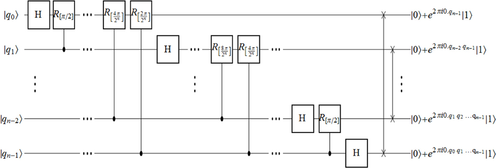
Figure 1. Implementation of the QFT circuit [for more details, see, e.g., 35] using Hadamard, controlled-phase-shift and SWAP gates.

In what follows, we show that the Hadamard, controlled-phase-shift and SWAP gates may also be implemented using only adiabatic evolutions. To that aim, we shall describe several quantum adiabatic algorithms that we shall argue may be used to mimic the outcome of the above gates, and by doing so allow for the construction of an equivalent “adiabatic circuit” for QFT that may be constructed similarly to the way it is constructed in the gate model. We shall begin by describing the adiabatic Hadamard gate and then move on to describe the slightly more complicated controlled-phase-shift and SWAP gates.

3.1. Adiabatic Hadamard

The Hadamard gate is a single-qubit gate that acts on the states of the computational basis in the following way: |0〉 ↦ |+_x〉 and |1〉 ↦ |−_x〉. Here, |0〉 and |1〉 stand for the two computational-basis states, which we shall identify as spins pointing in the positive and negative z-directions, respectively, and |±_x〉 are the corresponding x-basis states.

To apply a Hadamard gate quantum-adiabatically, consider now a single qubit (that may or may not be a part of a larger system of qubits) in an arbitrary unknown state |ψ〉 = α|0〉 + β|1〉. Let us now attach to it an auxiliary qubit, initialized to the computational |0〉 state:

$\begin{array}{cc}|{\psi }_{\text{b}}\rangle =\left(\alpha |0\rangle +\beta |1\rangle \right)\otimes |0\rangle .& (2)\end{array}$

This will be the initial (or “beginning”) state of an adiabatic algorithm whose evolution will be governed by the two-local Hamiltonian:

$\begin{array}{cc}\widehat{H}(t)=|{+}_y\rangle \langle {+}_y|\otimes {\widehat{H}}_x(t)+|{-}_y\rangle \langle {-}_y|\otimes {\widehat{H}}_{-y}(t),& (3)\end{array}$

where |±_y〉 are the y-basis states and $\widehat{H}$_x(t) and $\widehat{H}$_−y(t) are adiabatic-evolution Hamiltonians that act only within the respective subspaces of the y-axis basis states of the first qubit, projected by the orthogonal projections |±_y〉〈±_y| = 1/2(1 ± σ_y). The adiabatic-evolution Hamiltonians are given by:

$\begin{array}{cc}{\widehat{H}}_x(t)=-\cos \theta (t){\sigma }_z-\sin \theta (t){\sigma }_x& (4)\end{array}$

$\begin{array}{cc}{\widehat{H}}_{-y}(t)=-\cos \theta (t){\sigma }_z+\sin \theta (t){\sigma }_y.& (5)\end{array}$

The time-dependence of these Hamiltonians is given by the angle θ(t) such that θ(t = 0) = 0 and θ(t = ) = θ_f where θ_f is the value of the polar angle θ at the end of the evolution. For simplicity, we shall henceforth assume the dependence θ(t) = θ_ft/, although it should be noted that the precise time dependence of the polar angle θ does not have to be linear. Note that the gaps of the above one-qubit Hamiltonians are constant throughout the evolution and equal to 2.

As can be immediately read off the expressions above, in the course of the adiabatic evolution, the Hamiltonians $\widehat{H}$_x(t) and $\widehat{H}$_−y(t) will act inside two complementary subspaces spanned by |±_y〉, evolving the auxiliary qubit, initially at $|G{S}_x\rangle =\left(\cos \frac{{\theta }_{\text{f}}}{2}|0\rangle +\sin \frac{{\theta }_{\text{f}}}{2}|1\rangle \right)$ [the latter being the ground state of $\widehat{H}$_x()] in the subspace projected by |+_y〉〈+_y| and to $|G{S}_{-y}\rangle =\left(\cos \frac{{\theta }_{\text{f}}}{2}|0\rangle -i\sin \frac{{\theta }_{\text{f}}}{2}|1\rangle \right)$ in the subspace projected by |−_y〉〈−_y|. The trajectories of the auxiliary qubit in the two subspaces on the surface of the Bloch sphere are depicted in Figure 2 for the convenience of the reader. Rewriting the input qubit in terms of the y-basis states, the initial state is

$\begin{array}{cc}|{\psi }_{\text{b}}\rangle =\left(\frac{\alpha -i\beta }{\sqrt{2}}|{+}_y\rangle +\frac{\alpha +i\beta }{\sqrt{2}}|{-}_y\rangle \right)\otimes |0\rangle .& (6)\end{array}$

FIGURE 2

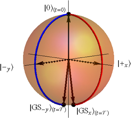
Figure 2. (Color online) adiabatic evolution trajectories of the auxiliary qubit on the surface of the Bloch sphere in the adiabatic Hadamard gate. Starting at the |0〉 state, the state of the qubit “splits” into two trajectories. In the first, it adiabatically evolves from the |0〉 state (north pole) toward the |1〉 (south pole) passing through |+_x〉, maintaining the azimuthal angle of ϕ = 0 (blue dots). The second path passes through |−_y〉 (red dots) with ϕ = 3π/2 throughout the evolution. The final states of the two paths, namely, |GS_x〉 and |GS_−y〉 are described in the text.

The adiabatic procedure will evolve the system into the final state:

$\begin{array}{cc}\begin{array}{l}|{\psi }_{\text{f}}\rangle =\frac{\alpha -i\beta }{\sqrt{2}}|{+}_y\rangle \otimes \left(\cos \frac{{\theta }_{\text{f}}}{2}|0\rangle +\sin \frac{{\theta }_{\text{f}}}{2}|1\rangle \right)\\ +\frac{\alpha +i\beta }{\sqrt{2}}|{-}_y\rangle \otimes \left(\cos \frac{{\theta }_{\text{f}}}{2}|0\rangle -i\sin \frac{{\theta }_{\text{f}}}{2}|1\rangle \right)\\ =\cos \frac{{\theta }_{\text{f}}}{2}\left(\frac{\alpha -i\beta }{\sqrt{2}}|{+}_y\rangle +\frac{\alpha +i\beta }{\sqrt{2}}|{-}_y\rangle \right)\otimes |0\rangle \\ +\sin \frac{{\theta }_{\text{f}}}{2}\left(\frac{\alpha -i\beta }{\sqrt{2}}|{+}_y\rangle -i\frac{\alpha +i\beta }{\sqrt{2}}|{-}_y\rangle \right)\otimes |1\rangle .\end{array}& (7)\end{array}$

which can also be rewritten (neglecting the immaterial global phase) as:

$\begin{array}{cc}\begin{array}{l}|{\psi }_{\text{f}}\rangle =\cos \frac{{\theta }_{\text{f}}}{2}\left(\alpha |0\rangle +\beta |1\rangle \right)\otimes |0\rangle \\ -\sin \frac{{\theta }_{\text{f}}}{2}\left(\frac{\alpha +\beta }{\sqrt{2}}|0\rangle +\frac{\alpha -\beta }{\sqrt{2}}|1\rangle \right)\otimes |1\rangle .\end{array}& (8)\end{array}$

The above expression reveals that a choice of a final polar angle of θ_f = π would yield, with certainty, a final state that is a product of a Hadamard-transformed first qubit and a flipped auxiliary qubit.

It is crucially important to notice that the above adiabatic evolution introduces no relative phase between the two paths, passing through |+_x〉 and |−_y〉, respectively. This can be directly inferred from the symmetries of the Hamiltonian (and can also be deduced by examining the two trajectories described in Figure 2). That there is no relative phase between the two paths is significant for the amplitude-interference in the resultant final states at the end of the process [cf. Equation (8)]. It is therefore important to note at this point that in practical experimental setups, interactions of the system with the environment will generally act to destroy this coherence between the two final states, forcing the time scale of the adiabatic evolution to be significantly shorter than the typical decoherence time of the system-environment interactions.

We have so far shown how a Hadamard gate may be applied quantum-adiabatically without the use of actual conventional gates. The same principles introduced above can be utilized to construct the slightly more complicated controlled-phase-shift and SWAP adiabatic gates.

3.2. Adiabatic Controlled-Phase-Shift Gate

The above scheme may now be modified to apply a controlled-phase-shift gate adiabatically. The controlled-phase-shift gate, depending on the state of the control qubit, will either leave the target qubit unchanged or will execute the transformation (α|0〉 + β|1〉) ↦ (α|0〉 + βe^iϕ|1〉). The adiabatic implementation of the gate is as follows. Our system initially contains two input qubits, the first of which shall be regarded as a control qubit: |ψ〉 = α|00〉 + β|01〉 + γ|10〉 + δ|11〉. An adiabatic controlled-phase-shift is obtained by attaching, as before, an auxiliary qubit to the initial state:

$\begin{array}{cc}|{\psi }_{\text{b}}\rangle =\left(\alpha |00\rangle +\beta |01\rangle +\gamma |10\rangle +\delta |11\rangle \right)\otimes |0\rangle ,& (9)\end{array}$

and constructing the slightly more complicated (in this case, three-local) Hamiltonian:

$\begin{array}{cc}\begin{array}{l}\widehat{H}(t)=|0\rangle \langle |0|\otimes 1\otimes {\widehat{H}}_x(t)\\ +|1\rangle \langle 1|\otimes \left(|0\rangle \langle 0|\otimes {\widehat{H}}_x(t)+|1\rangle \langle 1|\otimes {\widehat{H}}_{\varphi }(t)\right)\end{array}& (10)\end{array}$

where $\widehat{H}$_x(t) is as before and $\widehat{H}$_ϕ(t) = −cos θ(t) σ_z − sin θ(t) (cos ϕσ_x + sin ϕσ_y) whose ground state is $|{+}_{\varphi }\rangle =\frac{1}{\sqrt{2}}\left(|0\rangle +e^{i\varphi }|1\rangle \right)$.

The above Hamiltonian, Equation (10), should be interpreted in the following way. If the control qubit is in the |0〉 state then the auxiliary qubit will evolve according to $\widehat{H}$_x(t) independently of the state of the second qubit. Conversely, if the control qubit is in the |1〉 state, the auxiliary qubit will evolve according to $\widehat{H}$_x(t) when projected onto the |0〉〈0| subspace of the second qubit and according to $\widehat{H}$_ϕ(t) when projected onto the |1〉〈1| subspace.

Choosing, as before, the final polar angle to be θ_f = π, the auxiliary qubit during the application of the above adiabatic Hamiltonian will follow, depending on the state of the first two qubits, either the path [|0〉 ↦ |+_x〉 ↦ |1〉] or [|0〉 ↦ |+_ϕ〉 ↦ |1〉] on the surface of the Bloch sphere. Since the two traversed paths are taken at different azimuthal angles, the final states will differ by a relative phase of ϕ, yielding

$\begin{array}{cc}|{\psi }_{\text{f}}\rangle =\left(\alpha |00\rangle +\beta |01\rangle +\gamma |10\rangle +\delta {\text{e}}^{i\varphi }|11\rangle \right)\otimes |1\rangle ,& (11)\end{array}$

i.e., the final state of the first two qubits will be the desired controlled-phase-shifted state with the auxiliary qubit flipped, as before.

3.3. Adiabatic SWAP Gate

The QFT algorithm uses mainly the Hadamard and controlled-phase-shift gates discussed above (see Figure 1). However, at the end of the QFT, the qubits of the Fourier-transformed state appear in reverse order. To rectify that, the qubits can be swapped using a SWAP gate, which is a two qubit gate that swaps |01〉 ↔ |10〉 and leaves |00〉 and |11〉 unchanged. It is easy to show that SWAP can be accomplished by three controlled-NOT operations where the role of the control qubit switches place at each step [42].

Let us now show how a controlled-NOT gate can be adiabatically accomplished in much the same way as the other two adiabatic gates introduced thus far. Consider now the action of the total Hamiltonian:

$\begin{array}{cc}\begin{array}{l}\widehat{H}(t)=|0\rangle \langle 0|\otimes 1\otimes {\widehat{H}}_x(t)\\ +|1\rangle \langle 1|\otimes \left(|{+}_x\rangle \langle {+}_x|\otimes {\widehat{H}}_x(t)+|{-}_x\rangle \langle {-}_x|\otimes {\widehat{H}}_{-x}(t)\right),\end{array}& (12)\end{array}$

where $\widehat{H}$_−x(t) = − cos θ(t)σ_z + sin θ(t)σ_x, on the initial state given in Equation (9). Under the evolution governed by this Hamiltonian, the auxiliary qubit will transform, depending on the states of the first and second qubits, according to either |0〉 ↦ |+_x〉 ↦ |1〉 or |0〉 ↦ |−_x〉 ↦ |1〉 or a combination of both. In a perfect analogy to the controlled-phase-shift gate discussed above, it is easy to show that the final state of the above adiabatic evolution is simply a product of a CNOT-transformed two-qubit state and a flipped auxiliary qubit:

$\begin{array}{cc}|{\psi }_{\text{f}}\rangle =\left(\alpha |00\rangle +\beta |01\rangle +\delta |10\rangle +\gamma |11\rangle \right)\otimes |1\rangle ,& (13\end{array})$

as expected. By applying three controlled-NOT gates in sequence (with alternating control qubits) [42], the desired SWAP action is carried out.

3.4. Adiabatic QFT

Having constructed the adiabatic versions of the one- and two-qubit gates appearing in the QFT circuit, namely the Hadamard, the controlled-phase-shift and the SWAP, the QFT algorithm in its entirety may be adiabatically constructed.

To see why this is so, note that while the above adiabatic “gates” were shown to act on isolated qubits, the linearity of Quantum Mechanics ensures that the above results hold even if the qubit is a part of a larger system of qubits in a more complicated state. A sequence of gates in the above form may be used, one after the other, and on different qubits of a larger system, as needed. The final state of one gate will serve as the initial state of the next one in the sequence. Moreover, since the various gates act at different time slices, they can all utilize the same auxiliary qubit as their ancillary resource.

The proper combination of Hadamard, controlled-phase and SWAP gates can thus be sequentialized to form the desired adiabatic circuit of QFT (as shown in Figure 1). The constancy of the gap within each gate application reveals that the required runtime for each adiabatic gate does not scale with the total number of qubits in the system or with the number of gates in the circuit. The total runtime of a circuit of S gates will therefore be simply O(S). The algorithm can therefore be executed efficiently, at least in theory, on a quantum annealer with the proper interactions, just as it can be performed on a device that implements the gate model.

At this point, a few remarks are in order. First, it should be noted that our ability to apply gates using purely adiabatic evolutions comes at a cost. The independently evolving processes that yield the aforementioned adiabatic gates have ground state manifolds that are doubly-degenerate. This is in contrast with traditional AQC setups in which the ground state is uniquely defined. The distinction between these two cases is important mainly because it is this uniqueness that normally provides AQC with the attractive property of being robust (to the extent that it is) against the devastating effects of decoherence, unlike other paradigms of quantum computation [25, 26]. The doubly-degenerate ground state manifolds of the adiabatic gates suggest that, while very versatile, they are likely to be more vulnerable to certain types of noise, specifically to dephasing in the energy eigenbasis, similarly to the situation that arises in holonomic quantum computation [43, 44] and adiabatic gate teleportation [45, 46]. However, while these schemes do not possess the natural robustness of AQC, degenerate ground state quantum computation may certainly benefit from other types of fault tolerance schemes [see, e.g., 47]. Second, it is worth mentioning that the fact that QFT constructed via the method presented here consists of gates, advantageously allows for the utilization of gate-model error correction schemes and principles. Finally, as was also briefly discussed in the preceding section, the gate constructions suggested above require a high level of coherence in the system, due to the requirement that independently evolving parts of the system maintain their relative phase throughout the adiabatic evolution. Perhaps unlike other quantum adiabatic algorithms, the time scale of the adiabatic evolutions of the adiabatic gates, should be significantly shorter than the typical decoherence time of the system.

4. Conclusions

We have shown how to construct a set of quantum adiabatic algorithms which we claimed may be treated as the equivalents of the Hadamard, controlled-phase-shift and SWAP gates of the gate model. We argued that these “adiabatic gates” may be used in a sequence to construct the algorithm of Quantum Fourier Transform. We have also demonstrated that the construction of such adiabatic gates comes at no additional complexity cost or resource overhead.

Clearly, the theoretical and practical implications of an implementable Shor's algorithm on a many-qubit quantum annealer that may become available in the near future [11–13], are tremendous, both in the field of Quantum Computing and well beyond it. Moreover, QFT is the main ingredient of many other important algorithms, notably the quantum phase estimation algorithm for estimating the eigenvalues of a unitary operator, and algorithms for the hidden subgroup problem. As such, the adiabatic gates introduced above to construct QFT, allow for optimal implementations of many other important algorithms.

As has already been noted in the previous section, it is clear that the adiabatic-evolution constructions proposed here differ from traditional AQC. First, the usual AQC is normally thought of as one continuous process interpolating between one beginning Hamiltonian and one final Hamiltonian, thereby eliminating the need for gates, that usually also carry around gate errors and therefore need error correction. Second, within the usual AQC scheme, the existence of a gap between the ground state and the rest of the spectrum throughout the adiabatic evolution serves to protect the system against decoherence and dephasing. That the method proposed above utilizes adiabatic gates and degenerate ground states implies a lack of some of the natural AQC robustness. It still remains to be seen exactly how much of the fault-tolerance and robustness of AQC is present the scheme presented here. This would be important for establishing the power of this proposed machinery.

As was discussed in the Introduction, the scheme proposed here to convert circuit-model gates to adiabatic evolutions differs in several important aspects from existing prescriptions that offer polynomially-equivalent reductions from quantum circuits to adiabatic algorithms [33, 36, 37]. One crucial difference is the requirement that the emerging adiabatic algorithm has a unique ground state. As discussed in the previous section, this condition is key in the natural robustness of AQC stemming from the ground state being protected or “gapped” against higher “erroneous” levels. This protection however comes at a cost in the form of a high-polynomial overhead in terms of resources and runtime-complexity [33, 36] or the need for highly non-local interactions (or conversely, exponentially small gaps) [37], rendering these protocols highly impractical for any foreseeable-future implementation. On the other hand, in our approach the degeneracy of the ground state allows for a very efficient (i.e., no overhead) “reduction” and in addition exhibits a constant gap between the ground-state manifold and higher-energy levels. As was already discussed, the price that we pay here is vulnerability to certain types of errors that AQC is normally thought of as immune to.

In addition, it should be noted that currently available quantum annealing devices, based on superconducting flux qubits acting as spins [12, 13], are limited to only certain types of two-qubit (namely, only ZZ) interactions. Application of the gates discussed above requires, in contrast, more general two-qubit interactions in arbitrary directions (i.e., XX, XY, XZ, …) as well as three-qubit interactions. While it is plausible to believe that two-qubit interactions will become technologically feasible in the near future, adiabatic gates based on three-local interactions (i.e., the controlled phase-shift and CNOT) are currently beyond any practical reach. A possible remedy may very well be the utilization of exact or approximate gadgets to reduce the three-locality of the Hamiltonians to the experimentally more attractive two-local Hamiltonians.

The potential encompassed in the usage of quantum adiabatic gates therefore remains to be explored. We end by noting that despite the drawbacks of the proposed method mentioned above, recent experimental evidence [48] demonstrating a controlled phase-shift gate relying on adiabatic interactions in superconducting Xmon transmon qubits with very high fidelities, suggests that adiabatic gates may certainly be more powerful in practice than non-adiabatic ones.

Conflict of Interest Statement

The author declares that the research was conducted in the absence of any commercial or financial relationships that could be construed as a potential conflict of interest.

References

1. Feynman R. Simulating physics with computers. Int J Theor Phys. (1982) 21:467. doi: 10.1007/BF02650179

CrossRef Full Text

2. Deutsch D. The Church-Turing principle and the universal quantum computer. Proc R Soc Lond A (1985) 400:97. doi: 10.1098/rspa.1985.0070

CrossRef Full Text

3. Shor PW. Algorithms for quantum computing: discrete logarithms and factoring. In: Goldwasser S, editor. Proceedings of the 35th Symposium on Foundations of Computer Science. Santa Fe, NM (1994). p. 124. doi: 10.1109/SFCS.1994.365700

CrossRef Full Text

4. Rivest R, Shamir A, Adelman L. A method for obtaining digital signatures and public-key cryptosystems. Commun ACM (1978) 21:120–6. doi: 10.1145/359340.359342

CrossRef Full Text

5. Schlosshauer M. Decoherence the measurement problem, and interpretations of quantum mechanics. Rev Mod Phys. (2004) 76:1267–305. doi: 10.1103/RevModPhys.76.1267

CrossRef Full Text

6. Vandersypen LMK, Steffen M, Breyta G, Yannoni CS, Sherwood MH, Chuang IL. Experimental realization of Shors quantum factoring algorithm using nuclear magnetic resonance. Nature (2001) 414:883–7. doi: 10.1038/414883a

Pubmed Abstract | Pubmed Full Text | CrossRef Full Text

7. Chao-Yang L, Browne DE, Yang T, Jian-Wei P. Demonstration of a compiled version of shor's quantum factoring algorithm using photonic qubits. Phys Rev Lett. (2007) 99:250504. doi: 10.1103/PhysRevLett.99.250504

Pubmed Abstract | Pubmed Full Text | CrossRef Full Text

8. Lanyon BP, Weinhold TJ, Langford NK, Barbieri M, James DFV, Gilchrist A, et al. Experimental demonstration of a compiled version of shor's algorithm with quantum entanglement. Phys Rev Lett. (2007) 99:250505. doi: 10.1103/PhysRevLett.99.250505

Pubmed Abstract | Pubmed Full Text | CrossRef Full Text

9. Martin-Lopez E, Laing A, Lawson T, Alvarez R, ZHou X-Q, O'Brien J L Experimental realization of Shor's quantum factoring algorithm using qubit recycling. Nat Photon. (1997) 6:773–6. doi: 10.1038/nphoton.2012.259

CrossRef Full Text

10. Smolin JA, Smith G, Vargo A. Oversimplifying quantum factoring. Nature (2013) 499:163–5. doi: 10.1038/nature12290

Pubmed Abstract | Pubmed Full Text | CrossRef Full Text

11. McGeoch CC, Wang C. Experimental Evaluation of an adiabiatic quantum system for combinatorial optimization. In: Proceedings of the 2013 ACM Conference on Computing Frontiers. New York, NY (2013).

12. Berkley AJ, Przybysz AJ, Lanting T, Harris R, Dickson N, Altomare F, et al. Tunneling spectroscopy using a probe qubit. Phys Rev B. (2013) 87:020502(R).

13. Johnson MW, Amin MHS, Gildert S, Lanting T, Hamze F, Dickson N, et al. Quantum annealing with manufactured spins. Nature (2011) 473:194–8. doi: 10.1038/nature10012

Pubmed Abstract | Pubmed Full Text | CrossRef Full Text

14. Kadowaki T, Nishimori H. Quantum annealing in the transverse Ising model. Phys Rev E. (1998) 58:5355. doi: 10.1103/PhysRevE.58.5355

CrossRef Full Text

15. Brooke J, Bitko D, Rosenbaum TF, Aepli G. Quantum annealing of a disordered magnet. Science (1999) 284:779. doi: 10.1126/science.284.5415.779

Pubmed Abstract | Pubmed Full Text | CrossRef Full Text

16. Santoro G, Tosatti E. Optimization using quantum mechanics: quantum annealing through adiabatic evolution. J Phys A. (2006) 39:R393. doi: 10.1088/0305-4470/39/36/R01

Pubmed Abstract | Pubmed Full Text | CrossRef Full Text

17. Hogg T. Adiabatic quantum computing for random satisfiability problems. Phys Rev A. (2003) 67:022314. doi: 10.1103/PhysRevA.67.022314

CrossRef Full Text

18. Farhi E, Goldstone J, Gutmann S. Quantum adiabatic algorithms versus simulated annealing. (2002). arXiv:quant-ph/0201031.

Pubmed Abstract | Pubmed Full Text

19. Farhi E, Goldstone J, Gutmann S, Nagaj D. How to make the quantum adiabatic algorithm fail. Int J Q Inf. (2008) 6:503. arXiv:quant-ph/0512159.

20. Altshuler B, Krovi H, Roland J. Adiabatic quantum optimization fails for random instances of NP-complete problems. (2009). arXiv:0908.2782v2.

Pubmed Abstract | Pubmed Full Text

21. Young AP, Knysh S, Smelyanskiy VN. First order phase transition in the quantum adiabatic algorithm. Phys Rev Lett. (2010) 104:020502. doi: 10.1103/PhysRevLett.104.020502

Pubmed Abstract | Pubmed Full Text | CrossRef Full Text

22. Hen I, Young AP. Exponential complexity of the quantum adiabatic algorithm for certain satisfiability problems. Phys Rev E. (2011) 84:061152. doi: 10.1103/PhysRevE.84.061152

Pubmed Abstract | Pubmed Full Text | CrossRef Full Text

23. Hen I. Excitation gap from optimized correlation functions in quantum Monte Carlo simulations. Phys Rev E. (2012) 85:036705. doi: 10.1103/PhysRevE.85.036705

Pubmed Abstract | Pubmed Full Text | CrossRef Full Text

24. Farhi E, Goldstone J, Gutmann S, Lapan J, Lundgren A, Preda D. A quantum adiabatic evolution algorithm applied to random instances of an NP-complete problem. Science (2001) 292:472. doi: 10.1126/science.1057726

Pubmed Abstract | Pubmed Full Text | CrossRef Full Text

25. Childs AM, Farhi E, Preskill J. Robustness of adiabatic quantum computation. Phys Rev A. (2001) 65:012322. doi: 10.1103/PhysRevA.65.012322

CrossRef Full Text

26. Amin MHS, Averin DV, Nesteroff JA. Decoherence in adiabatic quantum computation. Phys Rev A. (2009) 79:022107. doi: 10.1103/PhysRevA.79.022107

CrossRef Full Text

27. Peng X, Liao Z, Xu N, Qin G, Zhou X, Suter D, et al. Quantum adiabatic algorithm for factorization and its experimental implementation. Phys Rev Lett. (2008) 101:220405. doi: 10.1103/PhysRevLett.101.220405

Pubmed Abstract | Pubmed Full Text | CrossRef Full Text

28. Henelius P, Girvin S. A statistical mechanics approach to the factorization problem. (2011). arXiv:1102.1296.

29. Roland J, Cerf NJ. Quantum search by local adiabatic evolution. Phys Rev A. (2002) 65:042308. doi: 10.1103/PhysRevA.65.042308

Pubmed Abstract | Pubmed Full Text | CrossRef Full Text

30. Hen I. Continuous-time quantum algorithms for unstructured problems. J Phys A Math Theor. (2014) 47:045305. doi: 10.1088/1751-8113/47/4/045305

CrossRef Full Text

31. Hen I. How fast can quantum annealers count? J Phys A Math Theor. (2014) 47:235304. doi: 10.1088/1751-8113/47/23/235304

CrossRef Full Text

32. Hen I. Period finding with adiabatic quantum computation. Europhys Lett. (2014) 105:50005. doi: 10.1209/0295-5075/105/50005

CrossRef Full Text

33. Aharonov D, van Dam W, Kempe J, Landau Z, Lloyd S, Regev O. Adiabatic quantum computation is equivalent to standard quantum computation. SIAM J. Comput. (2007) 37:166. doi: 10.1137/S0097539705447323

CrossRef Full Text

34. Simon DR. On the power of quantum computation. In: Proceedings 35th Annual Symposium on Foundations of Computer Science (1994). p. 116–23. doi: 10.1109/SFCS.1994.365701

CrossRef Full Text

35. Nielsen MA, Chuang IL. Quantum Computation and Quantum Information. Cambridge: Cambridge University Press (2000).

36. Mizel A, Lidar DA, Mitchell M. Simple proof of equivalence between adiabatic quantum computation and the circuit model. Phys Rev Lett. (2007) 99:070502. doi: 10.1103/PhysRevLett.99.070502

Pubmed Abstract | Pubmed Full Text | CrossRef Full Text

37. Siu MS. From quantum circuits to adiabatic algorithms. Phys Rev A. (2005) 71:062314. doi: 10.1103/PhysRevA.71.062314

CrossRef Full Text

38. Farhi E, Goldstone J, Gutmann S, Lapan J, Lundgren A, Preda D. A quantum adiabatic evolution algorithm applied to random instances of an NP-complete problem. Science (2001) 292:472. doi: 10.1126/science.1057726

Pubmed Abstract | Pubmed Full Text | CrossRef Full Text

39. Kato T. On the adiabatic theorem of quantum mechanics. J Phys Soc Jap. (1951) 5:435. doi: 10.1143/JPSJ.5.435

CrossRef Full Text

40. Messiah A. Quantum Mechanics. Amsterdam: North-Holland (1962).

41. Brigham EO. The Fast Fourier Transform and its Applications. Englewood Cliffs NJ: Prentice Hall; (1988).

42. Vidal G, Dawson CM. A universal quantum circuit for two-qubit transformations with three CNOT gates. Phys Rev A. (2004) 69:010301. doi: 10.1103/PhysRevA.69.010301

Pubmed Abstract | Pubmed Full Text | CrossRef Full Text

43. Zanardi P, Rasetti M. Holonomic quantum computation. Phys Lett A. (1999) 264:94–9. doi: 10.1016/S0375-9601(99)00803-8

CrossRef Full Text

44. Carollo ACM, Vedral V. Holonomic quantum computation. (2005). arXiv:quant-ph/0504205.

45. Bacon D, Flammia ST. Adiabatic gate teleportation. Phys Rev Lett. (2009) 103:120504. doi: 10.1103/PhysRevLett.103.120504

Pubmed Abstract | Pubmed Full Text | CrossRef Full Text

46. Bacon D, Flammia ST. Adiabatic cluster-state quantum computing. Phys Rev A. (2009) 82:030303(R). doi: 10.1103/PhysRevA.82.030303

CrossRef Full Text

47. Fault tolerance for holonomic quantum computation. In: Lidar DA Brun TA editors. Quantum Error Correction. Cambridge: Cambridge University Press (2013). arXiv:1312.0165.

48. Martinis JM, Geller MR. Fast adiabatic control of qubits using optimal windowing theory. (2014). arXiv:1402.5467.