The Green-function transform and wave propagation

Introduction

In a recent paper, Schmalz et al. presented a rigorous derivation of the general Green function of the Helmholtz equation based on three-dimensional (3D) Fourier transformation, and then found a unique solution for the case of a source [1]. Their approach is based on the use of generalized functions and the causal nature of the out-going Green function. It gives a different result for the Fourier transform of the Green function from that in most standard works in theoretical physics and electromagnetic theory, which we call the standard method. Actually, the basic principle behind their method was described many years ago by Dirac [2] (see also [3], p. 71 and [4], p. 224), but has not been widely adopted, despite its advantages. The present paper presents some of the important implications of this approach. An aim of the present paper is to reconcile the different approaches used in the theoretical physics and signal processing disciplines, respectively. We discuss the physical implications with respect to the distinctions between homogeneous and inhomogeneous waves, evanescent and propagating waves, in-going and out-going waves, and forward and backward propagating waves. In particular, in our terminology inhomogeneous waves and evanescent waves are different concepts. Some self-consistent spherically symmetric Fourier transforms pairs are listed.

A simple source, equivalent to the Green function, impulse response, or point-spread function, is of fundamental importance in diffraction, wave propagation, optical signal processing, and so on, and has a Fourier transform that can be recognized as a transfer function. Recently, we have shown that in three dimensions there is some advantage, from the point of view of both computational utility and conceptual understanding, in introducing the 3D transform of the Green function [5–8]. Thus, unlike many other works we are particularly interested in the properties and significance of the 3D transform in its own right, rather than just as a step toward developing the real space Green function. In the standard method, the 3D transform is only an intermediate step, and the correct result for the Green function is developed by choice of an appropriate contour for integration in the complex plane. For our developments in Lin et al. [5, 6], Sheppard et al. [7] and Kou et al. [8] it is important to obtain a correct causal form for the 3D transform, as otherwise the introduction of forward and backward propagating waves does not follow in a logical fashion. In particular, it is found that the forward propagating component includes contributions from both homogenous and inhomogeneous waves.

The paper is arranged as follows. Section The Green-function Transform is a discussion of different aspects of the 3D transform of the Green function. In Section Homogeneous and Inhomogeneous Solutions we introduce the concepts of homogeneous and inhomogeneous solutions of the wave equation, and the relationship with sources and sinks. This includes, in Section The McCutchen Sphere and the Ewald Sphere, a discussion of the McCutchen sphere and the Ewald sphere concepts in optical focusing and X-ray diffraction, respectively. In Section Out-going and In-going Waves we discuss the significance of out-going and in-going waves, including in Section On-shell and Off-shell, and Bragg Diffraction on-shell and off-shell conditions in quantum field theory, and in Section Regularization the connection with regularization and renormalization. In Section Homogeneous and Inhomogeneous Waves, vs. Traveling and Evanescent Waves we discuss the distinction between traveling and evanescent waves. In Section Forward and Backward Propagating Waves we discuss the significance of forward- and backward-propagating waves. In Section Combining the Whittaker and Weyl Expansions we compare the Whittaker and Weyl expansions for waves. Section A List of Spherically-symmetric Fourier Transforms gives a list of relevant 3D transforms, some of which are not usually given in tables, and some of which differ from those in many tables. A final discussion follows in Section Summary.

The Green-Function Transform

Homogeneous and Inhomogeneous Solutions

The homogeneous solution

We start by considering the homogeneous, scalar, time-independent Helmholtz equation in 3D empty, free space:

$\begin{array}{cc}({\nabla }^2+k_0^2)U(r)=0,& \left(1\right)\end{array}$

where k₀ is the magnitude of the wave vector, k₀ = 2π/λ. As we all know, the general solution is

$\begin{array}{cc}U(r)=A\frac{\sin k_{0}r}{r}+B\frac{\cos k_{0}r}{r},& \left(2\right)\end{array}$

where A, B are arbitrary constants, in general complex. The second term exhibits a singularity at r = 0, which is not an appropriate physical solution in free space, so we select the homogeneous solution given by

$\begin{array}{cc}U(r)=A\frac{\sin k_{0}r}{r}=A\frac{\exp (i{k}_{0}r)}{2ir}-A\frac{\exp (-i{k}_{0}r)}{2ir}.& \left(3\right)\end{array}$

The homogeneous solution thus represents a combination of a source (corresponding to an out-going wave) and a sink (also called a drain or outlet [9], and corresponding to an in-going wave) in antiphase, respectively.

The inhomogeneous solution

The standard method of deriving the Green function, given in many physics or electromagnetic theory texts [10–12], is to Fourier transform the inhomogeneous Helmholtz equation, with a forcing term −4πδ (r − r₀),

$\begin{array}{cc}({\nabla }^2+k_0^2)U(r)=-4\pi \delta (r-r_0),& \left(4\right)\end{array}$

to give

$\begin{array}{cc}(-k^2+k_0^2)\tilde{U}(k)=-4\pi e^{-ik·r_0},& \left(5\right)\end{array}$

so that

$\begin{array}{cc}\tilde{U}(k)=\frac{4\pi e^{-ik·r_0}}{(k^2-k_0^2)}.& \left(6\right)\end{array}$

Then, inverse Fourier transforming using an appropriate contour integration, we can obtain different solutions:

$\begin{array}{cc}\begin{array}{l}\frac{4\pi e^{-ik·r_0}}{(k^2-k_0^2)}\Rightarrow \frac{\exp [i{k}_0(r-r_0)]}{r},\\ \frac{4\pi e^{-ik·r_0}}{(k^2-k_0^2)}\Rightarrow \frac{\exp [-i{k}_0(r-r_0)]}{r}.\end{array}& \left(7\right)\end{array}$

By choice of the correct contour we can thus generate either an out-going or in-going wave. In many works, it is then claimed that as a consequence of the Sommerfeld radiation condition (Ausstrahlungsbedingung) [13, 14], sinks do not occur naturally and thus we can select the source as giving the correct solution. After putting r₀ = 0, we thus have (according to many references [10–12], and also Mathematica),

$\begin{array}{cc}\frac{4\pi }{(k^2-k_0^2)}\iff \frac{\exp (i{k}_{0}r)}{r}.& \left(8\right)\end{array}$

The Hankel transform is thus calculated using integration in the complex plane. While it is recognized that contour integration is a powerful method that can give an analytic solution leading to many useful results, it should be appreciated that integration along different paths will lead to different results in the presence of singularities, and so interpretation of a result for a particular path as being the Hankel transform may not always be appropriate. An alternative view is based on the use of generalized functions, as usually done in the signal processing discipline. This approach can be put on a rigorous footing using distribution theory or generalized derivatives [15, 16] as discussed by Schmalz et al. [1]. Further, we can take advantage of the fact that Hankel transforms constitute a reciprocal, unique transform pair.

We can identify two issues with the standard treatment. First, it is not clear why the delta forcing term in Equation 4 should represent a source rather than a sink, or a source/sink combination. Second, we note that dividing by k² − k²₀ to obtain Equation 6 is valid only for k² ≠ k²₀, so we should write [1, 2, 16], adding an arbitrary multiple of the homogeneous solution which does not affect Equation 5,

$\begin{array}{cc}\begin{array}{l}\frac{4\pi }{(k^2-k_0^2)}+C\delta (k^2-k_0^2)\Rightarrow \frac{\cos k_{0}r}{r}+i\frac{\sin k_{0}r}{r},\\ \frac{4\pi }{(k^2-k_0^2)}+D\delta (k^2-k_0^2)\Rightarrow \frac{\cos k_{0}r}{r}-i\frac{\sin k_{0}r}{r}.\end{array}& \left(9\right)\end{array}$

where C, D are different constants, in general complex. Thus, we see that the choice of the arbitrary multiple can give the solution for either a source or a sink, or a source/sink combination. Subtracting the two Equations 9,

$\begin{array}{cc}E\delta (k^2-k_0^2)\Rightarrow \frac{\sin k_{0}r}{r},& \left(10\right)\end{array}$

where E = i(D − C)/2 must be real, as the term on the right is purely real. This then implies, from Equation 9, that

$\begin{array}{cc}\frac{4\pi }{(k^2-k_0^2)}\Rightarrow \frac{\cos k_{0}r}{r},& \left(11\right)\end{array}$

which represents the inhomogeneous solution, rather than the relationship given in Equation 8. Thus, the delta function in the inhomogeneous differential equation, Equation 4, can be regarded as representing a combination of a source and a sink, cos (k₀ r)/r.

The spherically symmetric Fourier transform

In this paper we will use the definition of Fourier transform with no premultiplying constants [17], called in Mathematica the signal processing convention, so that the components of spatial frequency q ∈ ℝ³ are (q_x, q_y, q_z), and q = (q²_x + q²_y + q²_z)^1/2, the spatial frequency in the radial direction, is given by q = k/2π. This then corresponds to reciprocal space, as extensively used in diffraction crystallography, while k-space is obtained by a simple geometric scaling. Using this definition results in a symmetric transform pair, and this symmetry can be usefully exploited in derivation of some transforms.

For the 3D case,

$\begin{array}{cc}F(q)=\frac{2}{q}{\displaystyle {\int }_0^{\infty }f}(r)\sin (2\pi qr)r\text{d}r,q>0,& \left(12\right)\end{array}$

with r = |r| = (x² + y² + z²)^1/2, r ∈ ℝ³, where it is expressed in terms of a single-sided sine transform of [rf(r)]. The inverse transform is of identical form:

$\begin{array}{cc}f(r)=\frac{2}{r}{\displaystyle {\int }_0^{\infty }F}(q)\sin (2\pi qr)q\text{d}q,r>0.& \left(13\right)\end{array}$

The name for this transform is not universal, but it has been called the spherically symmetric Fourier transform (here we abbreviate to SSFT) or the spherical Hankel transform. The kernel is real. The integration is along the positive real axis. The integral always delivers an even result. If f(r) is an even function, the integral is one half of that from − ∞ to ∞. It will be observed from Equations 1, 2 that the SSFT does not depend on the form of f(r), F(q) for negative r, q. Hence functions with different negative extensions give the same SSFT. In order to make the transform pair unique, we use an even extension for negative values of r, q, equivalent to replacing r, q with |r|, |q|, which is consistent with our definition of the transform pair in Equations 12, 13. The standard tables of single-sided sine transforms are those of Erdelyi [18]. Bracewell gives a table of only a few SSFTs [17]. Other tables include [19, 20]. Tables also exist on the web [21, 22]. Many transforms can also be obtained from standard integral tables [23, 24]. However, as none of these sources give a complete list of the transforms relevant to wave propagation, we give a list of relevant transforms in Table 1 where those denoted * require care when using Mathematica. We continue by calculating the SSFTs of two important functions.

TABLE 1

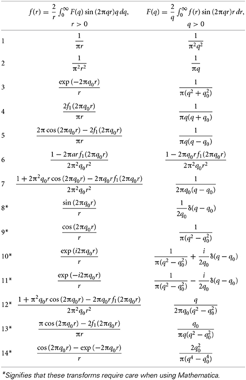
Table 1. Spherically-symmetric Fourier transform pairs in 3D.

The first is f_H (r) = sin (2πq₀ r)/r. Then

$\begin{array}{cc}\begin{array}{l}{F}_H(q)=\frac{2}{q}{\displaystyle {\int }_0^{\infty }\sin }(2\pi q_{0}r)\sin (2\pi qr)\text{d}r\\ =\frac{1}{q}{\displaystyle {\int }_{-\infty }^{\infty }\sin }(2\pi q_{0}r)\sin (2\pi qr)\text{d}r,\end{array}& \left(14\right)\end{array}$

as the integrand is an even function. Introducing the complex forms for the trigonometric functions, we obtain

$\begin{array}{cc}\begin{array}{l}\frac{\sin (2\pi q_{0}r)}{r}\iff \frac{1}{4q}{\displaystyle {\int }_{-\infty }^{\infty }\{\exp \left[i2\pi (q-q_0)r\right]}\\ +\exp \left[-i2\pi (q-q_0)r\right]-\exp \left[i2\pi (q+q_0)r\right]\\ -\exp \left[-i2\pi (q+q_0)r\right]\}\text{d}r\\ =\frac{1}{2q}[\delta (q-q_0)-\delta (q+q_0)]=\delta (q^2-q_0^2),\end{array}& \left(15\right)\end{array}$

using the properties of the Dirac delta function δ ( · )[2]. As q is positive definite, δ (q + 1/λ) vanishes upon integration over positive q, so effectively

$\begin{array}{cc}\frac{\sin (2\pi q_{0}r)}{r}\iff \frac{1}{2q_0}\delta (q-q_0).& \left(16\right)\end{array}$

The inverse transform follows directly from substituting the delta function into Equation 13. This transform, which corresponds to our homogeneous solution in Equation 3, does not appear in many of the standard tables, nor does Mathematica incorporate it. But it is frequently used to describe propagating waves in diffraction crystallography [25], grating theory [26, 27], diffraction and imaging theory [28, 29], holographic reconstruction [30], and tomography [31, 32]. It has been very successful in calculation of focused fields, analysis of imaging systems, and in tomographic reconstruction. Then δ (q − 1/λ) describes the surface of a sphere in reciprocal space or k-space, that represents the property that the magnitude of the wave vector is fixed at a real value k = k₀, where k₀ = 2π /λ = 2πq₀, as illustrated in Figure 1A.

FIGURE 1

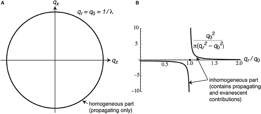
Figure 1. (A) The homogeneous part of the Green function transform (Equation 16) resides on a spherical shell of radius q₀ in q space, and is imaginary in value. The radius q_r is positive. (B) The inhomogeneous part of the Green function transform (Equation 20) is positive outside of the sphere radius q₀, zero on the sphere, and negative inside the sphere.

The McCutchen sphere and the Ewald sphere

In optics, McCutchen introduced the generalized pupil, which is a cap of a sphere of radius equal to the focal length of a lens [28]. Then in the Debye approximation the amplitude in the focal region of the lens, when illuminated by a plane wave, is given by the 3D Fourier transform of the generalized pupil. The fact that the coherent transfer function (CTF) (in spatial frequency space) is a scaled version of the pupil is well known in 2D Fourier optics [33]; so analogously in 3D, the 3D CTF is a scaled version of the 3D (generalized) pupil. A related concept is the Ewald sphere of diffraction crystallography, but more accurately the Ewald sphere represents the scattering vector rather than the wave vector, and so as a result the sphere is shifted so that it passes through the origin of reciprocal space rather than having its center at the origin. The McCutchen construction has the advantage over the Fresnel approximation that it is by nature non-paraxial. It has been shown that the concept of the generalized pupil can be extended to the finite Fresnel number case [5, 7, 8], to electromagnetic focusing [6, 34], and to pulsed waves [35, 36].

The term in Equation 15 is a solution of the homogeneous Helmholtz equation (Equation 3) and for this reason we call it the homogeneous component of the Green function. It is made up of only propagating plane waves (which we define to include combinations that give standing waves), and contains no evanescent part. It is divergence-free. For the complete spherical shell δ (q − 1/λ), the propagating waves combine to give a pure standing wave structure. This is the simple physical example of focusing of a complete spherical in-going wave, which in free space subsequently expands to form an out-going wave [37, 38]. Physically, we can recognize that a point in q space represents a propagating plane wave, which propagates inwards from infinity, before passing the origin and then propagating outwards toward infinity. This is not the same as an out-going wave. Two points in q space, diametrically opposite each other with respect to the origin, add together to produce a standing wave fringe pattern, and then integrating over such fringe patterns with different orientations gives a focused spot. At the focal point all the plane waves add in phase to produce a maximum in amplitude. This case corresponds to a source in conjunction with a sink. A sink we usually assume cannot exist alone in the real world (unless produced as a result of a drain, or an outlet [9]). A few recent papers seem to have missed the point that isolated sinks do not physically occur in free space [39]. Note that although the transform is represented as an integral of a real function along the positive real axis, the result, if an analytic function, can be continued analytically to complex frequencies, or in the case of the inverse transform to complex positions. In complex source-point theory, due account needs to be taken of branch cuts, appropriate choice of which can produce beam-like or source-like solutions [40, 41]. A source-sink pair is the basis of a version of a complex source point model of Gaussian beams that avoids non-physical singularities [42, 43].

The inhomogeneous solution, continued

Our second important example of a function is f_I (r) = cos (2πq₀ r)/r. Then we have

$\begin{array}{cc}{F}_I(q)=\frac{2}{q}{\displaystyle {\int }_0^{\infty }\cos }(2\pi q_{0}r)\sin (2\pi qr)\text{d}r.& \left(17\right)\end{array}$

This integral can be evaluated in several different ways. One such way is to use the properties of the Heaviside step function and the signum function, sgn( · )[17]. Then, introducing the complex forms for the trigonometric functions,

$\begin{array}{cc}\begin{array}{l}{F}_I(q)=\frac{1}{i4\pi q}{\displaystyle {\int }_{-\infty }^{\infty }s}gn(r)\{\exp \left[i2\pi (q-q_0)r\right]\\ -\exp \left[-i2\pi (q-q_0)r\right]+\exp \left[i2\pi (q+q_0)r\right]\\ -\exp \left[-i2\pi (q+q_0)r\right]\}\text{d}r,\end{array}& \left(18\right)\end{array}$

and, using the Fourier transform of the signum function and the shift theorem, we obtain

$\begin{array}{cc}{F}_I(q)=\frac{1}{2\pi q}\left(\frac{1}{q+q_0}+\frac{1}{q-q_0}\right)=\frac{1}{\pi \left(q^2-q_0^2\right)}.& \left(19\right)\end{array}$

The inverse transform can be obtained rigorously as shown by Lighthill [16], giving the transform pair,

$\begin{array}{cc}\frac{\cos (2\pi q_{0}r)}{r}\iff \frac{1}{\pi \left(q^2-q_0^2\right)}.& \left(20\right)\end{array}$

Again this transform is not in some standard tables. (But it is in [18], [20], and [19]). In fact it differs from the standard (complex) result for the inverse transform, obtained using contour integration by assuming q²₀ has a small positive imaginary part. As the solution in Equation 19 is obtained by Fourier transformation of the inhomogeneous Helmholtz equation we call it the inhomogeneous part of the Green function (Figure 1B). Note that this terminology is different from a usual connotation of inhomogeneous waves, as being synonymous with evanescent waves. In the SSFT the kernel is real, so we would expect the transform of a real function to also be real. Further, the functions on both sides of Equation 20 are spherically symmetric in 3D space, and hence their projections on to the r, q axes are even functions. By the projection-slice theorem of Fourier transforms, neither function should give rise to a complex transform. Thus, the homogeneous and inhomogeneous parts of the Green function transform are as illustrated in Figures 1A,B, respectively.

Out-Going and In-Going Waves

The out-going wave and causality

We can combine the results of Equations 15 and 19 to give the transform pair

$\begin{array}{cc}\frac{\exp (i2\pi q_{0}r)}{r}\iff \frac{1}{\pi \left(q^2-q_0^2\right)}+i\delta \left(q^2-q_0^2\right).& \left(21\right)\end{array}$

With q₀ = 1/λ, this represents an outgoing spherical wave, or source, equivalent to the Green function or impulse response. Dirac showed [2], that an out-going wave (or particle) must have a Fourier transform of this form in order to satisfy causality [17]. Causality requires that the real and imaginary parts satisfy a Hilbert transform relationship [10, 12, 44, 45], as in the Kramers-Kronig relations for dispersion. In the present paper, causality also applies in space, rather than in time, because of the single-sided form of polar coordinates. Note that Jackson uses the causal form in his treatment of dispersion, and even comments on its usefulness, but does not introduce it for the Green function in space [12]. In mathematics the form in Equation 21 is known as the Sokhotsky-Plemelj formula.

On-shell and off-shell, and Bragg diffraction

The two terms of Equation 21 are equivalent to the off-shell and on-shell conditions, respectively, in quantum field theory. Virtual particles are allowed to be off shell. The connection between virtual photons and evanescent waves has been discussed [46, 47]. Lawson describes how there are two different types of virtual photon, corresponding to real off-shell values of k, and complex k, respectively. In this Section we are concerned with the first type [46]. According to Lawson, values k > k₀, i.e., when the momentum is greater than the energy associated with it, correspond to virtual photons with negative mass, and are “spacelike.” When k < k₀, i.e., when the momentum is less than the energy associated with it, the virtual photons have positive mass, and are ‘timelike.’ The second type of virtual photon, with complex k, corresponds with classical evanescent waves, as in Section Forward and Backward Propagating Waves.

The on-shell part of Equation 21 corresponds to satisfaction of the Bragg diffraction condition. If this term alone existed, there would be no off-Bragg diffraction. In grating diffraction, off-Bragg diffraction is modeled using k-vector closure, which assumes the diffracted wave has slightly different value of q, or by the so-called β-value method, which introduces a dephasing measure [26]. In dynamical theory of diffraction, a deformation of the k-space sphere (dispersion surface) occurs, analogous to the splitting of energy levels in quantum theory [25]. The inhomogeneous part can be interpreted as describing the dispersion of free space, a resonance phenomenon associated with an impulsive source.

As q is positive definite, δ (q + q₀) vanishes upon integration over positive q. So effectively we can write

$\begin{array}{cc}\begin{array}{l}\frac{\exp (i2\pi q_{0}r)}{r}\iff \frac{1}{2\pi q_0(q-q_0)}-\frac{1}{2\pi q_0(q+q_0)}\\ +\frac{i}{2q_0}\delta \left(q-q_0\right).\end{array}& \left(22\right)\end{array}$

Regularization

In the classic physics and electromagnetic books [11, 12], the homogeneous solution is not written explicitly, but can be recovered by treating q as complex and choosing an appropriate integration contour. Then Equation 21 (or Equation 22) can be recognized as showing explicitly the real and imaginary parts of F(q). The real part is the Cauchy principal value of the function at q = q₀, so we should write F_I (q) = P[1/π(q² − q²₀)], where P means principal part. An equivalent approach is to introduce explicitly a non-physical small imaginary part [48], giving

$\begin{array}{cc}\begin{array}{l}{F}_I(q)=\underset{\epsilon \to 0^{+}}{\text{Lim}}\left[\frac{1}{\pi (q^2-q_0^2-i\epsilon )}\right]\\ =\underset{\epsilon \to 0^{+}}{\text{Lim}}\left\{\frac{(q^2-q_0^2)}{\pi [{(q^2-q_0^2)}^2+{\epsilon }^2]}+\frac{i\epsilon }{\pi [{(q^2-q_0^2)}^2+{\epsilon }^2]}\right\}\\ =\frac{1}{\pi (q^2-q_0^2)}+i\underset{\epsilon \to 0^{+}}{\text{Lim}}\left\{\frac{\epsilon }{\pi [{(q^2-q_0^2)}^2+{\epsilon }^2]}\right\}\\ =\frac{1}{\pi (q^2-q_0^2)}+i\delta (q^2-q_0^2),\end{array}& \left(23\right)\end{array}$

as before. This is a form of regularization, widely used in inverse problems, similar to that used in renormalization theory. The imaginary part of Equation 23, the second term of Cauchy-Lorentz form, gives a delta function in the limit, and represents solely propagating waves. Evanescent waves are contained in the real part only (first term), which exhibits a singularity. Sometimes the expression for F_I (q) as given in Equation 19 is understood to include implicitly the imaginary part, i.e., q (and therefore λ) is assumed complex. But as Equation 19 exhibits a branch cut along the real axis, we prefer to take both q and q₀ as real and positive. Then according to Hankel's theorem [49] the value of the transform for real q is equal to the mean of the values of the transform for ε → 0⁺ and ε → 0⁻, just as we normally assume in deriving Fourier series. The integral is then equivalent to the Cauchy principal value.

In-going waves

In a similar manner, for an in-going rather than an out-going wave,

$\begin{array}{cc}\frac{\exp (-i2\pi q_{0}r)}{r}\iff \frac{1}{\pi \left(q^2-q_0^2\right)}-i\delta \left(q^2-q_0^2\right).& \left(24\right)\end{array}$

This corresponds to a sink, which as we have said, we usually assume cannot exist alone in the real world. This assumption is equivalent to the Sommerfeld radiation condition [13, 14]. But a sink can exist physically in free space in conjunction with a source, as together they can combine to give the homogeneous part alone, which exhibits no singularity in the spatial domain. We recognize that

$\begin{array}{cc}\begin{array}{l}\frac{1}{\pi \left(q^2-q_0^2\right)}\iff \frac{\cos (2\pi q_{0}r)}{r}\\ =\frac{1}{2}\left[\frac{\exp (i2\pi q_{0}r)}{r}+\frac{\exp (-i2\pi q_{0}r)}{r}\right],\end{array}& \left(25\right)\end{array}$

also represents a combination of an out-going and an in-going wave, each of which includes both propagating and evanescent components.

Homogeneous and Inhomogeneous Waves, vs. Traveling and Evanescent Waves

The homogeneous component in Equation 5 contains only propagating components. It is a special case of the Whittaker expansion over propagating plane waves traveling in all directions, corresponding to a complete sphere in Fourier space [50]. This should be contrasted with the Weyl expansion, which is an expansion over a half-space, giving a hemisphere of propagating waves, and evanescent waves [51]. The Weyl expansion for the scalar Green function was presented by Carter [52]: the evanescent field contains components for (q²_x + q²_y) > 1/λ only, whereas in Equation 20 q can be greater than or less than 1/λ. An analytic expression for the propagating and evanescent components was given by Bertilone [53, 54]. The Green function in Equation 21 is made up of a real inhomogeneous part and an imaginary homogeneous part. Here “homogeneous” and “inhomogenous” refer to corresponding forms of the Helmholtz equation. We thus distinguish between “inhomogeneous” and “evanescent” components. Both homogeneous and inhomogeneous parts contribute to the far field, but only the inhomogeneous component contributes to the near-field singularity [55]. Each propagating component in the Weyl expansion contains inhomogeneous, as well as homogeneous, components when considered in 3D, because for a point source a propagating plane wave component exhibits a discontinuity at the source, being out-going on both sides.

Forward and Backward Propagating Waves

We now explore the result of introducing a specific orientation. The inhomogeneous part of the transform of the Green function 1/[π(q² − q²₀)] contains components for q < 1/λ in addition to those for q > 1/λ, and also contains propagating as well as evanescent components. Putting

$\begin{array}{cc}(q^2-q_0^2)=\left[q_z-{(q_0^2-q_x^2-q_y^2)}^{1/2}\right]\left[q_z+{(q_0^2-q_x^2-q_y^2)}^{1/2}\right],& \left(26\right)\end{array}$

and using partial fractions, the transform of the Green function can be written in the form [7, 8, 56]

$\begin{array}{cc}\begin{array}{l}F(q_x,q_y,q_z)=\frac{i}{2\left|q_z\right|}[\delta \left(q_z-\sqrt{q_0^2-q_x^2-q_y^2}\right)\\ +\frac{1}{2\pi q_z\left(q_z-\sqrt{q_0^2-q_x^2-q_y^2}\right)}\\ +\delta \left(q_z+\sqrt{q_0^2-q_x^2-q_y^2}\right)\\ +\frac{1}{2\pi q_z\left(q_z+\sqrt{q_0^2-q_x^2-q_y^2}\right)}].\end{array}& \left(27\right)\end{array}$

Here the homogeneous part (the first and third terms) is written as the sum of two unweighted hemispherical shells in reciprocal space, representing forward and backward propagating waves, respectively. The total transform has only out-going propagating components, so the inhomogeneous part (the second and fourth terms) must also include propagating components. We thus distinguish between forward and backward propagating waves on the one hand, and out-going and in-going waves on the other. A forward propagating wave is in-going for z < 0, and out-going for z > 0. Some papers have confused causality with forward propagation [57]: of course a backward propagating wave is physically realizable, as all it needs is a reversal of the z coordinate.

Each of the inhomogeneous terms in Equation 27 contain components with q_z > 0 and q_z <0. For (q²_x + q²_y) < 1/λ² these terms each represent both out-going and in-going propagating waves, which for z > 0 together with the homogeneous terms result in a purely out-going, forward-propagating field, represented by a hemispherical shell in reciprocal space,

$\begin{array}{cc}{F}_{FP}(q_x,q_y,q_z)=\frac{i}{\left|q_z\right|}\delta \left(q_z-\sqrt{q_0^2-q_x^2-q_y^2}\right).& \left(28\right)\end{array}$

as shown in Figure 2A. This spherical surface, which includes contributions from both the homogeneous and inhomogeneous parts, is therefore not the same as McCutchen's spherical surface of homogeneous waves, and in fact has a strength twice that of the homogeneous component. This is an important property of our present treatment: using the hemispherical shell from the homogeneous part alone would give half the correct result for the diffracted field.

FIGURE 2

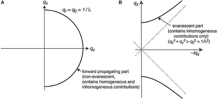
Figure 2. (A) The Green function transform for forward propagating (non-evanescent) waves for observation points z > 0 lies on a hemispherical shell. It consists of contributions from both the homogeneous and inhomogeneous parts of the Green function transform in 3D (Equation 28). (B) The evanescent part of the Green function transform resides on a hyperboloid of one sheet in q_x, q_y, − iq_z space (Equation 30).

For a source at the origin z = 0, the Weyl expansion can be applied separately for the regions z < 0, and for z > 0. The propagating field is then out-going, and there is also an evanescent field in both regions. But it is incorrect to think of these components as adding together to give the total field, as the expansion for z > 0 gives a field for z < 0, and vice-versa. So adding together Weyl expansions for the two half-spaces does not give the total field.

For q²_x + q²_y > 1/λ², the inhomogeneous terms in Equation 27 transform to

$\begin{array}{cc}\begin{array}{l}{f}_E(x,y,z)=i{\displaystyle \iint \frac{1}{q_z}}\exp [i2\pi \left(q_{x}x+q_{y}y\right)\\ -2\pi {\left(q_x^2+q_y^2-q_0^2\right)}^{1/2}\left|z\right|]\text{d}{q}_x\text{d}{q}_y\end{array}& \left(29\right)\end{array}$

and are hence equivalent to the evanescent waves of the Weyl expansion. As this is true for any choice of z direction, we conclude that the evanescent field is completely contained in the part of the inhomogenous field corresponding to q > 1/λ. Note, however, this part for q > 1/λ also includes components with (q²_x + q²_y) < 1/λ² which contributes to the propagating field. The homogeneous terms in Equation 27 are not, by themselves, equivalent to the (out-going) propagating components of the Weyl expansion. A fuller discussion of the significance of introducing a fixed reference direction, and calculation of fields for positive z only, has been presented elsewhere [7, 8].

As for z > 0 an exponential decay is also produced by a transform of the form δ (−iq_z + (q²_x + q²_y − 1/λ²)^1/2), we can write for the evanescent field

$\begin{array}{cc}\begin{array}{l}{F}_E(q_x,q_y,q_z)=\frac{i}{q_z}\delta \left(q_z-\sqrt{q_0^2-q_x^2-q_y^2}\right),{\left(q_x^2+q_y^2\right)}^{1/2}\\ <q_0,q_z>0\&z>0,\\ =\frac{1}{-i{q}_z}\delta \left(-i{q}_z+\sqrt{q_x^2+q_y^2-q_0^2}\right),{\left(q_x^2+q_y^2\right)}^{1/2}\\ >q_0,-i{q}_z>0\&z>0.\end{array}& \left(30\right)\end{array}$

Although the properties of delta function with complex argument may not be well established, here the argument of the delta function is −iq_z which is real, and we interpret the result as integration over a rectangular hyperboloid of one sheet in a spatial frequency space (q_x, q_y, −iq_z), as illustrated in Figure 2B. Thus, the full Rayleigh-Sommerfeld diffraction formula can be applied exactly, including evanescent waves, using 3D Fourier transforms, and evaluated numerically.

Combining the Whittaker and Weyl Expansions

The Weyl expansion represents an out-going spherical wave in terms of an angular spectrum of plane waves [51]. As the out-going spherical wave exhibits a singularity at its origin, the expansion must include evanescent components. Evanescent waves are not valid over a full, infinite space, so the expansion is limited to a half-space. The Whittaker expansion represents a singularity-free spherical standing wave in terms of angular spectra of in-going and out-going plane waves over a complete sphere [50]. Out-going waves can include forward-propagating and backward-propagating components, and similarly for in-going waves. No evanescent components are necessary as there is no singularity. For some field distribtions, both the Whittaker and Weyl expansions are valid [58]. For example, a field consisting of forward-propagating, out-going waves in a half-space, with no evanescent waves. It seems that there should be some more general expansion, of which the Whittaker and Weyl expansions are special cases. Devaney and co-workers have attempted to reconcile the Weyl and Whittaker expansions, with some, but limited, success [58, 59]. We reconsider this problem in the light of our present treatment. We consider a few different forms of expansion, which shed light on the relationship between the two expansions, and show how the two expansions can be combined.

A Region of Space within a Closed Surface Free of Net Sources

Neglecting an evanescent field that may be present near to the outside surface, inside the region there are only propagating waves, equivalent to a sum over coincident source/sink combinations. This corresponds to a Whittaker expansion, a sum over out-going and in-going propagating components, equivalent to a divergence-free combination of sources and sinks (Figure 1A).

A Source-Free Half-Space with Forward Propagating Waves and Evanescent Waves

This corresponds to a Weyl expansion (Figures 2A,B).

A Finite Region of Space with Net Sources

We can combine the Weyl and Whittaker expansions by summing over a distribution of sources and sinks with non-zero divergence, giving a total homogeneous and inhomogeneous field. The homogeneous and inhomogeneous parts of the spatial frequency content are given by the filtered transform of the Green function, given by homogeneous and inhomogeneous components. As the homogeneous part is non-zero on the k-space sphere only, different source/sink distributions can give rise to the same homogeneous field, but the source/sink distribution is uniquely determined by the inhomogeneous part. Relating the inhomogeneous part to the evanescent field requires selection of a reference direction z.

For a Region z > 0 that is Source Free, Any Field can be Generated by a Sum of Propagating and Evanescent Components

In addition to the components in the Weyl expansion, the propagating components in general include in-going fields equivalent to sources at infinity, which give no evanescent field for finite values of z. For a known field in the plane z = 0, the spectral distribution is a function of q_x, q_y only, which filters the transform corresponding to the Rayleigh-Sommerfeld kernel [7, 8]. For any distribution of sources and sinks with z < 0, the field for z > 0 can then be represented by an equivalent field in the plane z = 0. Note that we do not claim that the field in the region z < 0 can be determined in general by this approach. The Rayleigh hypothesis states that the field inside a re-entrant surface can be determined by analytic continuation. Recent numerical evidence and arguments based on transformation optics seem to support the hypothesis except in some pathological cases [60, 61].

A List of Spherically-Symmetric Fourier Transforms

A list of SSFTs is given in Table 1, based on the transforms given in Equations 16 and 20, rather than Equation 8, as is taken by Mathematica. We have introduced the auxiliary functions of the sine and cosine integrals, f₁ (x) = Ci(x) sin x − si(x) cos (x), where si(x) = Si(x) − π/2. f₁ (x) decreases monotonically from π/2, as shown in Figure 3. The first four entries in the table are well known. Nos. 8–11 we have already discussed. Then Nos. 5–7 follow from 1–4 and 9. Nos. 12–14 can be derived consistently from Nos. 1–11. Some of these transforms can be generated directly using Mathematica's FourierSinTransform function. Important exceptions are Nos. 8–11, and transforms derived from them, which also do not appear in many published tables of transforms. Cases in which care is needed in applying Mathematica are indicated by an asterisk.

FIGURE 3

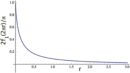
Figure 3. The normalized value of f₁, showing that it decays monotonically.

Summary

In summary, we have examined the Fourier transform of Green function in its own right in contrast to the standard approach in theoretical physics and electromagnetism, which uses the transform of the Green function only as a step on the way to finding the Green function in real space. The transform is written in a form where the homogeneous part is shown explicitly as a delta function representing a spherical shell, and the inhomogeneous part contains spatial frequencies with q < q₀ as well as q > q₀. Both homogeneous and inhomogeneous parts include propagating components, and the singularity of the Green function is contained completely in the inhomogeneous part for q > q₀.

If a particular direction of propagation is assumed, for z > 0 the transform consists of a hemispherical shell representing forward-propagating waves and part of a rectangular hyperboloid of one sheet for imaginary q_z representing forward-directed evanescent waves. An analogous behavior holds for z < 0, but the two hemispheres cannot be considered together as equivalent to the homogeneous sphere because the hemisphere for z > 0 also gives a field for z < 0, and vice-versa. The interpretation helps us appreciate the connection between the forward scattering model, and the use of the Ewald sphere approach in the inverse problem of crystallographic and tomographic reconstruction.

Finally, our paper has been confined to the treatment of scalar waves, but extension to the full electromagnetic case is straightforward, based on the use of the scalar Whittaker potentials, equivalent to the dyadic Green function [48, 62–66].

Conflict of Interest Statement

The authors declare that the research was conducted in the absence of any commercial or financial relationships that could be construed as a potential conflict of interest.

Acknowledgments

Colin J. R. Sheppard thanks the University of Melbourne for a Lyle Fellowship. Shan S. Kou and Jiao Lin are recipients of the Discovery Early Career Researcher Award funded by the Australian Research Council under projects DE120102352 and DE130100954, respectively. Shan S. Kou acknowledges the financial support from the Melbourne Collaboration Grant and the Interdisciplinary Seed Fund through the Melbourne Materials Institute (MMI). Jiao Lin acknowledges the financial support from the Defence Science Institute, Australia.

References

1. Schmalz JA, Schmalz G, Gureyev TE, Pavlov KM. On the derivation of the Green's function for the Helmholtz equation using generalized functions. Am J Phys. (2010) 78:181–6. doi: 10.1119/1.3253655

CrossRef Full Text | Google Scholar

2. Dirac PAM. The Principles of Quantum Mechanics. Oxford: Oxford University Press (1981).

Google Scholar

3. Heitler W. The Quantum Theory of Radiation. Oxford: Clarendon Press (1936).

Google Scholar

4. Mandel L, Wolf E. Optical Coherence and Quantum Optics. Cambridge: Cambridge University Press (1995). doi: 10.1017/CBO9781139644105

CrossRef Full Text | Google Scholar

5. Lin J, Yuan XC, Kou SS, Sheppard CJR, Rodríguez-Herrera OG, Dainty JC. Direct calculation of a three-dimensional diffraction field. Opt Lett. (2011) 36:1341–3. doi: 10.1364/OL.36.001341

Pubmed Abstract | Pubmed Full Text | CrossRef Full Text | Google Scholar

6. Lin J, Rodriguez-Herrera OG, Kenny F, Lara D, Dainty JC. Fast vectorial calculation of the volumetric focused field distribution by using a three- dimensional Fourier transform. Opt Exp. (2012) 20:1060–9. doi: 10.1364/OE.20.001060

Pubmed Abstract | Pubmed Full Text | CrossRef Full Text | Google Scholar

7. Sheppard CJR, Lin J, Kou SS. Rayleigh–Sommerfeld diffraction formula in k space. J Opt Soc Am A (2013) 30:1180–3. doi: 10.1364/JOSAA.30.001180

Pubmed Abstract | Pubmed Full Text | CrossRef Full Text | Google Scholar

8. Kou SS, Sheppard CJR, Lin J. Evaluation of the Rayleigh-Sommerfeld diffraction formula with 3D convolution: the 3D angular spectrum (3D-AS) method. Opt Lett. (2013) 38:5296–9. doi: 10.1364/OL.38.005296

Pubmed Abstract | Pubmed Full Text | CrossRef Full Text

9. Tyc T, Zhang X. Perfect lenses in focus. Nature (2011) 480:42–3. doi: 10.1038/480042a

Pubmed Abstract | Pubmed Full Text | CrossRef Full Text | Google Scholar

10. Titchmarsh EC. Introduction to the Theory of Fourier Integrals, 2nd Edn. Oxford: Clarendon Press (1948).

Google Scholar

11. Morse PM, Feshbach H. Methods of Theoretical Physics. New York, NY: McGraw Hill (1978).

Google Scholar

12. Jackson JD. Classical Electrodynamics. New York, NY: John Wiley and Sons (1962).

Google Scholar

13. Sommerfeld A. Partial Differential Equations in Physics. Pure and Applied Mathematics. New York, NY: Academic Press (1949).

Google Scholar

14. Schot S. Eighty years of Sommerfeld's radiation condition. Hist Math. (1992) 19:385–401. doi: 10.1016/0315-0860(92)90004-U

CrossRef Full Text | Google Scholar

15. Temple G. The theory of generalized functions. Proc R Soc Lond A (1955) 228:175–90. doi: 10.1098/rspa.1955.0042

CrossRef Full Text | Google Scholar

16. Lighthill MJ. Introduction to Fourier Analysis and Generalised Functions. Cambridge: Cambridge University Press (1958).

Google Scholar

17. Bracewell RN. The Fourier Transform and its Applications, McGraw-Hill Electrical and Electronic Engineering Series. New York, NY: McGraw Hill (1978).

18. Erdélyi A. (ed.). Tables of Integral Transforms. Vol. 1. New York, NY: McGraw Hill (1954).

Google Scholar

19. Oberhettinger F. Tables of Fourier Transforms, and Fourier Transforms of Distributions. Berlin: Springer (1990). doi: 10.1007/978-3-642-74349-8

CrossRef Full Text | Google Scholar

20. Poularikas AD. The Transforms and Applications Handbook, 2nd Edn. Boka Raton, FL: CRC Press (2000). doi: 10.1201/9781420036756

CrossRef Full Text | Google Scholar

21. Polyanin AD. Available online at: http://eqworld.ipmnet.ru/en/auxiliary/aux-inttrans.htm (2005).

22. eFunda. Available online at: http://www.efunda.com/math/Fourier_transform/table.cfm?TransName=Fs (2012).

23. Abramowitz M, Stegun I. Handbook of Mathematical Functions, 3rd Edn. New York, NY: Dover (1972).

Google Scholar

24. Gradshteyn IS, Ryzhik IM. Tables of Integrals, Series, and Products. New York, NY: Academic Press (1994).

Google Scholar

25. James RW. The Optical Principles of the Diffraction of X-rays. London: Bell (1948).

26. Kogelnik H. Coupled wave theory for thick hologram grating. Bell Syst Tech J. (1969) 48:2909–47. doi: 10.1002/j.1538-7305.1969.tb01198.x

Pubmed Abstract | Pubmed Full Text | CrossRef Full Text | Google Scholar

27. Sheppard CJR. The application of the dynamical theory of x-ray diffraction to thick hologram gratings. Int J Elect. (1976) 41, 365–73. doi: 10.1080/00207217608920647

CrossRef Full Text | Google Scholar

28. McCutchen CW. Generalized aperture and the three-dimensional diffraction image. J Opt Soc Am. (1964) 54:240–4. doi: 10.1364/JOSA.54.000240

CrossRef Full Text | Google Scholar

29. Sheppard CJR. The spatial frequency cut-off in three-dimensional imaging. Optik (1986) 72:131–3.

Google Scholar

30. Wolf E. Three-dimensional structure determination of semi-transparent objects from holographic data. (1969) Optics Comm. 1:153–6. doi: 10.1016/0030-4018(69)90052-2

CrossRef Full Text | Google Scholar

31. Dändliker R, Weiss K. Reconstruction of the three-dimensional refractive index from scattered waves. Optics Comm. (1970) 1:323–8. doi: 10.1016/0030-4018(70)90032-5

Pubmed Abstract | Pubmed Full Text | CrossRef Full Text | Google Scholar

32. Devaney AJ. Inversion formula for inverse scattering within the Born approximation. Opt Lett. 7:111–3. (1982). doi: 10.1364/OL.7.000111

Pubmed Abstract | Pubmed Full Text | CrossRef Full Text | Google Scholar

33. Goodman JW. Introduction to Fourier Optics. New York, NY: McGraw-Hill (1968).

Google Scholar

34. Sheppard CJR, Larkin KG. Vectorial pupil functions and vectorial transfer functions. Optik (1997) 107:79–87.

Pubmed Abstract | Pubmed Full Text | Google Scholar

35. Sheppard CJR, Sharma MD. Spatial frequency content of ultrashort pulsed beams. J Optics A Pure Appl Opt. (2002) 4:549–52. doi: 10.1088/1464-4258/4/5/310

CrossRef Full Text | Google Scholar

36. Sheppard CJR. Generalized Bessel pulse beams. J Opt Soc Am A (2002) 19:2218–22. doi: 10.1364/JOSAA.19.002218

Pubmed Abstract | Pubmed Full Text | CrossRef Full Text | Google Scholar

37. van der Pol B. On potential and wave functions in n dimensions. Physica (1936) 3:385–92. doi: 10.1016/S0031-8914(36)80003-2

CrossRef Full Text | Google Scholar

38. Sheppard CJR, Matthews HJ. Imaging in high aperture optical systems. J Opt Soc Am A (1987) 4:1354–60. doi: 10.1364/JOSAA.4.001354

CrossRef Full Text | Google Scholar

39. Leonhardt U. Perfect imaging without negative refraction. New J Phys. (2009) 11:093040. doi: 10.1088/1367-2630/11/9/093040

CrossRef Full Text | Google Scholar

40. Kaiser G. Complex-distance potential theory and hyperbolic equations. In: JRAW Sprössig, editors. Clifford Analysis. Boston, MA: Birkhäuser. (2000), 135–69.

41. Sheppard CJR. High-aperture beams: reply to comment. J Opt Soc Am A (2007) 24:1211–3. doi: 10.1364/JOSAA.24.001211

CrossRef Full Text | Google Scholar

42. Berry MV. Evanescent and real waves in quantum billiards and Gaussian beams. J Phys A (1994) 27:L391–8. doi: 10.1088/0305-4470/27/11/008

CrossRef Full Text | Google Scholar

43. Sheppard CJR, Saghafi S. Beam modes beyond the paraxial approximation: a scalar treatment. Phys Rev A (1998) 57:2971–9. doi: 10.1103/PhysRevA.57.2971

Pubmed Abstract | Pubmed Full Text | CrossRef Full Text | Google Scholar

44. Wiener N. Generalized harmonic analysis. Acta Math. (1930) 55:117–258. doi: 10.1007/BF02546511

CrossRef Full Text | Google Scholar

45. Gabor D. Theory of communication. J. IEEE (1946) 93:429–57.

Pubmed Abstract | Pubmed Full Text | Google Scholar

46. Lawson JD. Some attributes of real and virtual photons. Contemp. Phys. (1970) 11:575–80. doi: 10.1080/00107517008202195

CrossRef Full Text | Google Scholar

47. Stahlhofen AA, Nimtz G. Evanescent waves are virtual photons. Europhys. Lett. (2006) 76:189. doi: 10.1209/epl/i2006-10271-9

Pubmed Abstract | Pubmed Full Text | CrossRef Full Text | Google Scholar

48. Arnoldus H. Representation of the near-field, middle-field, and far-field electromagnetic Green's functions in reciprocal space. J Opt Soc Am B (2001) 18:547–55. doi: 10.1364/JOSAB.18.000547

CrossRef Full Text | Google Scholar

49. Watson GN. A Treatise on the Theory of Bessel Functions. Cambridge: Cambridge University Press (1980).

Google Scholar

50. Whittaker ET. On the partial differential equations of mathematical physics. Mathematische Annalen (1903) 57:333–55.

Google Scholar

51. Weyl H. Ausbreitung elektromagnetische Wellen über einem ebenen Leiter. Annalen Physik (1919) 365:481–500. doi: 10.1002/andp.19193652104

CrossRef Full Text | Google Scholar

52. Carter WH. Band-limited angular spectrum approximating to a spherical wave field. J Opt Soc Am. (1975) 65:1054–8. doi: 10.1364/JOSA.65.001054

CrossRef Full Text | Google Scholar

53. Bertilone DC. The contributions of homogeneous and evanescent plane waves to the scalar optical field : exact diffraction formulae. J Mod Opt. (1991) 38:865–75. doi: 10.1080/09500349114550851

Pubmed Abstract | Pubmed Full Text | CrossRef Full Text | Google Scholar

54. Bertilone DC. Wave theory for a converging spherical incident wave in an infinite-aperture system. J Mod Opt. (1991) 38:1531–6. doi: 10.1080/09500349114551701

CrossRef Full Text | Google Scholar

55. Sheppard CJR, Aguilar JF. Evanescent fields do contribute to the far field. J Mod Opt. (1999) 46:729.–comment: J Mod Optics (2001) 48:177–80. doi: 10.1080/09500340108235163

CrossRef Full Text | Google Scholar

56. Sheppard CJR, Fatemi H, Gu M. The Fourier optics of near-field microscopy. Scanning (1995) 17:28–40. doi: 10.1002/sca.4950170105

CrossRef Full Text | Google Scholar

57. Heyman E. Focus wave modes: a dilemma with causality. IEEE Trans Antennas Prop. (1989) AP-37:1604–8. doi: 10.1109/8.45104

CrossRef Full Text | Google Scholar

58. Devaney AJ, Sherman G. C. Plane-wave representations for scalar wave fields. SIAM Rev. (1973) 15:765–86. doi: 10.1137/1015096

CrossRef Full Text | Google Scholar

59. Devaney AJ, Wolf E. Multipole expansions and plane wave representations of the electromagnetic field. J Math Phys. (1974) 15:234–44. doi: 10.1063/1.1666629

CrossRef Full Text | Google Scholar

60. Tishchenko AV. Numerical demonstration of the validity of the Rayleigh hypothesis. Opt Express (2009) 17:17102–17. doi: 10.1364/OE.17.017102

Pubmed Abstract | Pubmed Full Text | CrossRef Full Text | Google Scholar

61. Tishchenko AV. Rayleigh was right: electromagnetic fields and corrugated interfaces. Opt Photon News (2010) 21:51–4. doi: 10.1364/OPN.21.7.000050

CrossRef Full Text | Google Scholar

62. Whittaker ET. On an expression of the electromagnetic field due to electrons by means of two scalar potential functions. Proc Lond Math Soc. (1904) 1:367–72. doi: 10.1112/plms/s2-1.1.367

CrossRef Full Text | Google Scholar

63. Nisbet A. Hertzian electromagnetic potentials and associated gauge transformations. Proc R Soc Lond Ser. A (1955) 231:250–63.

Google Scholar

64. Wilcox CH. Debye potentials. J. Math. Mech. (1957) 6:167–201.

65. Chew WC. Waves and Fields in Homogeneous Media. Piscataway, NJ: IEEE Press (1990).

Google Scholar

66. Sheppard CJR. Focal distributions and Hertz potentials. Optics Comm. (1999) 160:191–4. doi: 10.1016/S0030-4018(98)00647-6

CrossRef Full Text | Google Scholar