Discrete element modeling of brittle crack roughness in three dimensions

1. Introduction

The modern academic interest in crack morphology can be traced back to Mandelbrot et al. who introduced a mathematical framework for describing rough surfaces in terms of fractal geometry [1]. Specifically, crack surfaces have been shown to be self-affine in the sense that they satisfy certain scaling laws, where a characteristic exponent governs the asymptotic behavior [2]. This means that a scaling of lengths with a factor λ within the fracture plane implies that lengths perpendicular to this plane scale with a factor λ^ζ. Understanding fundamental aspects of crack roughness is also important in the engineering fields. Such is the case in the oil industry where flow properties within fractured rock masses is of great interest. Quantitative properties of crack surfaces are accessible through modern imaging techniques, and predictions of computer models [3, 4] can be compared with the results of practical experiments to verify or discard theoretical assumptions.

Much of the theoretical work done so far has been based on the random fuse model [5], i.e., a regular lattice of conducting elements which irreversibly burn out once their individual thresholds have been exceeded. Breakdown is driven by a voltage difference between two opposing boundaries and the analogy of Kirchhoff's equations with linear elasticity is the reason why this model is referred to as a scalar model of fracture. In two dimensions results reported for the roughness exponent with the fuse model are ζ = 0.74(2) [6, 7], and more recently ζ = 0.83(4) [8]. In three dimensions the random fuse model has yielded values in the range 0.4 ≲ ζ ≲ 0.6, i.e., Batrouni et al. obtained ζ = 0.62(5) [9], Räisänen et al. obtained ζ = 0.41(2) [10, 11], and Nukala et al. obtained ζ = 0.52(3) [12].

How do these results compare with experimental findings? Initially it was thought that the universal roughness exponent should be ζ ≃ 0.8 [2]. Later it was realized that there should instead exist two different regimes for the scaling behavior of cracks [13, 14]. It was proposed that a smaller exponent ζ ≃ 0.5 should be associated with short length scales and slow crack growth [15], while a larger exponent ζ ≃ 0.8 involving dynamic effects of fracture should be associated with longer length scales. The picture that has emerged more recently however is that, although there are indeed two scaling regimes, it is in fact the larger exponent ζ ≃ 0.8 which is relevant to short length scales. This is because of the screening of elastic interactions which takes place within the intermediate region between the crack tip and the surrounding medium, i.e., the fracture process zone. At larger length scales one observes ζ ≃ 0.45 [16, 17].

Roughly speaking, then, the three dimensional fuse model results are in agreement with what is obtained experimentally at large length scales. An important point to be considered with the fuse model, however, is the fact that it models electrical breakdown rather than fracture in a fully elastic medium. A different lattice model which incorporates elasticity is the Born-model [18]. Here the material is modeled as a network of elastic springs, each spring being free to rotate at its ends. In two dimensions ζ = 0.64(5) is obtained with this model [19]. As with the fuse model, this exponent is seen to drop somewhat when going from two to three dimensions. The result, ζ = 0.5 [20], is consistent with the range of exponents obtained with the random fuse model and agrees rather well with the scaling expected at length scales above those relevant to the fracture process zone.

A problem with the Born model is that it is not rotationally invariant [21]. A different model which does not suffer from this drawback is the elastic beam model [22, 23]. Here the beams are rigidly connected at the nodes so as to preserve the angle between any two neighboring beams. Rotations thus induce flexing and twisting deformations, while linear displacements induce transverse shear and axial forces. The exponent obtained with the beam model in two dimensions is ζ = 0.86(3) [24], and shows that the scalar and vectorial descriptions of fracture need not necessarily produce similar results, although the more recent two dimensional random fuse result of ζ = 0.83(4) quoted by Zapperi et al. [8] is consistent with this. Since the beam model provides a more realistic description of brittle elastic fracture than does either the fuse model or the Born model it is of great interest to see what the result is in three dimensions. An analogous study to this end has been made by Nukala et al. [25], obtaining both the global roughness exponent ζ = 0.48(3) and the local roughness exponent ζ_loc, which they find to be equal to the global roughness exponent for the beam lattice, ζ = ζ_loc. The local exponent in such cases is obtained by considering the scaling properties within “windows” of the crack surface for length scales l < < L, where L is the external size of the L × L × L lattice. Presently we only regard the global roughness exponent.

2. Model

Our model is a deformable lattice in the form of a regular cube with size L × L × L, where each node is connected to its nearest neighbors by linearly elastic beams. Forces acting on the nodes have been deduced from the effect a concentrated end-load has on a beam with no end-restraints [26, 27]. A coordinate system is placed on each node, and the enumeration of the connecting beams follows an anti-clockwise scheme within the XY-plane, i.e., beginning with the beam which lies along the positive X-axis and ending with that which extends upwards along the positive Z-axis, see Figure 1.

FIGURE 1

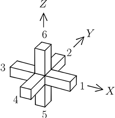
Figure 1. Enumeration scheme on the beams of a cube lattice connecting node i to its j = 1–6 nearest neighbors, showing the coordinate system with i as its origin.

At each stage of the breaking process, the updated displacements for each node is obtained from

$\begin{array}{cc}{\displaystyle \sum _j{D}_{ij}}\left[\begin{array}{l}{x}_i\hfill \\ y_i\hfill \\ z_i\hfill \\ u_i\hfill \\ v_i\hfill \\ w_i\hfill \end{array}\right]=\lambda \left[\begin{array}{l}{X}_i\hfill \\ Y_i\hfill \\ Z_i\hfill \\ U_i\hfill \\ V_i\hfill \\ W_i\hfill \end{array}\right],& (1)\end{array}$

which is solved iteratively via relaxation using the conjugate gradient method [28, 29]. This minimizes the elastic energy to obtain those displacements for which the sum of forces and moments on each node vanish, i.e., the mechanical equilibrium. In Equation (1), x_i, y_i, and z_i are the coordinate displacements of node i relative to its starting position before fracturing is initiated. Likewise, u_i, v_i, and w_i are the angular displacements around the X-, Y-, and Z-axes, respectively (see Figure 1).

Presently we use the same expressions for force and moment as those used in Herrmann et al. [23] and Skjetne et al. [24]. We thus have three constants defined as

$\begin{array}{cc}\alpha =\frac{\ell }{EA},\beta =\frac{\ell }{GA},\gamma =\frac{{\ell }^3}{EI},& (2)\end{array}$

where E and G are Young's modulus and the shear modulus, respectively, A is the area of the cross section of the beam, ℓ is the beam length and I is the moment of inertia about the centroidal axis of the beam. Our choice of these parameters mirrors that of Herrmann et al. [23] and Skjetne et al. [24], i.e., the beam length is set to ℓ = 1 and we use α = 1, β = 30/7, and γ = 60/7. Additionally, we define the quantity

$\begin{array}{cc}ϵ=\frac{\ell }{JG},& (3)\end{array}$

where J is the moment of inertia for torsion, in analogy with Equation (2) since in three dimensions we require torque in addition to bending, axial and transverse forces. In this case we use ϵ = 1. In the following it is also convenient to define

$\begin{array}{cc}\delta x\equiv x_j-x_i,& (4)\end{array}$

and similarly for the other five displacement coordinates.

Six terms contribute to each of the force components in Equation (1). For instance, if we imagined the neighboring nodes to be fixed, a translation x_i of the central node i would induce axial forces in beams 1 and 3 and transverse forces in beams 2, 4, 5, and 6. If we take into account the displacements of the neighboring nodes as well, the axial force on node i from beam 1 is

$\begin{array}{cc}{A}_i^{(1)}=\frac{1}{\alpha }\delta x,& (5)\end{array}$

while the transverse force on node i from beam 2, along the X-axis, is given by

$\begin{array}{cc}{}_x{S}_i^{(2)}=\frac{1}{\beta +\frac{\gamma }{12}}[\delta x+\frac{1}{2}(w_i+w_j)].& (6)\end{array}$

In each case j refers to the neighbor depicted in Figure 1. Consequently,

$\begin{array}{cc}{X}_i=A_i^{(1)}+A_i^{(3)}+{\displaystyle \sum _{j\ne 1,3}^6{}_x{S}_i^{(j)}}& (7)\end{array}$

is how the force on node i along the X-axis depends on the displacements and rotations of its six nearest neighboring nodes. Similar expressions are deduced for Y_i or Z_i by considering translations along the Y-axis or the Z-axis, respectively.

Likewise, an angular displacement u_i about the X-axis with the neighboring nodes fixed would create torque in beams 1 and 3, and bending in beams 2, 4, 5, and 6. More generally, the torque in node i from beam 1 is

$\begin{array}{cc}{T}_i^{(1)}=-\frac{1}{ϵ}\delta u,& (8)\end{array}$

while the bending moment from beam 2 is

$\begin{array}{cc}{}_u{M}_i^{(2)}=-\frac{1}{\beta +\frac{\gamma }{12}}[\frac{\beta }{\gamma }\delta u+\frac{1}{2}(\delta z+\frac{2}{3}{u}_i+\frac{1}{3}{u}_j)].& (9)\end{array}$

For the angular force on node i about the X-axis and its dependence on the displacements of the six neighboring nodes, we have

$\begin{array}{cc}{U}_i=T_i^{(1)}+T_i^{(3)}+{\displaystyle \sum _{j\ne 1,3}^6{}_u{M}_i^{(j)},}& (10)\end{array}$

now with similar expressions for V_i and W_i.

To express the 36 force components in Equation (1) more compactly,

$\begin{array}{cc}{r}_j={\displaystyle \prod _{n=0}^{j-1}(}-1{)}^n& (11)\end{array}$

and

$\begin{array}{cc}{s}_j={(-1)}^j{r}_j& (12)\end{array}$

are quantities which we define for notational convenience, to keep track of the signs and contributions from neighboring beams. The j in each case refers to the neighboring beams as shown in Figure 1. The Kronecker delta, moreover, has been used to construct

$\begin{array}{cc}{\widehat{\lambda }}_{s,t}={\delta }_{sj}+{\delta }_{tj},& (13)\end{array}$

i.e., an operator which includes s and t in the sum over all nearest neighbors, and

$\begin{array}{cc}{\widehat{\chi }}_{s,t}=(1-{\delta }_{sj})(1-{\delta }_{tj}),& (14)\end{array}$

which instead excludes s and t from the sum over all nearest neighbors.

For the six components making up the force on node i along the X-axis, i.e., Equation (7), we can now state this on a compact form as

$\begin{array}{cc}\begin{array}{l}{X}_i={\displaystyle \sum _{j=1}^6\frac{1}{\alpha }}{\widehat{\lambda }}_{1,3}\delta x+{\displaystyle \sum _{j=1}^6\frac{1}{\beta +\frac{\gamma }{12}}}{\widehat{\chi }}_{1,3}\{\delta x-\frac{r_j}{2}[{\widehat{\lambda }}_{5,6}(v_i+v_j)\hfill \\ +{\widehat{\lambda }}_{2,4}(w_i+w_j)]\},\hfill \end{array}& (15)\end{array}$

and Y_i as

$\begin{array}{cc}\begin{array}{l}{Y}_i={\displaystyle \sum _{j=1}^6\frac{1}{\alpha }}{\widehat{\lambda }}_{2,4}\delta y+{\displaystyle \sum _{j=1}^6\frac{1}{\beta +\frac{\gamma }{12}}}{\widehat{\chi }}_{2,4}\{\delta y-\frac{r_j}{2}[{\widehat{\lambda }}_{5,6}(u_i+u_j)\hfill \\ +{\widehat{\lambda }}_{1,3}(w_i+w_j)]\}.\hfill \end{array}& (16)\end{array}$

In the same way, Z_i becomes

$\begin{array}{cc}\begin{array}{l}{Z}_i={\displaystyle \sum _{j=1}^6\frac{1}{\alpha }}{\widehat{\lambda }}_{5,6}\delta z+{\displaystyle \sum _{j=1}^6\frac{1}{\beta +\frac{\gamma }{12}}}{\widehat{\chi }}_{5,6}\{\delta z+\frac{s_j}{2}[{\widehat{\lambda }}_{2,4}(u_i+u_j)\hfill \\ +{\widehat{\lambda }}_{1,3}(v_i+v_j)]\},\hfill \end{array}& (17)\end{array}$

Next, Equation (10) for angular displacements about the X-axis is written out in full as

$\begin{array}{cc}\begin{array}{l}{U}_i={\displaystyle \sum _{j=1}^6\frac{1}{\rho }}{\widehat{\lambda }}_{1,3}\delta u+{\displaystyle \sum _{j=1}^6\frac{1}{\beta +\frac{\gamma }{12}}}{\widehat{\chi }}_{1,3}\{\frac{\beta }{\gamma }\delta u+\frac{r_j}{2}\left[{\widehat{\lambda }}_{5,6}\delta y-{\widehat{\lambda }}_{2,4}\delta z\right]\hfill \\ -\frac{1}{3}(u_i+\frac{1}{2}{u}_j)\},\hfill \end{array}& (18)\end{array}$

and V_i, for angular displacements about the Y-axis, becomes

$\begin{array}{cc}\begin{array}{l}{V}_i={\displaystyle \sum _{j=1}^6\frac{1}{\rho }}{\widehat{\lambda }}_{2,4}\delta v+{\displaystyle \sum _{j=1}^6\frac{1}{\beta +\frac{\gamma }{12}}}{\widehat{\chi }}_{2,4}\{\frac{\beta }{\gamma }\delta v+\frac{r_j}{2}\left[{\widehat{\lambda }}_{5,6}\delta x-{\widehat{\lambda }}_{1,3}\delta z\right]\hfill \\ -\frac{1}{3}(v_i+\frac{1}{2}{v}_j)\}.\hfill \end{array}& (19)\end{array}$

Lastly, for angular displacements about the Z-axis, we get

$\begin{array}{cc}\begin{array}{l}{W}_i={\displaystyle \sum _{j=1}^6\frac{1}{\rho }}{\widehat{\lambda }}_{5,6}\delta w+{\displaystyle \sum _{j=1}^6\frac{1}{\beta +\frac{\gamma }{12}}}{\widehat{\chi }}_{5,6}\{\frac{\beta }{\gamma }\delta w+\frac{r_j}{2}\left[{\widehat{\lambda }}_{2,4}\delta x+{\widehat{\lambda }}_{1,3}\delta y\right]\hfill \\ -\frac{1}{3}(w_i+\frac{1}{2}{w}_j)\}.\hfill \end{array}& (20)\end{array}$

To include the effects of material disorder we generate a random number r on the unit interval [0, 1] and let this represent the cumulative threshold distribution. We then assign thresholds according to t_F = r^D, using two different types of distribution. In the case of D > 0 the distribution is a power law with a maximum threshold of 1 which has a tail extending toward zero. In the other case, D < 0, the power law is limited downwards by a minimum threshold of 1, except now it has a tail extending up toward infinity. The respective cumulative distribution functions are then given by

$\begin{array}{cc}P(t_{\text{F}})=t_{\text{F}}^{1/D}& (21)\end{array}$

for D > 0, where 0 ≤ t_F ≤ 1, and by

$\begin{array}{cc}P(t_{\text{F}})=1-t_{\text{F}}^{1/D}& (22)\end{array}$

for D < 0, where 1 ≤ t_F < ∞. The case of D = 0 corresponds to all thresholds being the same (t_F = 1), i.e., we have a homogeneous medium without structural disorder. An increase in the magnitude of the exponent |D| causes the coefficient of variation with respect to any two random numbers r and r′ on the interval [0, 1] to increase. For the distribution types 0 ≤ t_F ≤ 1 and 1 ≤ t_F < ∞, the coefficient of variation for any two random numbers within the interval are reciprocal but otherwise the same. Therefore, large values of |D| correspond to strong disorders and small values to weak disorders.

This prescription is the most simple way of incorporating scale invariance into the distribution of thresholds. As system size diverges, only power law tails toward zero or infinity should be important [30–32]. The use of D as a parameter is then very convenient and enables the asymptotic behavior of the fracture process to be fully explored as a function of the disorder.

For each sample two thresholds are generated for each beam on the lattice, one for the amount of bending that particular beam can sustain before breaking (in pure bending mode), and one for the amount of axial stress it can sustain before breaking (in pure axial loading). Each beam is assumed to be linearly elastic up to the breaking threshold. The two thresholds are combined in an interaction formula for combined loading, i.e.,

$\begin{array}{cc}{\left(\frac{A}{t_A}\right)}^2+\frac{\left|M\right|}{t_M}\ge 1,& (23)\end{array}$

where t_A and t_M are the axial and bending thresholds, respectively, and where M is the largest of the bending moments at the two beam ends i and j. Essentially this is the same failure criterion as that used in Herrmann et al. [23], except that |M| here generally represents the largest of the values obtained by comparing bending within two planes. Hence,

$\begin{array}{cc}|M|=\text{max}\{{(|M_i|,|M_j|)}_{xy},{(|M_i|,|M_j|)}_{xz}\},& (24)\end{array}$

in the case of beams 1 and 3, where xy denotes bending within the XY-plane, etc. In these calculations we have not considered breaking due to torque. The engineering literature suggests a range of interaction formulae relevant to combined loading, but we have only used the one outlined above.

Fracture is initiated by imposing a uniform displacement on all nodes defining the top surface of the cube. The first beam to break is the one with the weakest axial strength, whereupon the location of subsequent breaks depends on a complex interplay between quenched disorder and the constantly evolving non-uniform stress-field. Each time a beam is removed from the lattice, Equation (1) is used to obtain new equilibrium displacements before Equation (23) is used to identify the next beam to fail. This is continued until a surface appears which divides the sample in two separate parts, see Figure 2. In this process one beam at a time is removed from the lattice and the redistribution of stress is assumed to occur much faster than the breaking of individual beams.

FIGURE 2

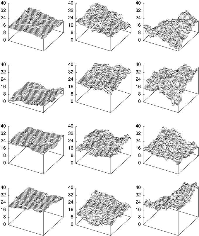
Figure 2. Fracture surfaces, showing the lower remaining part of a cube lattice of size L = 40 after it has broken completely. Four samples are included for D = 1 on the left, for D = 2 at center, and for D = −4 on the right.

3. Results and Discussion

In our calculations we have used open rather than periodic boundary conditions. This introduces edge effects, especially for small systems, but we assume it does not affect the roughness calculations significantly for our largest systems. For each trace along the surface we subtract the drift in the vertical direction, and overhangs which might appear are removed. The roughness is obtained as the root-mean-square of the variance perpendicular to the (average) fracture plane, i.e.,

$\begin{array}{cc}{W}_x(L)={\langle \frac{1}{L}{\displaystyle \sum _{i=1}^L{z}_x}{(i)}^2-{\left[\frac{1}{L}{\displaystyle \sum _{i=1}^L{z}_x}(i)\right]}^2\rangle }^{1/2},& (25)\end{array}$

where z_x(i) is the height in the vertical direction of the first intact node encountered when moving down toward the lower remaining part of the cube (those parts shown in Figure 2). Tracing parallel to the X-axis we obtain W_x, and parallel to the Y-axis we obtain W_y, results for W_x and W_y are statistically the same. We have evaluated four different disorders, having made three sets of calculations for type D > 0 disorder, i.e., D = 1, D = 2, and D = 4, and one set for type D < 0 disorder, i.e., D = −4. In each case a large number of samples were calculated for each size. The system sizes we show in the plots are from L = 3 up to L = 40 or L = 50, and for D = 1 we include L = 63.

In a log-log plot the self-affine relationship between the out-of-plane crack roughness W and the system size L shows up as a straight line, and we determine the roughness exponent from the slope of this line. Apart from the smallest systems, for which edge effects are significant, a self-affine relationship W ~ L^ζ emerges well within the range of system sizes included in the present study if we regard D = 2, D = 4, and D = −4. Presently system sizes for which we have a sufficiently large number of samples lie in the range L = 3 to about L = 50. Results for D = 2 and D = 4 are shown in Figures 3, 4, respectively. The exponent obtained for D = 2 is ζ = 0.62(2), based on a straight-line fit to systems L = 10, 13, 16, 19, 20, 22, 25, 32, and 40. For D = 4 we obtain ζ = 0.590(4), based on a straight-line fit to L = 10, 13, 16, 20, 25, 32, 40, and 50. At weak disorders the change in the fracture process from disorder dominated fracturing, where small cracks appear randomly throughout the material, to stress dominated fracturing, where a large crack emerges and breaks the sample, occurs at an early stage. Hence the computer time needed to break such each sample is less than that required to break a sample at strong disorder. Despite this, a very much larger number of samples is needed to obtain solid statistics at weak disorders. A comparable number of samples was generated for D = 2 and D = 4, but the statistics are stronger in the latter case.

FIGURE 3

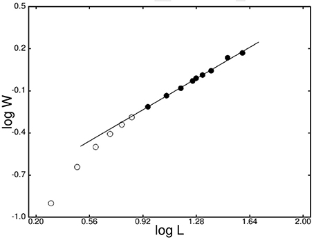
Figure 3. Logarithmic plot, showing the roughness, W, as a function of the system size, L, for disorder D = 2. Black circles denote those points to which the straight line, with slope ζ = 0.62(2), has been fitted. The largest errors on the points are approximately the size of the points.

FIGURE 4

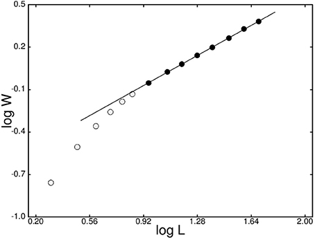
Figure 4. Logarithmic plot, showing the roughness, W, as a function of the system size, L, for disorder D = 4. Black circles denote those points to which the straight line, with slope ζ = 0.590(4), has been fitted. The errors on the points are smaller than the size of the points.

In the case of D = 1 it is perhaps more questionable whether a self-affine regime has appeared within the range of system sizes studied, as can be seen from Figure 5. In Figure 5 a line with slope ζ = 0.78 has been fitted to the values for L = 16, 20, 25, and 32, corresponding to an apparently linear regime. This is seen to cross over into a regime with a smaller roughness exponent. At present, however, we cannot tell what this exponent is, based on the system sizes used currently. For the number of samples calculated, the average values for L = 50 and L = 63 are subject to a certain amount of statistical fluctuation but these are not large enough to place them on the fitted slope. We assume that a self-affine regime manifests itself for larger system sizes.

FIGURE 5

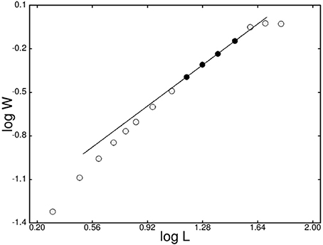
Figure 5. Logarithmic plot, showing the roughness, W, as a function of the system size, L, for disorder D = 1. Black circles denote those points to which the straight line, with slope ζ = 0.77(1), has been fitted. The errors on the points are larger than the size of the points, except for the largest system L = 63.

For weak disorders the fracture surface will appear as mainly flat plateaus, slightly stepped up or down in relation to each other, due to the surface height variations being smaller than the lattice course-graining. This effect is especially accentuated for small system sizes, but improves as system size increases. Because of this, the length scale at which the cross-over occurs decreases with increasing disorder and for this reason it appears that larger system sizes are required in order to reliably estimate the roughness exponent for weak disorders. So although D = 1 represents a comparatively strong disorder in two dimensions [24], where the resulting crack displays a very rough surface, this is not the case in three dimensions. In three dimensions the added constraint on the crack surface from the extra dimension causes the two dimensional traces along the three dimensional surface to be more smooth than what is the case for a trace along a purely two dimensional crack. Consequently, as can also be seen by examining the fracture surfaces shown in Figure 2, D = 1 in the threshold distribution corresponds to weak disorder in three dimensions. Hence, the inclusion of larger system sizes, with sufficiently many samples, is required to determine the exponent for D = 1 or weaker disorders.

We next consider fracture in the D < 0 regime. At weak disorder one has a more or less uniformly distributed strength throughout the elastic medium, interrupted here and there by the odd strong element. Fracture in this case is stress dominated from the onset—as the crack advances the next beams encountered along the path are most likely comparable in strength to those already broken and since the stress is highest at the crack tip these are the ones that will break next. Consequently, crack growth is localized and unstable from the beginning, resulting in a fracture surface that is quite smooth. As D increases, however, a region of stable crack growth emerges, since now the number of strong beams in the distribution of thresholds becomes significant. Fracture is now disorder dominated from the beginning and a rougher interface results as the randomly distributed micro-cracks gradually merge into a macroscopic fracture surface. Finally, at some point, fracture becomes unstable and the sample breaks completely. In studies of stress and strain in two dimensions, using a very large range of disorders [33], this turnover, from systems which are unstable from the onset to systems within which there is initially a complex coupled interaction between stress and disorder, is seen to occur for disorders approximately within the interval −2 < D < −3.

Presently, we include a single disorder for distributions with a tail toward strong elements, i.e., D = −4. The result obtained is ζ = 0.65(2), based on a straight-line fit to the average roughness values for L = 10, 13, 16, 20, 25, 32, and 40. This is shown in Figure 6, and the exponent is thus quite consistent with the results obtained for D > 0 distributions. With a given D expected to produce less roughness in three dimensions than in two dimensions, D = −4 here is probably close to this transient regime, where a controlled regime of micro-cracking appears. This could possibly account for the small difference obtained, i.e., ζ = 0.65 as opposed to ζ = 0.59–62 at high D > 0 disorders.

FIGURE 6

Figure 6. Logarithmic plot, showing the roughness, W, as a function of the system size, L, for disorder D = −4. Black circles denote those points to which the straight line, with slope ζ = 0.65(2), has been fitted. The largest errors for the black circles are comparable to the size of the symbols.

4. Conclusions

To summarize, a roughness exponent of approximately ζ ≃ 0.6 is obtained numerically for a discrete element model in the form of a cube lattice where forces are derived in analogy with elastic beams. Compared to other reported values in numerical works, this value is somewhat higher. One cannot really compare with results obtained in scalar models of fracture, such as the random fuse model, although the result is still in fair agreement with the various exponents obtained, i.e., 0.4 ≲ ζ ≲ 0.6, as reported in Batrouni and Hansen [9], Räisänen et al. [10], Räisänen et al. [11], Nukala et al. [12]. The Born model, which improves on the fuse model in that it includes elastic behavior, has yielded exponents in agreement with experiment, i.e., ζ ≃ 0.5 [20]. This model, as mentioned in the introduction is, however, not rotationally invariant.

The most relevant result with which to compare our current results are those of Nukala et al. [25], i.e., ζ ≃ 0.5. Our results are in fair agreement with this. A difference between the two studies is that in the former case periodic boundary conditions were used and also a slightly different fracture criterion. In two dimensions [24] we chose open boundary conditions to avoid having to address the problem of fitting a sine curve to the fracture surface. This because topologically the periodic lattice in two dimensions is a cylinder and the intersection of this with a plane is a sine curve. It may be difficult to judge whether a crack surface which appears to be a sine curve really is a sine curve or if this shape is something which appears as truly a part of the surface roughness. We chose to use open boundary conditions in three dimensions for similar reasons, and also generally to emulate a physical cube as it would appear in a fractured laboratory sample. To our knowledge, the significance of using different interaction formulae for combined loading is a subject which has not yet been investigated in studies using stochastic models. This is a subject which should be addressed in future studies.

Future studies should also address the issue of lattice topology. In two dimensions our calculations gave ζ = 0.86(3) [24] which is quite different from the two dimensional beam lattice result quoted in a study using a triangular lattice topology, i.e., ζ = 0.64(2) [34]. The triangular topology in two dimensions is actually required for a Cosserat medium (such as the beam lattice models) to be able to reproduce the macroscopic properties of a real elastic solid. In three dimensions, the cubic lattice topology is inadequate in this respect.

Conflict of Interest Statement

The authors declare that the research was conducted in the absence of any commercial or financial relationships that could be construed as a potential conflict of interest.

References

1. Mandelbrot BB, Passoja DE, Paullay AJ. Fractal character of fracture surfaces of metals. Nature (1984) 308:721. doi: 10.1038/308721a0

CrossRef Full Text | Google Scholar

2. Bouchaud E. Scaling properties of cracks. J Phys Condens Matter (1997) 9:4319. doi: 10.1088/0953-8984/9/21/002

CrossRef Full Text | Google Scholar

3. Herrmann HJ, Roux S. Statistical Models for the Fracture of Disordered Media. Amsterdam: North-Holland Publishing Company (1990).

Google Scholar

4. Alava MJ, Nukala PKVV, Zapperi S. Statistical models of fracture. Adv Phys. (2006) 55:349. doi: 10.1080/00018730300741518

CrossRef Full Text | Google Scholar

5. de Arcangelis L, Redner S, Herrmann HJ. A random fuse model for breaking processes. J Phys Lett. (1985) 46:L585. doi: 10.1051/jphyslet:019850046013058500

CrossRef Full Text | Google Scholar

6. Hansen A, Hinrichsen EL, Roux S. Roughness of crack interfaces. Phys Rev Lett. (1991a) 66:2476. doi: 10.1103/PhysRevLett.66.2476

Pubmed Abstract | Pubmed Full Text | CrossRef Full Text | Google Scholar

7. Bakke JØH, Bjelland J, Ramstad T, Stranden T, Hansen A, Schmittbuhl J. Roughness of brittle fractures as a correlated percolation problem. Phys Scripta (2003) T106:65. doi: 10.1238/Physica.Topical.106a00065

CrossRef Full Text | Google Scholar

8. Zapperi S, Nukala PKVV, Šimunović S. Crack roughness and avalanche precursors in the random fuse model. Phys Rev E (2005) 71:026106. doi: 10.1103/PhysRevE.71.026106

Pubmed Abstract | Pubmed Full Text | CrossRef Full Text | Google Scholar

9. Batrouni GG, Hansen A. Fracture in three-dimensional fuse networks Phys Rev Lett. (1998) 80:325. doi: 10.1103/PhysRevLett.80.325

Pubmed Abstract | Pubmed Full Text | CrossRef Full Text | Google Scholar

10. Räisänen VI, Alava MJ, Nieminen RM. Fracture of three-dimensional fuse networks with quenched disorder. Phys Rev B (1998a) 58:14288. doi: 10.1103/PhysRevB.58.14288

CrossRef Full Text | Google Scholar

11. Räisänen VI, Seppälä ET, Alava MJ, Duxbury PM. Quasistatic cracks and minimal energy surfaces Phys Rev Lett. (1998b) 80:329. doi: 10.1103/PhysRevLett.80.329

CrossRef Full Text | Google Scholar

12. Nukala PKVV, Zapperi S, Šimunović S. Crack surface roughness in three-dimensional random fuse networks. Phys Rev E (2006) 74:026105. doi: 10.1103/PhysRevE.74.026105

Pubmed Abstract | Pubmed Full Text | CrossRef Full Text | Google Scholar

13. Daguier P, Henaux S, Bouchaud E, Creuzet F. Quantitative analysis of a fracture surface by atomic force microscopy. Phys Rev E (1996) 53:5637. doi: 10.1103/PhysRevE.53.5637

Pubmed Abstract | Pubmed Full Text | CrossRef Full Text | Google Scholar

14. Daguier P, Nghiem B, Bouchaud E, Creuzet F. Pinning and depinning of crack fronts in heterogeneous materials. Phys Rev Lett. (1997) 78:1062. doi: 10.1103/PhysRevLett.78.1062

CrossRef Full Text | Google Scholar

15. Milman VY, Blumenfeld R, Stelmashenko NA, Ball RC. Comment on “Experimental measurements of the roughness of brittle cracks.” Phys Rev Lett. (1993) 71:204. doi: 10.1103/PhysRevLett.71.204

Pubmed Abstract | Pubmed Full Text | CrossRef Full Text | Google Scholar

16. Boffa JM, Allain C, Hulin J. Experimental analysis of fracture rugosity in granular and compact rocks. Eur Phys J. (1998) 2:281.

Google Scholar

17. Ponson L, Auradou H, Pessel M, Lazarus V, Hulin JP. Failure mechanisms and surface roughness statistics of fractured Fontainebleau sandstone. Phys Rev E (2007) 76:036108. doi: 10.1103/PhysRevE.76.036108

Pubmed Abstract | Pubmed Full Text | CrossRef Full Text | Google Scholar

18. Bohm M, Huang K. Dynamical Theory of Crystal Lattices. New York, NY: Oxford University Press (1954).

19. Caldarelli G, Cafiero R, Gabrielli A. Dynamics of fractures in quenched disordered media. Phys Rev E (1998) 57:3878. doi: 10.1103/PhysRevE.57.3878

CrossRef Full Text | Google Scholar

20. Parisi A, Caldarelli G, Pietronero L. Roughness of fracture surfaces. Europhys Lett. (2000) 52:304. doi: 10.1209/epl/i2000-00439-9

CrossRef Full Text | Google Scholar

21. Feng S, Sen PN. Percolation on elastic networks: new exponent and threshold. Phys Rev Lett. (1984) 52:216. doi: 10.1103/PhysRevLett.52.216

Pubmed Abstract | Pubmed Full Text | CrossRef Full Text | Google Scholar

22. Roux S, Guyon E. Mechanical percolation: a small beam lattice study, J Phys Lett. (1985) 46:L999. doi: 10.1051/jphyslet:019850046021099900

CrossRef Full Text | Google Scholar

23. Herrmann HJ, Hansen A, Roux S. Fracture of disordered, elastic lattices in two dimensions. Phys Rev B (1989) 39:637. doi: 10.1103/PhysRevB.39.637

Pubmed Abstract | Pubmed Full Text | CrossRef Full Text | Google Scholar

24. Skjetne B, Helle T, Hansen A. Roughness of crack interfaces in two-dimensional beam lattices, Phys Rev Lett. (2001) 87:125503. doi: 10.1103/PhysRevLett.87.125503

Pubmed Abstract | Pubmed Full Text | CrossRef Full Text | Google Scholar

25. Nukala PKVV, Barai P, Zapperi S, Alava MJ, Šimunović S. Fracture roughness in three-dimensional beam lattice systems. Phys Rev E (2010) 82:026103. doi: 10.1103/PhysRevE.82.026103

Pubmed Abstract | Pubmed Full Text | CrossRef Full Text | Google Scholar

26. Roark RJ, Young WC. Formulas for Stress and Strain. New York, NY: McGraw-Hill Book Company (1975).

Google Scholar

27. Crandall SH, Dahl NC An Introduction to the Mechanics of Solids. New York, NY: McGraw-Hill Book Company (1959).

Google Scholar

28. Hestenes MR, Stiefel E. Methods of conjugate gradients for solving linear systems. Nat Bur Stand J Res. (1952) 49:409. doi: 10.6028/jres.049.044

CrossRef Full Text | Google Scholar

29. Press WH, Teukolsky SA, Vetterling WT, Flannery BP. Numerical Recipes in Fortran 77. New York, NY: Cambridge University Press (1992).

Google Scholar

30. Roux S, Hansen A. Off-threshold multifractality in percolation. Europhys Lett. (1989) 8:729. doi: 10.1209/0295-5075/8/8/004

CrossRef Full Text | Google Scholar

31. Roux S, Hansen A. Early stages of rupture of disordered materials. Europhys Lett. (1990) 11:37. doi: 10.1209/0295-5075/11/1/007

CrossRef Full Text | Google Scholar

32. Hansen A, Hinrichsen EL, Roux S. Scale-invariant disorder in fracture and related breakdown phenomena. Phys Rev B (1991b) 43:665. doi: 10.1103/PhysRevB.43.665

Pubmed Abstract | Pubmed Full Text | CrossRef Full Text | Google Scholar

33. Skjetne B, Helle T, Hansen A. Scaling behaviour of damage in the fracture of two-dimensional elastic beam lattices. Europhys Lett. (2007) 80:28002. doi: 10.1209/0295-5075/80/28002

CrossRef Full Text | Google Scholar

34. Nukala PKVV, Zapperi S, Alava MJ, Šimunović S. Crack roughness in the two-dimensional random threshold beam model. Phys Rev E (2008) 78:046105. doi: 10.1103/PhysRevE.78.046105

Pubmed Abstract | Pubmed Full Text | CrossRef Full Text | Google Scholar