Analysis of image vs. position, scale and direction reveals pattern texture anisotropy

1. Introduction

Inhomogeneous systems require specific tools for their quantification, whether for data analysis, or comparison with numerical and analytical modeling. Analysis of patterns to extract relevant physical information is a fruitful approach in a wide range of systems [1]. It strongly depends on the type of pattern. Patterns made of well-defined individual units such as biological tissues, grains in polycrystals, foams and emulsions, display immediately accessible information; they can be described by specific tools which take into account their topology (e.g., connections between individual objects) [2]. Patterns in which identifiable individual objects are present at several different scales, such as transport or telecommunication networks, fiber bundles or polymer gels, may reveal more information under a multiscale analysis. Finally, patterns which involve several scales and objects too intricated to be separately identified, ranging from stars and galaxies to colloidal materials, diphasic systems and porous media, can rather be statistically characterized, for instance by their texture [3].

Even in these latter class of less obviously decomposable patterns, it is important to determine the local anisotropy, for instance in nuclear magnetic resonance images (MRI) of brain [4]. For fractures patterns, tools exist to characterize their structure, heterogeneity, topology and correlations [5]. However, in addition, preferential directions are clearly visible by eye: they depend on both scale and position (Figure 1). It is important to make this observation quantitative, especially since mechanical descriptions often require to take into account directions, for instance of principal stresses and strains. Several good methods already exist to quantitatively reveal and characterize the local anisotropy. Our goal is to complement them by providing a method which: (i) cumulates analysis in terms of position, direction and scale; (ii) applies to a set of patterns as general as possible; (iii) is simple and fast to understand, implement, execute and exploit.

FIGURE 1

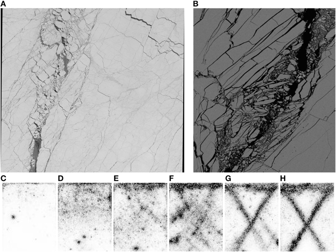
Figure 1. Fracture patterns. (A) Arctic sea ice cover; image size: 60 km. (B) Granite thin section: a sample of height 80 mm and diameter 40 mm is deformed until rupture and the fracture is sheared over 2 mm. Image size: 4 × 3 mm², i.e., 1024 × 888 pixels of 3.9 μm. (C–H) Granular material: maps of correlation of the scattered light. White pixels correspond to high correlation (i.e., weak deformations) and black pixels to low correlation (i.e., large deformation). The size of one pixel corresponds to ≈ 0.65 mm (2.6 grain diameters). Deformations are 0.9% (C), 1.6% (D), 3.3% (E), 5.7% (F), 8.3% (G), and 9.5% (H). For details, see Sections 3.1.1, 3.2.1, 3.3.1, respectively.

The outline of this paper is as follows. Section 2 exposes the principle of the method. Section 3 applies it to three experimental examples. Section 4 compares this method with existing ones. Section 5 concludes. The “Supplementary Material” presents various tests of measurement robustness.

2. Method Outline

At each step of the proposed method, the users can select variants and validation criteria according to their own scientific requirements, their practical applications, and the features of interest in the patterns they study. These choices are not necessarily based on a mathematical justification and should not be validated using visual detection only.

2.1. Images

2.1.1. Input data

An image is a signal, encoded through pixels, each pixel position $\overrightarrow{M}$ having integer coordinates.

The pixels constitute an array, usually in two or three-dimensions. It can be in any higher dimension, for instance for series of images depending on parameters, like a movie. For simplicity of explanations and especially of representation, examples below are in 2D, but the formalism is indifferent to the dimension.

The information is any physical quantity I($\overrightarrow{M}$), that is, a field defined over the pixels. In examples below, I is a binary number, 0 or 1, or a gray level, an integer number for instance between 0 and 255. The formalism generalizes to I being a positive scalar, that is a continuous gray level; a vector with three positive components, such as RGB images; or even a higher order tensor.

2.1.2. Pre-processing

Only few, basic image pre-processing steps are required.

Without loss of generality, we consider a signal to be analyzed which is coded in white (large I), over a black (low I) background. Otherwise, a symmetry transform should be applied to the image before starting the analysis: I → 1 − I for a binary image, I → 255 − I for a gray level image.

It is useful to eliminate isolated white pixels using a slight filtering of the image, such as opening (erosion-dilatation), median filter or low pass filter.

A gray level image can be used as it is, I = 0 to 255; or first thresholded, I = S to 255, where the threshold S is selected according to the noise level and the signal considered to be relevant; or binarized, I = 0 or 1, where 1 represents the signal and 0 the background.

In the examples below, analysing binarized image yields qualitatively the same results (orientation and scale of maximal anisotropy) as analysing gray level images, and quantitatively the signal to noise ratio is larger (data not shown), while the validation of the results by visual observation of the image is much easier.

2.2. Formalism

2.2.1. Boxes

We introduce a scale ℓ, and a list of positions $\overrightarrow{r}$ inside the image; $\overrightarrow{r}$ does not need to coincide exactly with a pixel position (its coordinates need not be integers).

Consider any function f($\overrightarrow{M}$) defined over the image $\overrightarrow{M}$. The approximation of f at scale ℓ, noted $\tilde{f}$($\overrightarrow{r}$, ℓ) defined as the value of f over an analyzing box at scale ℓ, centered at $\overrightarrow{r}$, is:

$\begin{array}{cc}\tilde{f}(\overrightarrow{r},\ell )={\displaystyle \sum _{\overrightarrow{M}}\varphi }\left(\frac{\overrightarrow{M}-\overrightarrow{r}}{\ell }\right)f\left(\overrightarrow{M}\right)& \left(1\right)\end{array}$

where ϕ is a smoothing function with compact support, which defines the analysis box.

The box can be a circle of center $\overrightarrow{r}$ and radius ℓ, or a a square of center $\overrightarrow{r}$ and side 2ℓ. The sum ${\displaystyle {\sum }_{\overrightarrow{M}}\varphi f}$ over all pixels in the analysis box is then denoted ∑_boxf. The box centers $\overrightarrow{r}$ can for instance be placed at each pixel of the image (sliding boxes) or at each node of a larger grid.

Some boxes overlap image boundaries, and are thus incomplete. There are various possibilities to deal with them, which can be selected according to the image. First, one can ignore these incomplete boxes in the analysis. Second, one can add as many black pixels as necessary to complete them without artificial signal. Third, one can put artificial periodic boundary conditions, and complete them with pixels coming from the opposite side of the image. Fourth, one can make the outer boxes coincide with the image edges: then if the image size is not a multiple of the box size, in order to tile the whole image the boxes should have variables overlaps.

2.2.2. Inertia tensor

Setting now f ≡ I in Equation (1), we define the signal intensity in the box at the chosen scale ℓ as:

$\begin{array}{cc}\tilde{I}\left(\overrightarrow{r},\ell \right)={\displaystyle \sum _{\overrightarrow{M}}\varphi }I\left(\overrightarrow{M}\right)={\displaystyle \sum _{\text{box}}I}.& \left(2\right)\end{array}$

If $\tilde{I}$($\overrightarrow{r}$, ℓ) = 0 we stop the analysis for the corresponding box. Otherwise, we define the signal barycenter $\overrightarrow{G}$ within the box by setting f ≡ I$\overrightarrow{M}$ in the Equation (1), for the numerator:

$\begin{array}{cc}\overrightarrow{G}=\frac{1}{\tilde{I}\left(\overrightarrow{r},\ell \right)}{\displaystyle \sum _{\overrightarrow{M}}\varphi }I\left(\overrightarrow{M}\right)\overrightarrow{M}=\frac{{\displaystyle {\sum }_{\text{box}}I}\overrightarrow{M}}{{\displaystyle {\sum }_{\text{box}}I}}.& \left(3\right)\end{array}$

We then measure the inertia tensor of the signal within the box, taken at the barycenter G, through:

$\begin{array}{cc}\overline{\overline{P}}\left(\overrightarrow{r},\ell \right)={\displaystyle \sum _{\overrightarrow{M}}\varphi }I\left(\overrightarrow{M}\right)\overrightarrow{GM}\otimes \overrightarrow{GM}.& \left(4\right)\end{array}$

In Equation (4), the center $\overrightarrow{r}$ of the analysing box should be distinguished from the barycenter G of the signal in this box. By construction, $\overline{\overline{P}}$ is a symmetric tensor. In 2D, it writes:

$\begin{array}{cc}\overline{\overline{P}}\left(\overrightarrow{r},\ell \right)={\displaystyle \sum _{\text{box}}\left(\begin{array}{cc}{X}^2& XY\\ XY& Y^2\end{array}\right)I,}& \left(5\right)\end{array}$

where (X, Y) are the coordinates of $\overrightarrow{GM}$.

2.2.3. Some variants

Equation (5) admits several variants.

I could be a vector or a higher rank tensor. Correspondingly, $\overline{\overline{P}}$ would be a tensor which rank is the rank of I plus two.

To give the same weight to pixels close to the barycenter and close to the box boundary, one can set f ≡ I / |$\overrightarrow{GM}$|² in Equation (1) and define the direction tensor:

$\begin{array}{cc}\begin{array}{l}\overline{\overline{Q}}\left(\overrightarrow{r},\ell \right)={\displaystyle \sum _{\overrightarrow{M}}\varphi }\frac{I\left(\overrightarrow{M}\right)}{|\overrightarrow{GM}{|}^2}\overrightarrow{GM}\otimes \overrightarrow{GM}\\ ={\displaystyle \sum _{\text{box}}\frac{1}{X^2+Y^2}}\left(\begin{array}{cc}{X}^2& XY\\ XY& Y^2\end{array}\right)I.\end{array}& \left(6\right)\end{array}$

By definition, $\overline{\overline{Q}}$ depends on cos²θ, cosθ sin θ et sin²θ, and so on 2θ, where θ is the angle between $\overrightarrow{GM}$ and the x axis. Note that since the denominator of Equation (6) can vanish for M = G, it is reasonable to introduce a cut-off and sum only over the pixels that are at least 1 pixel away from the barycenter G. Comparing Equation (2) with Equation (6) shows that the trace of the direction tensor is:

$\begin{array}{cc}\text{Tr }\overline{\overline{Q}}\left(\overrightarrow{r},\ell \right)={\displaystyle \sum _{\text{box}}I}=\tilde{I}\left(\overrightarrow{r},\ell \right).& \left(7\right)\end{array}$

The choice between $\overline{\overline{P}}$ and $\overline{\overline{Q}}$ does not introduce any qualitative difference. In some boxes the result can be quantitatively different, but after averaging over boxes, both yield similar statistical results. $\overline{\overline{Q}}$ is more sensitive to the directions close to the box center, $\overline{\overline{P}}$ is more robust to noise and reflects better the directions at the box scale. This test, as well as other tests of robustness with respect to variants (binarization, box shape, box position) and to noise, is presented in the “Supplementary Material.”

2.3. Measurements and Representations

Different measurements can be performed. Their dependence with scale, position and orientation can be quantitatively represented using for instance graphs, maps and polar plots, respectively. In 3D images, measurements are similar as in 2D, but representations are less legible.

2.3.1. Graphs

Graphs can evidence the quantitative aspects of the dependence with scale.

First, the scale is fixed. For each box, the inertia tensor is measured. Since it is symmetric, it can be diagonalized, and has two real eigenvalues λ₁ > λ₂ ≥ 0. Its anisotropy 1 − λ₂/λ₁ calculated. Then the anisotropies of each (non-empty) box are averaged and their standard deviation recorded. Repeating this measurement at different scales yields a graph of the average anisotropy 〈 1 − λ₂/λ₁ 〉 vs. scale, plotted with bars reflecting the spatial variations of the anisotropy values.

An artificial example is shown in insert of Figure 2. The structure is a cross loosely following the diagonals of a square. The main part of Figure 2 shows the average of the anisotropy vs. scale. As expected, it displays a maximum at the scale where the eye notes the maximal anisotropy. For small enough scales the main pattern contained in a box is a part of one of the diagonals, so that the anisotropy is high, and increases with the scale. For a size of 128 or 256 pixels, which correspond to 1/8th and one quarter of the image, the pattern contains one diagonal and the anisotropy is maximal. For the larger scale, due to its symmetry, the whole pattern is globally isotropic, the anisotropy curve drops almost to zero. In cases where it would be important to distinguish a cross from a uniform image, one should adapt Equation (5) to characterize a quadrupolar rather than dipolar anisotropy.

FIGURE 2

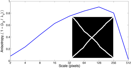
Figure 2. Example of a synthetic image and its analysis. In insert : artificial image (512 × 512 pixels) consisting in a cross loosely following the diagonals of a square. The lines are about 11 pixels wide. The main graph represents the anisotropy as a function of the scale.

An alternative measurement is performed as follows. The tensor in each box is calculated, then all these tensors are averaged, and the resulting average tensor is diagonalized. This determines the anisotropy of the average tensor, which is a single tensor per image. At the largest scale where there is a single box as large as the image, this measurement coincides with the preceding one. However, it is usually much smaller than the average of each tensor's anisotropy, especially when the average tensor takes into account contributions in various directions. In that case, each box has a strong anisotropy, so that the average of anisotropies is large, but since boxes have various directions, the average tensor is globally isotropic, hence its anisotropy is very low. This is called the “powder effect” in crystallography, where different anisotropic grains together contribute to an isotropic signal. Such graph is useful to emphasize the appearance of correlated anisotropy at large scale.

2.3.2. Maps

Maps evidence qualitative features of the spatial variations.

At a given scale, in each box (and thus at each position) the inertia tensor is measured. No average is performed. Each tensor is diagonalized. In each box, the anisotropy or direction can be separately represented, for instance as a color map. Or they can be represented together, using the classical representation of the inertia tensor as an ellipse, with axis lengths λ₁ and λ₂ in the directions corresponding to their respective eigenvectors¹ : the map is then a juxtaposition of different ellipses.

One can rescale each ellipse by inscribing it in a square of the same size as the box where it is measured. Thus, the ellipse size reflects the scale of measurement. For a map constructed at a given scale, all ellipses have a comparable size. There could be an alternative possibility, where each ellipse size is proportional to the intensity of the signal within the box.

At each position, several ellipses measured at different scales can be superimposed. In order to keep some legibility, it is possible to represent only the eigenvectors rather than the whole ellipses. Or to plot the same number of ellipses at all scales (which means removing several boxes at small scales). Figure 3A shows an example for an artificial pattern with two well-defined length scales. At small scale, the ellipse is aligned with each small structures, while at large scale the ellipse reflects the global arrangement of the pattern.

FIGURE 3

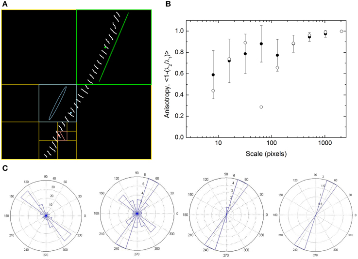
Figure 3. Two artificially separated length scales. (A) Synthetic image with two well-defined anisotropy length scales. Inertia tensor in three boxes, each at a different scale, is represented using superimposed ellipses. Colored points label the barycenter of the signal. Image side : 2048 pixels. Box size : pink 128, blue 512, green 1024 pixels. (B) Anisotropy graph. Closed circles: average anisotropy 1-λ₂/λ₁ measured on (A), here using circular boxes. Bars: standard deviation. Open circles: anisotropy of the average tensor. (C) Orientation roses. Measurements are performed on circular boxes with diameters (from left to right): 64, 128, 512, and 1024 pixels. The transition is mainly between 64 and 128 pixels. At 1024 pixels, the average is performed only over four boxes.

A map can become more illuminating when superimposed on the initial image (Figure 3A) or combined with a quantitative graph: in Figure 3B, the transition region between both length scales is visible around 64–128 pixels, especially for the anisotropy of the average tensor, which evidences an effective correlation scale for the anisotropy.

2.3.3. Polar plots

Roses are quantitative representations that focus on the dependence with orientation, rather than the anisotropy itself.

For a given scale, in each box (that is, at each position) the inertia tensor is measured. It is diagonalized and only the direction θ of the eigenvector associated with its main eigenvalue λ₁ is recorded. The histogram of θ is represented: since for an eigenvector θ and θ + π play the same role, they are both plotted simultaneously. The same measurement can be repeated at different scales: in Figure 3C, the change in the principal direction is clearly visible at 128 pixels, where many non-empty boxes contain only a tiny amount of signal.

3. Results

Examples are fracture patterns in ice, granite thin sections, granular medium (Figure 1). Unless specified, all measurements presented below are performed in square boxes.

3.1. Sea Ice Fracturing

3.1.1. Data

The image analyzed is a visible wavelength satellite photograph of the Arctic sea ice cover, taken by “Système Pour l'Observation de la Terre” (SPOT) in early spring on April 6th, 1996, centered around 80°11′N, 108°33′W (Figure 1A). It contains 5977 × 5977 pixels, each pixel being 10 m, i.e., the image covers about 60 × 60 km². The thickness ~ 1 − 3 m of the sea ice cover is much smaller than the lateral extension of the image. Due to this aspect ratio, the ice sheet can be considered as two-dimensional.

Owing to the much stronger albedo of snow-covered sea ice (>0.6) compared to open ocean (<0.2) [6], newly opened fractures appear much darker than the surrounding sea ice. This is clearly visible on the gray-level (I_g) histogram (Figure 4A) of the image where ice values are centered around I_g = 140. The gray-levels result from several physical independent factors (sea ice vs open water, but also local roughness of the surface, type of snow, …) and from measurement noise. The different secondary peaks observed below I_g = 125 may correspond to different levels of (recent) refreezing stages, from purely open water to thin, snow-free ice. In the sea ice terminology, these fractures are called “leads.” They differ in nature and origin from the so-called “polynya” which are open water areas inside the ice pack resulting from warm water upwelling or wind-induced drift away from a fixed boundary; there is no polynya in Figure 1A. This albedo difference can be used to convert this grayscale image to a binary image of only fractures or ice, as done in Weiss and Marsan [7] and Marcq and Weiss [8].

FIGURE 4

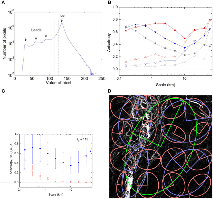
Figure 4. Analysis of the sea ice image (Figure 1A). (A) Gray-level histogram of the raw image. The dashed vertical lines indicate the range of threshold values used for binarization. (B) Anisotropy vs. scale, for different values of the threshold. Solid lines, closed symbols: anisotropy (averaged over all boxes) vs scale for binary images obtained from different thresholds (red upward triangles: I_th = 95, blue downward triangles: I_th = 115, gray circles: I_th = 125). Dashed lines, open symbols: anisotropy of the average tensor, same symbol and color code. (C) Test of significance. Blue triangles: anisotropy vs scale for I_th = 115 [same data as in (B)]. Errors bars correspond to the standard deviation over the different boxes of the same size. Red open circles: same measurement on a random image of the same size, with the same proportion of black pixels: in this case, as expected, the anisotropy is zero at large scales, but increases toward small scales as the result of pixelation (see text for details). (D) Anisotropy ellipses, drawn at scales of whole (green), half (purple) and quarter (pink) of image width.

The fracture network is typical of winter pack ice and has been already analyzed in terms of fracture density and associated scaling properties [7]. It was shown that this network defines an ensemble of ice fragments (“floes”) power-law distributed in size, whereas the fracture density is characterized by multifractal properties, both observations arguing for the scale invariant character of sea ice fracturing [7, 9]. In these previous analyses, the anisotropy of the fracture pattern was not considered.

3.1.2. Analysis

At the scale of an individual fracture, the anisotropy arises from fracture mechanics: the average fracture opening is much smaller than the fracture length (see Figure 1A). We now ask whether this anisotropy is preserved for fracture networks, and whether it depends on the spatial scale.

Figure 4B shows the anisotropy 〈 1 − λ₂/λ₁ 〉 vs. scale for binary images obtained from the grayscale image of Figure 1A using different thresholds, I_th = 95, 115, 125. For gray levels I_g ≤ I_th, a binary value I_b = 1 is assigned to the image (water), and I_b = 0 instead (ice). No additional image processing was performed on the raw grayscale image. Two anisotropy measures are shown at each scale: the index averaged over all square boxes covering the image at a given scale, 〈 1 − λ₂/λ₁ 〉 (closed symbols), and the index of the averaged tensor (open symbols). These averages are performed on non-empty boxes, but without additional weighting based on the total intensity contained in the box.

A similar analysis performed on the raw grayscale image (not shown) leads to a similar evolution with scale, but very small anisotropies. This is mainly due to (i) the reinforcement of contrast induced by binarization, and (ii) the fact that the averages are performed in this case over all boxes, including many “ice-only” or “water-only” boxes over which the gray-level results from noise or processes not related to fracturing.

The evolution of the averaged index 〈 1 − λ₂/λ₁ 〉 is qualitatively similar whatever the threshold I_th: a maximum anisotropy at the scale of the entire image (5977 pixels, ~60 km), a minimum observed at ~10 km (1024 pixels), and an increase toward smaller scales. Anisotropies are larger for lower thresholds I_th. This might indicate that a part of noise not related to fracturing is included in the binary image when using a threshold too close to the gray-level histogram maximum (I_g = 140) corresponding to ice (Figure 4A).

On the other hand, this example also illustrates the intrinsic limitations of anisotropy measurements at small scales as the result of pixellisation. Figure 4C shows the averaged index 〈 1 − λ₂/λ₁ 〉 calculated for a spatially randomly reshuffled version of the sea ice image binarized with I_th = 115. The resulting image contains the same number of non-empty (I_b = 1) pixels as the original binary image, though randomly distributed in space, i.e., without expected anisotropy. The associated anisotropy is indeed negligible above 1 km (128 pixels), but becomes non-negligible compared to the averaged index of the original image for L = 32 pixels (320 m) and below. This can be easily understood by the possibility to obtain by chance an anisotropic distribution of filled pixels for such small boxes.

The large anisotropy obtained at the image scale (60 km) is clearly the signature of the large faulting system crossing the left part of the image, with fragmented material inside. This is confirmed by the corresponding ellipse inclined at about 60° (Figure 4D). Large values obtained below ~2 km probably correspond to the strong anisotropy of the narrow fractures observed on both sides of this system. These small scales fractures may have different orientations, thus explaining that the anisotropy of the averaged tensor is small below 10 km: in other words, the correlation length associated to the orientation of this secondary fracturing network is small; L = 10 km appears as a transition scale between two fracturing systems, at least in terms of anisotropy.

Figure 4D shows the ellipses constructed at this scale, which eccentricity is indeed, in average, much reduced compared to the ellipse corresponding to the global scale. Such transition scale was not observed in terms of fracture density, which is characterized by multifractal, i.e., scale invariant, properties [7]. Obviously, a much more comprehensive analysis of sea ice fracturing networks from various images covering a wide range of spatial scales would be needed to conclude on the ubiquitous (or not) character of such transition scale for sea ice fracturing anisotropy. The present analysis simply demonstrates the ability of our methodology to reveal the anisotropy of fracture patterns at different scales, with minimal pre-processing of the raw image (simple binarization).

3.2. Thin Sections of Granite

3.2.1. Data

Figure 1B shows fractures in compressed granite [10]. The rock is compressed in laboratory, enough for allowing cracks to develop. At the onset of damage, their direction of propagation is parallel to the direction of major stress which induces a strong damage anisotropy. Beyond a given threshold of crack density, the damage becomes localized along shear bands characterized by a concentration of cracks which produces a granular material which geometry is conditioned by the orientation of cracks and the amount of deformation. At this stage a strong anisotropy of the grain shape is expected. Deformation then develops mainly within the granular material; grains fragment, becoming more and more isotropic.

At the end of the experiment, epoxy resin is injected in the sample to preserve its structure during machining of a thin section. The images are obtained by scanning electron microscopy where gray levels reflect the atomic mass. The resin appears in black, so that cracks and grain boundaries are easy to identify. The analysis of the anisotropy should identify areas that experienced strong deformation (more isotropic) and also a progression from damaged areas (anisotropic) to granular areas (less anisotropic when approaching of the area of high deformation).

3.2.2. Analysis

Figure 1B was analyzed like sea ice (Section 3.1.2). The contrast between the non-fractured granite (I_g around 120) and the resin/fractures (I_g close to 0) is excellent, thus making the binarization straightforward. Consequently, the anisotropy measurements weakly depend on the selected threshold I_th. The results presented in Figure 5 were obtained for I_th = 50 and do not change for I_th = 30 or 70.

FIGURE 5

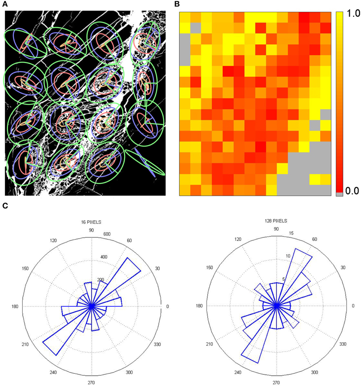
Figure 5. Analysis of granite (Figure 1B). (A) Analysis in position, orientation and scale. There are 4 × 4 analysis boxes placed on a grid of 110 pixels step centered on the image. Concentric ellipses represent measurements at 32 (orange), 64 (red), 96 (blue), 128 pixels (green). (B) Map of the anisotropy index 〈 1 − λ₂/λ₁ 〉 at scale 64 pixels. Red: weak anisotropy; yellow: strong anisotropy; gray; boxes without information. (C) Roses: 16 pixels (left) and 128 pixels (right). Threshold = 50, squared boxes (circular boxes yield indistinguishable results).

Figure 5A shows the ellipses constructed at different scales (from 32 to 128 pixels) and centered at different positions. Along the main inclined fault containing fragmented material, the anisotropy is small at scale 64 pixels, illustrating the relative isotropy of the highly fragmented gouge. It slowly increases toward larger scales, probably as a result of partial sampling of the anisotropy of the fault itself. Fractured zones on both sides of the main fault show very strong anisotropies at small scales associated to single elongated fractures, as well as sharp rotations of principal directions when several fractures are included within the box. This distinction between a fault with fragmented gouge, surrounded by zones of intense fracturing without fragmentation, was also observed on the sea ice image (Figure 1A), for spatial scales 7 orders of magnitude larger.

Figure 5B shows a colored map of the anisotropy index 〈 1 − λ₂/λ₁ 〉 calculated at the scale L = 64 pixels (gray boxes correspond to empty boxes). This shows quantitatively the gradient of anisotropy from the gouge material inside the fault to the much more anisotropic peripheral fractured zones. This result highlights the differences between fracture and fragmentation processes: while fractures are initiated locally under tension (mode I) with opening much smaller than fracture length, i.e., characterized by a strong anisotropy, fragmentation under shear is a complex multiscale process involving friction, grain rotation and comminution (e.g., [11–14]) that leads to relatively isotropic grain shapes. The present analysis clearly reveals this transition from one mechanism to another across the fault plane.

This space analysis quantifies what the eye detects qualitatively. It can be complemented by an angle analysis, which clearly identifies the main directions of anisotropy (Figure 5C). The scale analysis is similar to Figure 4B, but less pronounced, and with a minimum around 100–200 pixels (data not shown).

3.2.3. Simulations

We also analyse numerical simulations of progressive damage: for details see Ref. Amitrano [15]. Briefly, a finite element model is progressively loaded in order to increase the stress supported by the material. The strength of each element is choosen at random. To mimic the effect of increasing crack density, when the stress in a element reaches its strength, its elastic modulus is decreased by a constant factor less than unity. A model on a 256 × 128 grid is plotted here as a corresponding 512 × 256 pixels image, so each grid unit is covered by 4 pixels.

The diffuse and isotropic damage progressively evolves toward localized and anisotropic damage. Due to elastic interactions, the damage becomes progressively localized until the rupture of the whole sample, like in natural materials (Figure 1B). The damage parameter is D = 1 − E/E₀, where E is the current elastic modulus and E₀ is the initial elastic modulus. Figures 6A–C show the increments in damage D at three of the last steps, during damage localization.

FIGURE 6

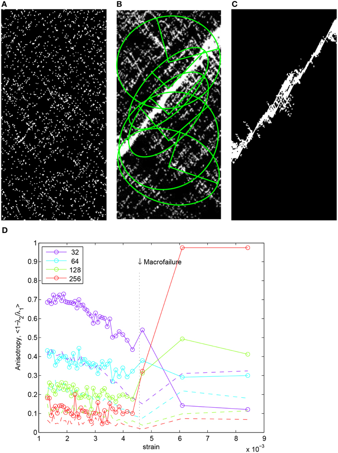
Figure 6. Simulations of progressive damage in granite compression. (A–C) Snapshots of the incremental damage. The cells that experienced damage during the step appear in white and the others in black. The whole simulation is decomposed in 40 steps of incremental damage, each step corresponding to an equal number of damage events. (A) Step 34, (B) step 38, (C) step 39. On (B), anisotropy ellipses at image width are superimposed. (D) Mean anisotropy at different scales (32, 64, 128, 256 pixels) for each strain step. Steps are spaced in order to ensure an equal number of damage events in each step. Dotted lines correspond to the same damage distribution but spatially spread at random.

Figure 6B shows the ellipse analysis for step 38 and Figure 6D shows the mean anisotropy at different scales for all the steps. To detect possible biases related to changes in damage intensity, we also performed the analysis for the same damage distribution but spatially spread at random (dotted lines in Figure 6D). The pattern of anisotropy can be considered to be significant as a clear departure from random images exists (except for largest scale in the initial steps). The anisotropy evolves toward the macro-failure with a clear dependence on scale. Anisotropy progressively decreases for small scales (32 pixels) whereas for large scale it increases suddenly when the macrofailure occurs. The intermediate scale of 64 pixel shows no particular trend and appears as a transition scale.

3.3. Granular Material

3.3.1. Data

Mohr-Coulomb analysis predicts that failure in granular material occurs along surfaces where the ratio of tangential stress over normal stress attains a material dependent ratio, called internal friction coefficient [16]. However, mechanisms of plasticity of disordered material suggest that preferential orientations for deformations are related to the stress redistribution after localized deformations (directions of the Eshelby stress tensor [17]) which are given by elastic properties and geometry of localized deformations. The determination of the anisotropy at different scales may allow to see the competition between those two failure mechanisms.

Ref. Le Bouil et al. [18] designed an experiment in order to look at the precursors of failure. Briefly, a granular material composed of glass beads of diameter d = 0.25 mm is placed between a latex membrane and a transparent glass plate. A confining pressure −σ_xx is applied laterally along the horizontal axis x, and the material is compressed slowly in the perpendicular direction z, with a pressure −σ_zz. The granular material is illuminated with a laser light, and the scattered light detected with a camera. The coherence of the scattered light is measured with a normalized correlation function which is 1 if no deformation takes places, and which is lower than 1 when deformation takes place [19, 20].

The map of the scattered light correlation between successive images is calculated (Figures 1C–H). It shows an evolution of the correlation of the scattered intensity between two successive images acquired at the global axial deformations ε = ΔL/L and ε + Δε with Δε ≈ 1 × 10⁻⁵.

White pixels correspond to well-correlated scattered light (i.e., weak deformation of the material), and gray pixels to decorrelated scattered light (i.e., important deformation of the material). Figures 1C–H shows that the mesoscopic reorganizations occurring between ε and ε + Δε evolves during the loading process. At the early stage of the loading process (Figures 1C,D) reorganizations occurs under the form of localized zone of deformations, called spots, and already described [21] together with a smooth and diffuse decorrelation. Around ε ~ 3.5% (Figure 1E) some largely deformed zones appear. At this point decorrelated zones show anisotropy (Figures 1E,F). Two orientations appear (with a vertical symmetry reflecting the symmetry of the loading), and become permanent (Figure 1G). Finally, at the latest stage of the loading process, two well-defined shear bands appear (Figure 1H).

3.3.2. Analysis

Figure 7A shows the evolution of the deviatoric stress σ_zz − σ_xx vs. the global axial deformation ε = ΔL/L.

FIGURE 7

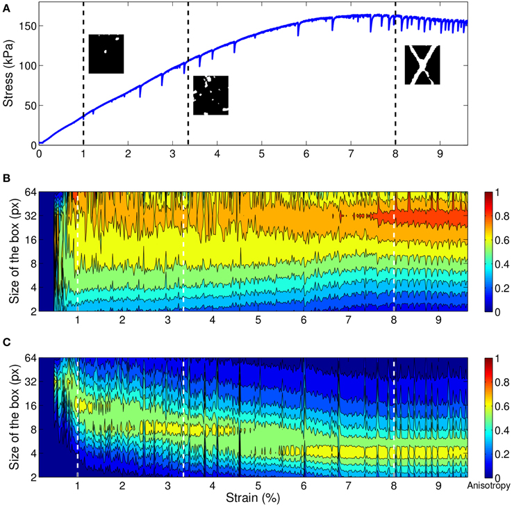
Figure 7. Analysis of correlation patterns in precursors to the rupture of a granular material (Figures 1C–H). (A) Loading curve: deviatoric stress σ_zz − σ_xx vs. the global axial deformation ε = ΔL/L. Inserts : images used for the analysis obtained from the correlation maps of Figures 1D,E,G. (B) Anisotropy vs. strain and box size for the whole experiment (see color code on the right side: red = anisotropic, blue = isotropic). For each value of the deformation 20 consecutive images are used in order to increase the statistics for the calculation of the average of the anisotropy at a given scale. (C) Test of significance: same plot after mixing the pixels of each image. In the three panels, the strain increment between successive images is δ ε = 10⁻⁵.

Figure 7B shows in colorscale the evolution of the anisotropy vs. the size of the boxes used for the image analysis, and vs. the deformation of the sample. Large enough ensemble for the average anisotropy at a given scale are obtained by using 20 consecutive images as representative of the same pattern.

In order to reduce pixel noise at small scales which is very high in the original maps of correlation, and to reduce the effect of a gradient of deformation present at the beginning of the loading (Figure 1D), before anisotropy calculation the maps have been pre-treated as follows : median filter of radius 3, substraction of the average gradient in deformation along the vertical direction, binarization.

The resulting analysis (Figure 7B) shows that from a strain of about 1%, the anisotropy is maximal for scales between 8 and 64 pixels. The decrease of the anisotropy at the largest scale can be understood by the fact that bands tend to appear in two symmetric directions so that at large scale the anisotropy decreases. In this particular case, a quadrupolar rather than dipolar analysis would allow a more detailed description of the conjugate bands system at large scale (Section 2.3.1). Below 1% the data are still partly obscured by the overall gradient of deformation over the sample. The scale of maximum anisotropy increase slightly for strains between 1% and 5% and then stabilizes between 32 and 64 at the end of the process. At given scales, above a size of 16, the anisotropy increases with the deformation.

A test of the accuracy of multiscale analysis is the comparison of the result of the same algorithm applied on an image composed of the same pixels values as the original one, but where the positions of the pixels have been randomly mixed so that potential spatial structurations have been destroyed. Such randomization has been applied on all the images used for the analysis of the emergence of anisotropy in the biaxial test and the result is displayed on Figure 7C. A significant anisotropy appears at decreasing scales during the loading. At small deformation, anisotropy appears only at the largest scales, then the maximal value of the anisotropy appear at smaller and smaller scales. Anisotropy coming from pixel noise is expected for a pattern containing random pixels, yet such noise can only appear when it contains at least two non-zero pixels. Indeed, when a box contains only one non-zero pixel, the barycenter of the box is located on that pixel and the anisotropy is null. It explains why for the images containing few information, as the first example where only 1.2% of the pixels are non-zero (top left inset of Figure 7A), anisotropy only appears for large enough boxes of analysis. When the amount of information increases, pixel noise appears at smaller scales, as the probability for two pixels to be in a smaller box increases.

A test performed with $\overline{\overline{Q}}$ instead of $\overline{\overline{P}}$ (not shown) evidences only a weak effect on Figure 7B. Conversely, the analysis of a random image yields a result very different from Figure 7C: a strong anisotropy is visible at small scales due to boxes with a small number of white pixels, with but especially without strain.

4. Discussion

Our formalism can be related with two existing ones: the Leray regularization, and the optimal anisotropic wavelet transform. The inertia tensor can be compared with existing measurements, such as the anisotropic pair correlation function, the Fourier transform, the Hough transform and the diffusion tensor imaging.

4.1. Link with Existing Theoretical Formalisms

4.1.1. Link with Leray regularization

Let us first explain the historical context of Leray's work. The Navier-Stokes equations (NSE) take the form of partial differential equations describing for the fluid velocity. These types of equations are not suitable for non-differentiable fields, so that one needs both new tools and more general descriptions of the fluid equations to deal with singular fields, as already recognized by Onsager [22]. However, the NSE can still be meaningful in the sense of distributions, i.e., after smearing with smooth test functions ϕ(x, t). Leray [23] worked over a suitable formalism to construct weak solutions of a partial differential equation with singularities, like Euler equation, through a sequence of filtered velocity field u obtained by smearing it at scale with special test functions ϕ_ℓ(x, t) = ℓ⁻³ϕ(x/ℓ). The corresponding velocity field are smooth, and obeys smoothed version of the NSE that describe the behavior of u in a larger phase space, including both the physical space and the scale space. Limiting behaviors for viscosity ν → 0 weak solutions of the NSE can then be obtained through limits of u as ℓ → 0. Leray regularization is an example of function ϕ with interesting properties, albeit (or because) intrinsically anisotropic.

In the spirit of Leray, we introduce a scale transform, with the important difference that we specifically want to extract unbiased anisotropy information. We introduce a spatial coarse-graining (which can be extended to spatio-temporal coarse graining) such that:

$\begin{array}{cc}\overline{u}(b,\ell ,t)={\displaystyle \int \frac{d^{3}x}{{\ell }^3}}u(x,t)F\left(\overrightarrow{k}·\left(\overrightarrow{b}-\overrightarrow{x}\right)\right),& \left(8\right)\end{array}$

where $\overrightarrow{b}$, $\overrightarrow{x}$ and $\overrightarrow{k}$ are vectors (|$\overrightarrow{k}$| = 1/ℓ), and F is any C_∞ non-negative function decaying to zero sufficiently rapidly at infinity (more quickly than x⁻²) and such that ∫ F(x)dx = 1 [24–26]. An example is the Gaussian F(x) = exp(−x²/σ)/(2πσ).

To achieve the link with the inertia tensor, consider the scalar quantity I and take its transform according to Equation (8). By definition, it has the interesting property:

$\begin{array}{cc}\begin{array}{l}{\partial }_{k_j}\overline{I}(b,\ell ,t)={\displaystyle \int \frac{d^{3}x}{{\ell }^3}}(b_j-x_j)I(x,t)F^{\prime }(\overrightarrow{k}·(\overrightarrow{b}-\overrightarrow{x})),\\ {\partial }_{k_j}{\partial }_{k_l}\overline{I}(b,\ell ,t)={\displaystyle \int \frac{d^{3}x}{{\ell }^3}}(b_j-x_j)(b_l-x_l)I(x,t)\\ \times F^{″}(\overrightarrow{k}·(\overrightarrow{b}-\overrightarrow{x})),\end{array}& \left(9\right)\end{array}$

so that ∂_kj∂_kl I(b, ℓ, t) is nothing but $\overline{\overline{P}}$, the inertia tensor of I. Hence Equation (4) appears as a particular case of Leray transform.

This suggests how to generalize Equation (4). If the signal I is a vector rather than scalar quantity, the inertia tensor can be replaced by the scale tensor:

$\begin{array}{cc}\begin{array}{l}{S}_{ij}(\overline{u})={\partial }_{k_j}{\overline{u}}_i(b,\ell ,t)={\displaystyle \int \frac{d^{3}x}{{\ell }^3}}(b_j-x_j)u_i(x,t)\\ \times F^{\prime }\left(\overrightarrow{k}·\left(\overrightarrow{b}-\overrightarrow{x}\right)\right).\end{array}& \left(10\right)\end{array}$

The trace and the antisymmetric part of S yield the divergence and the rotational in scale space, respectively.

4.1.2. Link with optimal anisotropic wavelet transform

The inertia tensor can be compared with the Optimal Anisotropic Wavelet Transform (OAWT) introduced by Ouillon et al. [27] and used in characterization of fracture patterns or heterogeneous porous media [28]. The basic ingredient of OAWT is an anisotropic wavelet, depending on 3 parameters: the scale a, the orientation θ and the anisotropy factor σ. The final output is a rose diagram, representing the typical orientation of a given portion of the image as a function of scale. Its obtention requires the computation at each scale of all the wavelet coefficients as a function of σ and θ. An appropriate decimation of these wavelets coefficients through appropriate thresholding enables, for each scale a, to keep only “optimized” coefficients with given orientation θ_opt and anisotropy σ_opt. The rose diagram is then obtained as a histogram of the optimized orientations or each scale. This method therefore provides the typical orientation as a function of scale at the expense of a waste of computations: most of the computed coefficients are not used.

By comparison, the inertia tensor converges to an isotropic wavelet transform when the wavevector is isotropic. The final output of our method are ellipses, which axes are along the direction of anisotropy and which orientation provides the typical orientation at each scale and each point of the image. The computation of these ellipses requires the obtention of the inertia tensors, that are nothing but the second scale derivatives (derivation with respect to the wavector) of the Leray-like transform (Section 4.1.1) and are very simple to implement numerically. The inertia tensor therefore provides a more direct and conceptually simple way to obtain the same information as the OAWT.

4.2. Comparison with Some Existing Methods

4.2.1. Anisotropic pair correlation function

The pair correlation function of an image is:

$\begin{array}{cc}g\left(\overrightarrow{r}\right)=\frac{\langle I\left(\overrightarrow{x}\right)I\left(\overrightarrow{x}+\overrightarrow{r}\right)\rangle }{\langle I{\left(\overrightarrow{x}\right)}^2\rangle }& \left(11\right)\end{array}$

The average is here taken over all pixels $\overrightarrow{x}$ in a box. The pair correlation function characterizes the dependence in scale r = |$\overrightarrow{r}$| and in direction θ of vector $\overrightarrow{r}$.

Classical uses of g ($\overrightarrow{r}$) average over the direction θ of vector $\overrightarrow{r}$ and only the dependence in scale, g(r), is plotted. A standard use of this function g($\overrightarrow{r}$) is to perform the average over all positions $\overrightarrow{x}$: the box is equal to the whole image. A problem in that case is that $\overrightarrow{x}$ +$\overrightarrow{r}$ does not necessarily belong to the image, and thus image boundary effects have to be taken into account.

Figure 8 plots the pair correlation function for granite images in conditions similar to Figure 5C. Since here we are interested in anisotropy, we can alternatively plot g(θ) for a fixed r, which yields an analysis in direction (Figures 8A,B). Superimposing plots at different values of r yields an analysis in scale and direction (Figure 8C).

FIGURE 8

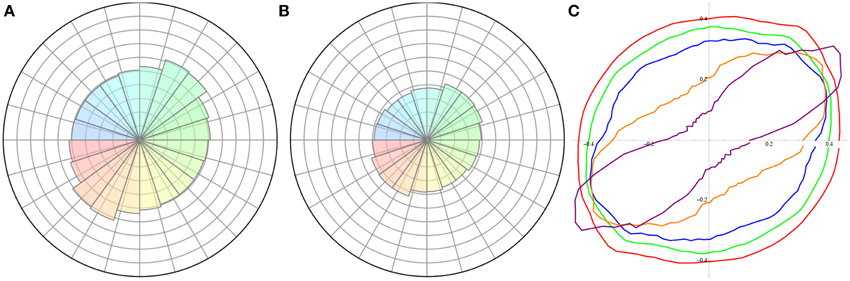
Figure 8. Pair correlation function of the post-rupture granite image (Figure 1B). (A) Polar representation of the pair correlation function. Analysis radius is 8 pixels ; polar angle takes 20 uniformly distributed values between 0 and 2 π. (B) Same with 64 pixel radius. (C) Series of polar plot showing multiple analysis radii: 32 (red), 64 (green), 128 (blue), 256 (orange), and 512 (purple) pixels ; polar angle takes 96 uniformly distributed values between 0 and 2 π.

The pair correlation function detects well the large scale anisotropy. However, if the pattern contains small scale anisotropic structures in various directions, the pair correlation function does not detect an anisotropy at small scale (Figure 8C). This drawback is reminiscent of the anisotropy of our average tensor (Figure 4B).

By splitting the image into smaller boxes (like for the inertia tensor), the pair correlation function too can be measured vs. position, and thus in principle detect small scale anisotropy. However, in practice, the drawback of the pair correlation function is its edge effect, which becomes stronger and stronger when boxes get smaller. We have performed several tests and improvements of pair correlation function on both the granite and granular patterns without being able to significantly measure any small scale anisotropy (data not shown).

4.2.2. Fourier transform

Fourier transform decomposes an image into a set of spatial frequencies which reflect the existence, the spacing and direction of geometric patterns. In each box of a grid, after appropriate windowing (multiplication by a square cosine) that minimizes the edge effects, the local Fourier transform can be calculated. Its norm is maximum in the center of the Fourier space and its decrease is anisotropic. It is possible to quantify the anisotropy of this Fourier transform, for instance by binarizing it and measuring the anisotropy of the resulting cloud of points, yielding the initial pattern's local main direction [29].

Since only the norm (and not the phase) of the Fourier is used, the analysis is insensitive to possible translations of the pattern. This is convenient when different images are averaged, for instance in ensemble average over different experiments. Fourier transform is useful at a fixed scale. However, it suffers the same edge effects as the pair correlation function (Section 4.2.1), so that for a true analysis in terms of both position and scale, the optimal anisotropic wavelet transform (Section 4.1.2) or the inertia tensor are more suitable.

4.2.3. Hough transform

The Hough transform is a tool allowing to detect lines in pictures [30]. We use it on the granular image patterns (Figures 1C–H) to find the preferential direction of the intermittent and permanent shear bands.

The method is based on a characterization of lines in the plane by two polar parameters (ρ, θ), ρ being the distance between the considered line and the origin, and θ the polar angle between the normal to the line and the abscissa. Using this parametrization the whole set of possible lines going through a given point (x₀, y₀) can be written:

$\begin{array}{cc}\rho =x_0\cos \theta +y_0\sin \theta ,& \left(12\right)\end{array}$

so that the ensemble of concurrent lines associated to a single point in the plane is represented by a sinusoid in the (ρ, θ) parameter space, the so-called Hough space. For an image containing N points, the representation in the Hough space will contain N sinusoids (Figures 9A,B). The intersections of those sinusoids give values of the parameters corresponding to lines going through several points of the pattern. For example, the Hough transform of Figure 9A displays several values of the parameters (ρ, θ) for which numerous sinusoids intersects. Lines corresponding to those values of the parameters are drawn in blue on Figures 9A,B, using barycenters of the maximal areas in the plane of parameters (ρ, θ).

FIGURE 9

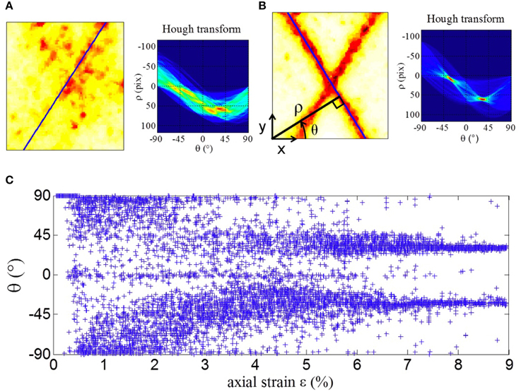
Figure 9. Hough transform of granular material images (Figures 1C–H). (A) Beginning of the loading process (cf Section 3.3). Left : Correlation map. Right: Hough transforms of the correlation map. The contribution of each sinusoid is weighted depending on the value of the correlation of the point of the map, g_I (the weight is 1/g_I if 0.1 < g_I < 0.8, 10 if 0.1 > g_I, 0 if g_I > 0.8). (B) Same as (A), at the end of the loading process. Definitions of notations x, y, ρ, θ. (C) Inclination of the two lines obtained using the barycenter of the two first local maximal areas in the Hough space during the loading process.

As Figure 9A, left displays numerous scattered spots, several intersections are seen in the Hough space (Figure 9A, right) and the areas corresponding to intersections of sinusoids are wide. On the other hand, in Figure 9B, left, where two very clear inclinations are seen on the image, the Hough transform (Figure 9B, right) displays two clear intersections of most sinusoids, indeed corresponding to the principal inclinations in the image.

Figure 9C shows the successive inclinations of the major lines obtained using the Hough transform. For each value of the axial strain, the values of the parameters of the barycenters of the local maximal areas in the Hough space are used. At the beginning of the loading process, the inclinations obtained are scattered but follow a general trend: a monotonous evolution from two symmetric positions starting from almost horizontal to lines inclined at ± 30°.

Since Hough transform and inertia tensor provide different types of outputs, they are complementary rather than directly comparable. Hough transform is highly accurate to analyse the position and direction of well-formed linear structures, such as fibers. The inertia tensor is multiscale; it probes various types of anisotropic structures, not only lines; and it is simpler.

4.2.4. Tensor imaging

In nuclear magnetic resonance images (MRI), normally performed in 3D, it is possible to determine in each voxel the local diffusion coefficient of water molecules. Diffusion can be anisotropic: water diffuses more quickly along one direction than along another; a diffusion tensor, rather than a scalar coefficient, can be determined voxel by voxel. Such diffusion tensor imaging (DTI) can be analyzed to determine privileged directions (oriented distribution function, or ODF), using specific representations like q-ball imaging (QBI). This is instrumental to evaluate the presence and position of fibers, for instance in brain or muscle, using a set of techniques collectively called “tractography” [4, 31].

Both DTI and inertia tensor measure a local anisotropy, which can help to identify fibers by investigate how aligned are the anisotropy directions of neighboring voxels. Both use tensorial formalisms, which make them mathematically robust, adaptable to both 2D and 3D, and amenable to similar representations; both are suitable for averages over different images (for which Fourier transform is sometimes better, see Section 4.2.2). Beside that, DTI and inertia tensor differ strongly; since they use different types of inputs, they are complementary rather than directly comparable.

DTI is a subpixel resolution technique, in the sense that it helps finding fibers even where the actual image obtained by MRI is uniform or at least isotropic. Rather than the anisotroy of the pattern itself, it investigates the anisotropy of a physical property defined at each voxel, which is itself a tensor (the diffusion tensor). Since the scale of study is determined by the timing, amplitude and shape of the gradient pulses, DTI can be made multiscale by performing a new experiment for each scale, even at scales smaller than the voxel size [32].

In other fields, other tensors can be imaged. In mechanics, a local stress or strain tensor can de defined at the scale of resolution of the analysis, or after coarse graining at the scale of a box up to the system size scale [33].

The inertia tensor, much simpler than tensor imaging, is based on a scalar value at each voxel, and determines the anisotropy of the spatial distribution of this scalar among voxels. The anisotropy is a property of the pattern, irrespective of the physical quantity encoded in the scalar value. It is directly multiscale, at scales larger than the voxel size. It detects fibers at scales larger than the voxel size (which Hough transform performs more accurately, see Section 4.2.3). It also probes other types of anisotropic structures.

Equation (4) is tensorial, and thus equally valid in three dimensions, where the analogous of Equation (5) is:

$\begin{array}{cc}\overline{\overline{P}}(\overrightarrow{r},\ell )={\displaystyle \sum _{\text{box}}\left(\begin{array}{ccc}{X}^2& XY& XZ\\ XY& Y^2& YZ\\ XZ& YZ& Z^2\end{array}\right)}I.& \left(13\right)\end{array}$

The set of measurements based on a 3D tensor can be inspired from mechanics: normal differences, ratios of eigenvalues, 2d invariant. Numbers ranging from 0 to 1 to quantify the anisotropy can be inspired from MRI: standard deviation of the three eigenvalues (λ₁, λ₂, λ₃) normalized by their average 〈 λ_i 〉 (“relative anisotropy”) or by their root mean square 〈 λ²_i 〉^1/2 (“fractional anisotropy”); or 1 minus the “volume ratio” (defined as the product of the eigenvalues divided by their average cubed), 1 − λ₁ λ₂ λ₃/〈 λ_i 〉³.

Representations can also be inspired from mechanics or MRI: ellipsoids, bars, color maps.

5. Conclusion

In summary, the proposed method for anisotropy analysis consists in dividing the image into analysis boxes at a chosen scale; in each box an ellipse (the inertia tensor) is fitted to the signal and thus determines the direction in which the signal is more present. This tensor can be averaged in position and/or be used to study the dependence with scale. While this choice is motivated more by the search for simplicity than by any mathematical reason, it is linked with the formalisms of Leray transforms and anisotropic wavelet analysis.

Such protocol is intuitively interpreted, and consistent with what the eye detects: relevant scales, local variations in space, privileged directions. It is fast and parallelizable. It constitutes a versatile toolbox with several variants adaptable to the users' data and needs. It is useful to statistically characterize anisotropies of 2D or 3D patterns in which individual objects are not easily distinguished, with only minimal pre-processing of the raw image, and more generally applies to data in higher dimensions. It is less sensitive to edge effects, and thus better adapted for a multiscale analysis down to small scale boxes, than comparable methods such as pair correlation function or Fourier transform. Easy to understand and implement, it complements more sophisticated methods such as Hough transform or diffusion tensor imaging.

We successfully use it on various fracture patterns (which differ by seven orders of magnitude in spatial scales: the sea ice cover, thin sections of granite, and granular materials), to pinpoint the maximal anisotropy scales. The results are robust to noise and to users' choices. It is possible to distinguish the case where all regions are isotropic, from the case where all regions have anisotropies but in different directions (“powder effect”). Beside the field of fracture, this toolbox could turn useful for granular materials, hard condensed matter, geophysics, thin films, statistical mechanics, characterization of networks, fluctuating amorphous systems, inhomogeneous and disordered systems, or medical imaging, among others.

Author Contributions

Roland Lehoucq, Jérôme Weiss, Bérengère Dubrulle, David Amitrano, François Graner have contributed to design the research; Jérôme Weiss, David Amitrano, Axelle Amon, Antoine Le Bouil, Jérôme Crassous have contributed to acquire the data; Roland Lehoucq, Jérôme Weiss, Axelle Amon, Antoine Le Bouil, Jérôme Crassous, David Amitrano, François Graner have contributed to analyse the data; Roland Lehoucq, Jérôme Weiss, Bérengère Dubrulle, Axelle Amon, Jérôme Crassous, David Amitrano, François Graner have contributed to interpret the results; Roland Lehoucq, Jérôme Weiss, Bérengère Dubrulle, Axelle Amon, François Graner have contributed to draft the manuscript; all authors have contributed to revise the manuscript and have given final approval.

Funding

François Graner belongs to the CNRS consortiums “Foams and Emulsions,” which provided travel funding, and “CellTiss.”

Conflict of Interest Statement

The authors declare that the research was conducted in the absence of any commercial or financial relationships that could be construed as a potential conflict of interest.

Acknowledgments

Antoine Le Bouil, Axelle Amon, and Jérôme Crassous thank Guillaume Raffy for discussions about Hough transform. We thank Cyprien Gay and Davide Faranda for critical reading of the manuscript.

Supplementary Material

The Supplementary Material for this article can be found online at: http://www.frontiersin.org/journal/10.3389/fphy.2014.00084/abstract

Footnotes

1. ^http://rsbweb.nih.gov/ij/

References

1. Mecke K, Stoyan D. (eds). Morphology of Condensed Matter - Physics and Geometry of Spatially Complex Systems, Lecture Notes in Physics 600. Heidelberg: Springer (2002).

Google Scholar

2. Graner F, Dollet B, Raufaste C, Marmottant P. Discrete rearranging disordered patterns, part I: Robust statistical tools in two or three dimensions. Eur Phys J E (2008) 25, 349. doi: 10.1140/epje/i2007-10298-8

Pubmed Abstract | Pubmed Full Text | CrossRef Full Text | Google Scholar

3. Jiao Y, Stillinger FH, Torquato S. A superior descriptor of random textures and its predictive capacity. Proc Natl Acad Sci USA. (2009) 106, 17634. doi: 10.1073/pnas.0905919106

Pubmed Abstract | Pubmed Full Text | CrossRef Full Text | Google Scholar

4. Le Bihan D, Mangin JF, Poupon C, Clark CA, Pappata S, Molko N, et al. Diffusion tensor imaging: concepts and applications. J Magn Reson Imaging. (2001) 13, 534. doi: 10.1002/jmri.1076

Pubmed Abstract | Pubmed Full Text | CrossRef Full Text | Google Scholar

5. Vevatne JN, Rimstad E, Hope SM, Korsnes R, Hansen A. Fracture networks in sea ice. Front Phys. (2014) 2:21. doi: 10.3389/fphy.2014.00021

Pubmed Abstract | Pubmed Full Text | CrossRef Full Text | Google Scholar

6. Fichefet T, Morales Maqueda MA. On modelling the sea-ice-ocean system. Modél. Coupl. Climatol. (1995) 76, 343–420.

7. Weiss J, Marsan D. Scale properties of sea ice deformation and fracturing. CR Phys. (2004) 5, 683–685. doi: 10.1016/j.crhy.2004.08.003

CrossRef Full Text | Google Scholar

8. Marcq S, Weiss J. Influence of sea ice lead-width distribution on turbulent heat transfer between the ocean and the atmosphere. Cryosphere (2012) 6, 143–156. doi: 10.5194/tc-6-143-2012

CrossRef Full Text | Google Scholar

9. Weiss J. Scaling of fracture and faulting in ice on Earth. Surv Geophys. (2003) 24, 185–227. doi: 10.1023/A:1023293117309

CrossRef Full Text | Google Scholar

10. Dyer H, Amitrano D, Boullier AM. Scaling properties of fault rocks. J Struct Geol. (2012) 45, 125–136. doi: 10.1016/j.jsg.2012.06.016

CrossRef Full Text | Google Scholar

11. Heilbronner R, Keulen N. Grain size and grain shape analysis of fault rocks. Tectonophysics (2006) 427, 199–216. doi: 10.1016/j.tecto.2006.05.020

CrossRef Full Text | Google Scholar

12. Sammis CG, King G, Biegel R. The kinematics of gouge deformation. PAGEOPH (1987) 125, 777. doi: 10.1007/BF00878033

CrossRef Full Text | Google Scholar

13. Sammis CG, Biegel R. Fractals, fault gouge, and friction, PAGEOPH (1989) 131, 255–271. doi: 10.1007/BF00874490

CrossRef Full Text | Google Scholar

14. Sammis CG, King GCP. Mechanical origin of power law scaling in fault zone rock. Geophys Res Lett. (2007) 34, L04312. doi: 10.1029/2006GL028548

CrossRef Full Text | Google Scholar

15. Amitrano D. Brittle-ductile transition and associated seismicity: Experimental and numerical studies and relationship with the b-value. J Geophys Res. (2003) 108 B1, 2044. doi: 10.1029/2001JB000680

CrossRef Full Text | Google Scholar

16. Nedderman RM. Statics and Kinematics of Granular Materials. New York, NY: Cambridge University Press (1992).

Google Scholar

17. Eshelby JD. The Determination of the Elastic Field of an Ellipsoidal Inclusion, and related problems. Proc R Soc Lond A (1957) 241, 376–396. doi: 10.1098/rspa.1957.0133

CrossRef Full Text

18. Le Bouil A, Amon A, Sangleboeuf JC, Orain H, Bésuelle P, Viggiani G, et al. A biaxial apparatus for the study of heterogeneous and intermittent strains in granular materials. Granul Matter (2014) 16, 1–8. doi: 10.1007/s10035-013-0477-x

CrossRef Full Text

19. Crassous J. Diffusive wave spectroscopy of a random close packing of spheres. Eur Phys J E (2007) 23, 145. doi: 10.1140/epje/i2006-10079-y

Pubmed Abstract | Pubmed Full Text | CrossRef Full Text | Google Scholar

20. Erpelding M, Amon A, Crassous J. Diffusive wave spectroscopy applied to the spatially resolved deformation of a solid. Phys Rev E (2008) 78:046104. doi: 10.1103/PhysRevE.78.046104

Pubmed Abstract | Pubmed Full Text | CrossRef Full Text | Google Scholar

21. Amon A, Nguyen VB, Bruand A, Crassous J, Clément E. Hot spots in an athermal system. Phys Rev Lett. (2012) 108:135502. doi: 10.1103/PhysRevLett.108.135502

Pubmed Abstract | Pubmed Full Text | CrossRef Full Text | Google Scholar

22. Onsager L. Statistical hydrodynamics. Nuovo Cim. (1949) 6(Suppl.), 279–287, see also 249, 261.

Google Scholar

23. Leray J. Essai sur le mouvement d'un liquide visqueux emplissant l'espace. Acta Math. (1934) 63, 193248. doi: 10.1007/BF02547354

CrossRef Full Text

24. Eyink GL. The Renormalization Group method in statistical hydrodynamics. Phys Fluids A (1994) 6, 3063–3078. doi: 10.1063/1.868131.

Pubmed Abstract | Pubmed Full Text | CrossRef Full Text | Google Scholar

25. Eyink GL, Sreenivasan KR. Onsager and the theory of hydrodynamic turbulence. Rev Mod Phys.(2006) 78, 87135. doi: 10.1103/RevModPhys.78.87

Pubmed Abstract | Pubmed Full Text | CrossRef Full Text | Google Scholar

26. Eyink GL. Dissipative anomalies in singular Euler flows. Physica D (2008) 237, 1956–1968. doi: 10.1016/j.physd.2008.02.005.

CrossRef Full Text | Google Scholar

27. Ouillon G, Sornette D, Castaing C. Organisation of joints and faults from 1-cm to 100-km scales revealed by optimized anisotropic wavelet coefficient method and multifractal analysis. Nonlin Proc Geophys. (1995) 2, 158. doi: 10.5194/npg-2-158-1995

CrossRef Full Text | Google Scholar

28. Qi X, Neupauer RM. Wavelet analysis of characteristic length scales and orientation of two-dimensional heterogeneous porous media. Adv Water Resour (2010) 33, 514. doi: 10.1016/j.advwatres.2010.02.003

CrossRef Full Text | Google Scholar

29. Bosveld F, Bonnet I, Guirao B, Tlili S, Wang Z, Petitalot A, et al. Mechanical control of morphogenesis by Fat/Dachsous/Four-Jointed planar cell polarity pathway. Science (2012) 336, 724. doi: 10.1126/science.1221071

Pubmed Abstract | Pubmed Full Text | CrossRef Full Text

30. Duda RO, Hart PE. Use of the Hough transformation to detect lines and curves in pictures. Comm ACM (1972) 15, 11–15. doi: 10.1145/361237.361242

CrossRef Full Text | Google Scholar

31. Descoteaux M. High Angular Resolution Diffusion MRI: From Local Estimation to Segmentation and Tractography. Human-computer interaction, Ph.D. thesis (in english), Université Nice Sophia Antipolis (2008). Available online at: https://tel.archives-ouvertes.fr/tel-00457458

32. Ingo C, Magin RL, Colon-Perez L, Triplett W, Mareci TH. On random walks and entropy in diffusion-weighted magnetic resonance imaging studies of neural tissue. Magn Reson Med. (2014) 71, 617–627. doi: 10.1002/mrm.24706

Pubmed Abstract | Pubmed Full Text | CrossRef Full Text | Google Scholar

33. Marsan D, Stern H, Lindsay R, Weiss J. Scale dependence and localization of the deformation of Arctic sea ice. Phys Rev Lett. (2004) 93:178501. doi: 10.1103/PhysRevLett.93.178501

Pubmed Abstract | Pubmed Full Text | CrossRef Full Text | Google Scholar