Efficient computation and statistical assessment of transfer entropy

1. Introduction

Natural science strives to find correlations in empirical data to identify patterns that might indicate the presence of causation. Frequently, such data consists of time series of a random variable X with a recorded data set of {x_t}. The stochastic process giving rise to {x_t} might have memory, so that x_t is correlated with x_{t + τ} over a history of length τ.

Furthermore, X and another observable Y might be correlated; if such two time series are correlated or have some form of interdependence, a more sophisticated way to quantify the connection—beyond, for example, the simple Pearson linear correlation coefficient—is the transfer entropy (TE) proposed by Schreiber [2].

The TE is asymmetric, so that TE(X → Y) ≠ TE(Y → X). This difference indicates a direction of information flow and thus potential causation from one variable to the other. This distinguishes the TE from the time-delayed mutual information (TDMI) which has no sense of “direction” [3].

Besides the conceptual advantages of the TE, current approaches of using TE [4, 5] face two major problems which we address in this work: (a) computation of the TE can be done directly using simple arrays for the data, but only inefficiently so, and, (b) while we can use the asymmetry TE(X → Y) ≠ TE(Y → X) to guess on the direction of information flow, the TE itself does not allow for a statistical assessment of the significance of such flows and their respective directions.

To address the second issue we contribute with this study:

• We develop a statistical testing procedure that relies on the so called Z-test. We show that, indeed, the Z-scores give sensible answers in control- and tunable experiments while a naive TE-application gives inconsistent answers.

• For the Z-tests we propose two different null models of independence between X and Y (the first one for complete independence between all measurements and the second one to maintain intrinsic correlations of a potential “driving” system X while assessing the dependence of Y on the intrinsic dynamics of X).

• We argue about parallelizability and efficient implementation of this Z-test based method. We show that our implementation's parallelism is close to optimal.

• We offer the full implementation of our C++-library for download under the GPL2 license¹.

These contributions are illustrated in the experimental part of this study in Sections 5 and 6 by applying the theory of Section 3 and code to two examples of interdependent times series in Section 4. Before, we briefly review the TE and general information theory and in the next section.

2. Information Theory and Transfer Entropy

The Shannon entropy measures the (dis)order in a data set or a model [6]. If p(x) is the probability of a symbol x for a random variable X with a domain of definition _X, then the Shannon entropy reads:

where we use the fact lim_{ϵ → 0} ϵ · log ϵ = 0. From hereon, we will use log₂ and log interchangeably.

Now, in “traditional information theory” the Kullback-Leibler divergence (DKL) is one measure of the interdependence of two random variables X and Y [7] whose probability distributions are p_X and p_Y and whose outcomes are from a set : = _X ∩ _Y.

which is well defined as long as _X ⊆ _Y. This DKL-based approach has, however, two short-comings: neither does it include a “direction” of the information flow, nor does it include a chronological ordering. Especially, any reference to chronological order would be most desirable to identify potential causation as “The cause must be prior to the effect” [8].

Due to this, [2] developed the concept of transfer entropy: first, to include time order into the analysis we can use the entropy rate H_r of the process {x_t}. For convenience, we will assume that the time is given on a regular grid of equidistant time intervals τ and use counters like n to enumerate the time points, thus n: = ⌊t/τ⌋. Were appropriated we will use n and t interchangeably.

$\begin{array}{cc}{H}_r=-{\displaystyle \sum _{x_{n+1},x_n^m}p}(x_{n+1},x_n^m)\log \left(p(x_{n+1}|x_n^m)\right)& \left(3\right)\end{array}$

Here, x^m_n is an m-tuple of measurements at time steps n, n − 1, …, n − m + 1. We employ the same history length m for both data sets {x_n} and {y_n}, while the general formulation by Schreiber [2] allows different m and m′ for {x_n} and {y_n}, respectively.

Note, that building histograms p(x_{n + 1}, x^m_n) and p(x_{n + 1} | x^m_n) is – even for intermediate value of m—already difficult due to the “curse of dimensionality” [9]. This effect is caused by the exponentially increasing number of buckets in the histogram with increasing dimension (m). The unwanted effects of sparsely populated histograms due to small data sizes and the curse of dimensionality is (partially) resolved by our one-sided testing procedure introduced in Section 3 as we derive statistical significance levels.

Following Schreiber [2], the transfer entropy is then an analogous extension of the entropy to the DKL as in Equation (2) to include the effect of another time series {y_n}.

$\begin{array}{cc}\text{TE}\left(Y\to X\right)={\displaystyle \sum }p(x_{n+1},x_n^m,y_n^m)\text{log}\frac{p(x_{n+1}\mid x_n^m,y_n^m)}{p(x_{n+1}\mid x_n^m)}& \left(4\right)\end{array}$

Figure 1 illustrates the concept of using combinations along the temporal order of the data sets {x_n} and {y_n} to compute the TE.

FIGURE 1

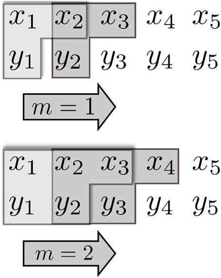
Figure 1. Schematic representation of a TE calculation for a time window of m = 1 (top) and m = 2 (bottom); herein m is the size of the time window which “slides” along the sequentially ordered data {x_t} and {y_t}. The “L”-shaped collections of singular data give rise to the tuples of data x_{n + 1}, (x_n^m, y_n^m), and (x_{n + 1}, x_n^m, y_n^m) used in building the p(x_{n + 1} | x_n^m, y_n^m).

Equation (4) is a generalization of the concept of Granger causality [10] for a particular choice of statistical model for the X and Y—namely Gaussian processes. Eventually, TE and Granger causality are equivalent for Gaussian variables [11]. This equivalence inspired us to assign statistical significance based on Z-scores which explicitly correspond to percentiles in the case of Gaussian variables.

3. Statistical Significance Testing and Z-Scores

From Equation (4) we can immediately deduce [1] that the TE is a difference of entropies, thus a relative entropy:

$\begin{array}{cc}\text{TE}\left(Y\to X\right)=H\left(x_{n+1}\mid x_n^m\right)-H\left(x_{n+1}\mid x_n^m,y_n^m\right)& \left(5\right)\end{array}$

Here, H(… | …) is the conditional entropy where we measure the entropy in the first argument conditioned on the second. More precisely,

where p(x_{n + 1} | x^m_n) is the conditional probability of x_{n + 1} given the m-time window history x^m_n. A similar formula can be derived for H(x_{n + 1} | x^m_n, y^m_n) by replacing p(x_{n + 1} | x^m_n) with p(x_{n + 1} | x^m_n, y^m_n).

Note that entropies are always non-negative. Obviously, an upper bound for the TE is therefore H(x_{n + 1} | x^m_n) and one upper bound for this is log |_X|. Therefore, the scale of the TE is determined by the size of the “event set” _X. In general, it is difficult, if not impossible, to quantitatively compare TE values for a variable X and another one $\tilde{X}$ which have differently sized “event sets” _X and _$\tilde{X}$.

A method to account for different scales and allow an interpretation along the lines of statistical significance testing is the computation of a Z-score.

For a given data set (X, Y) the TE is a random variable as it depends on the random variables x₁, …, x_N, y₁, …, y_N with N the length of the time series. For such a random variable TE we can compute the so-called Z-score as follows:

$\begin{array}{cc}Z(\text{TE})=\frac{\text{TE}-{\overline{\text{TE}}}_s}{\sigma ({\text{TE}}_s)}& \left(7\right)\end{array}$

where TE_s is the (arithmetic) mean of a (computational) sample s of values under a null hypothesis of independence and σ(TE_s) is the respective standard deviation of the sample.

Thus, we can interpret Z(TE) as the deviation of the empirical value TE from the mean of the null model expressed in units of standard deviation. Assuming a normal distribution of the TE values, Z-scores correspond directly to one-tailed p-values. It is important for the subsequent parts of this paper, to keep in mind that negative Z-scores and those close to zero allow for an important interpretation. Z < 0 or Z ≈ 0 implies that the TE of the original data cannot be distinguished from pure random samples or shows in almost all cases less information between X and Y than a randomized sample.

In our quest to extract signatures of causal relations, those cases with significantly large Z are relevant. Note, that our Z computations allow for the statistical assessment while a few previous studies focused on the influence of “background noise” and its compensation by computational means [12, 13].

Naturally, the null hypothesis in causality detection is independence. Then, a “computational null model” in entropy normalizations shuffles the order of elements in one data set [14]. The chronological order is destroyed and thus the m-tuple based histograms p(x_{n + 1}, x^m_n) become “flat.” This method maintains the overall distribution of events and thus the marginal distributions p(x) and therefore the local entropy H(x). The values obtained under this null hypothesis are called Z in the subsequent parts of this paper.

Now, one could argue that in the case that X drives Y the intrinsic correlation among time ordered x_t should not be randomized to retain the internal dynamics of X as we are only interested in potential correlations between the driving system x_t and the observable effects in y_t. We also use this null and shuffle only the order of y_t. Results are then named Z*.

Note, that we will perform both procedures for a computationally created sample of size N_s which is obtained by shuffling the order of the real data randomly, thus destroying potentially existing time-ordering and correlation (either in x_t and y_t [Z] or in y_t alone [Z*]).

4. Examples and Test Systems

We illustrate the concepts of our approach by applying TE to two controllable test systems that were used to generate synthetic data sets. We describe both systems below:

4.1. Coupled Logistic Maps

We follow Hahs and Pethel [15] who proposed an anticipatory system to study transfer entropy. It is based on an unidirectional coupled chaotic logistic map.

$\begin{array}{cc}f(x)=r·x·(1-x)& \left(8\right)\end{array}$

The logistic map parameter r will be set to a fixed value of 4 and thus operating in the chaotic regime. Then, the dynamics of the coupled systems (x_t, y_t) is given by:

$\begin{array}{cc}\begin{array}{l}{x}_{n+1}=f(x_n)\\ y_{n+1}=(1-\xi )·f(y_n)+\xi ·g_{\alpha }(x_n)\end{array}& \left(9\right)\end{array}$

Here, the first time series (x_t, called the driving system) is the logistic map. The response system y_t incorporates two factors: (1) the parameter ξ ∈ [0, 1] represents the coupling strength of the systems x_t and y_t and (2) the coupling function g_α should include an anticipatory element. Hahs and Pethel [15] used

$\begin{array}{cc}{g}_{\alpha }(x)=(1-\alpha )·f(x)+\alpha ·f(f(x))& \left(10\right)\end{array}$

g_α has a parameter α ∈ [0, 1] that modulates the anticipation with respect to the driving system x_t. In the extreme case of ξ = 1 and α = 1, the time series y_t anticipates x_t exactly; for ξ = 0 the systems are decoupled and therefore not correlated at all. Figure 2 illustrates the influence of both parameters on the generated data series.

FIGURE 2

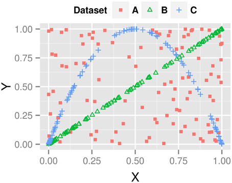
Figure 2. Correlations plots (x_t vs. y_t) for the anticipatory system of Equation 9. A, red squares: independent dynamics (α = 0, ξ = 0); B, green triangles: y_t is driven toward x_t (α = 0, ξ = 1); C, blue crosses: y_t is driven to future state of x_t (α = 1, ξ = 1).

4.2. A Markov Chain Example

While the logistic map of Section 4.1 is deterministic, we add a probabilistic system in the form of a Hidden Markov Model (HMM) that is built from a driving signal² of two states x_t ∈ {A, B} or of four states $\tilde{x}$_t ∈ {A, B, C, D}. The second component is the emitted symbol stream of the HMM y_t, $\tilde{y}$_t ∈ {a, b} with just two states.

Table 1A contains the transition probabilities for the transition from a state x_t to the new state x_{t + 1}. The emitted symbol y_{t + 1} is then drawn – based solely on the state x_{t + 1} – following the probabilities in Table 1B.

TABLE 1

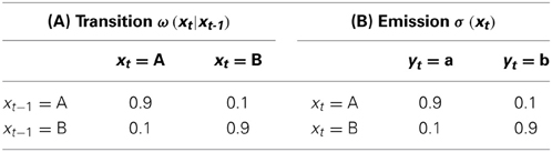
Table 1. Transition ω(x_t | x_{t − 1}) and emission σ(x_t) probabilities of our HMM1.

Our second HMM uses more internal states. The probabilities in Table 2B are chosen in such a way, that the y_t and $\tilde{y}$_t emissions can be compared with respect to the internal states. Note, that the Perron-Frobenius theorem and the fact, that the ω-matrices of Tables 1, 2 are stochastic, leads to the insight that the two states in x_t and the four internal states in $\tilde{x}$_t are equally likely for t → ∞.

TABLE 2

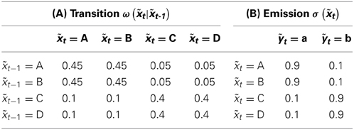
Table 2. Transition ω($\tilde{x}$_t | $\tilde{x}$_{t − 1}) and emission σ($\tilde{x}$_t) probabilities of our HMM2.

With the help of these two models we want to investigate, whether (a) we can use the TE to obtain information on the internal state from the emitted symbols, (b) how the complexity of the internal HMM organization (2 vs. 4 internal states) influences the TE, and (c) illustrate how the Z-score normalization of Section 3 supports identification of such dependencies.

5. Computational Results

5.1. Histogram Building and Internal Parameters

First, we want to get insight into an important aspect of all empirical studies on entropies: how to accurately build histograms, thus frequencies, as estimators for the probabilities in Equation (4). To this end, we follow the rationale of Hahs and Pethel [15] for the anticipatory system of Equation (9). Obviously we want the resolution (meaning the number of bins used for discretization) to be able to capture the causality X → Y while dismissing any signal for Y → X. In Figure 3 we illustrate this for an anticipatory system with α = 1, ξ = 0.4. Clearly, we obtain a valid, distinctive signal from four bins on. Therefore, we will use in the subsequent parts of our computational study four and more bins.

FIGURE 3

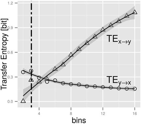
Figure 3. The figure shows the TE as function of the number of bins in the histogram creation (based on a data set of size 10⁶ for the system of Section 4.1), thus the discretization scheme employed (for details see Hahs and Pethel [15]. The lines are fits to local polynomial regressions using the method of Cleveland and Grosse [16]. The gray areas represent the confidence interval (p = 0.95) of the polynomial fit. The intersection point is located at a value of around 4. Below this we obtain a false assignment of information flow (Y → X), while above the order of TEs is correct (TE(X → Y) > TE(Y → X)).

Now, that we have established a lower bound on the number of bins we need to deal with, we turn our attention to the ability of Z and/or Z* scores to improve upon raw TEs. Here, any sensible approach must be able to improve the detection of directionality in the information flow, that is, the coupling of y_n to the dynamics of x_n and its respective history.

5.2. Application to the Coupled Map System

Figure 4 show the results. In the top row we notice that for small data sets (some 2⁸ data points) we cannot distinguish—based solely on the TE alone—between an existing coupling and vanishing one. And even for some 2⁹ data points it is still not possible to correctly judge on the information flow x_n ↔ y_n.

FIGURE 4

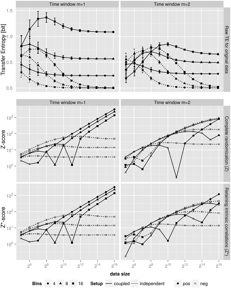
Figure 4. Top: Dependency of TE on the data size, that is the number of samples in the creation of the histograms. The coupled systems (full lines) were created with α = 1, ξ = 0.4 (see Equation 9) and time window of one (left) and two (right). For the independent system (dashed lines) we set both parameters to zero. Clearly, for the latter system the non-existing information flow TE_{x → y} manifests itself only after some 2¹⁴ data points. Values are the mean of 1000 independent replicas of data. Error bars represent the standard deviation. Middle and Bottom: Z-scores for the TE of the top panel for the respective time windows. The middle row uses a shuffling approach that randomizes both vectors X and Y, while the bottom row uses the shuffling model that preserves the intrinsic correlation of the “driving” vector by only shuffling the “driven” vector. Note, the Z-scores for the independent system are negative, we therefore only show the absolute value to be able to use a logarithmic scale. Clearly, the Z-scores for the independent system saturate at a negative, thus insignificant level, while the coupled system (full lines) show significant statistical power that continues to improve with increasing number of data points. The observations depend quantitatively on the number of bins of the histograms; however, the qualitative assessment is the same for number of bins ∈ [4, 8, 16].

Note, that the Z and/or Z*-scores of Equation 7 in the middle and lower rows of Figure 4 are negative for the independent systems and thus imply no information flow. Therefore, only our Z and/or Z*-scores (see Equation 7)—which are computationally much more involved—are able to hint on potential causal relation for small data sets.

It is noteworthy, that even for 2⁴ data points the Z and/or Z*-scores for the independent system are negative and thus the empirical TE for this system is found to be insignificant. Note, that this finding does neither depend on the used number of bins.

For the coupled system (full lines in Figure 4) we find similar results. In particular, we notice an important effect: saturating Z-scores at values of Z ≈ − 10¹ indicate a non-causal relation, while monotonously increasing and thus data size dependent Z-scores for the present coupling show that the more data we deal with, the more significant the finding on the coupling becomes.

It is noteworthy, that computing the Z and/or Z* values at different history window sizes m supports the identification of the internal time scale(s) of X and Y. The (positive) Z and/or Z*-scores grow with a fixed exponent (1/2) as a function of data size for m = 1 and the anticipatory system of Section 4.1 which has an internal time scale of one. Now, when we use m = 2 in our procedure, the scaling of Z and/or Z* is changed qualitatively and does not follow a simple law. We can therefore use our Z and/or Z* approach additionally to estimate the internal time scales.

5.3. Application to the Hidden Markov Models

Now, that the Z and/or Z*-scores contribute insight, we continue our investigation by applying TE and its Z and/or Z*-score assessment to the HMM model of Section 4.2. The results are shown in Figures 5A–C. Figure 5A shows that the overall TE for the causal relation x → y is larger than the one for the more uncertain relation y → x. The findings do not depend on the complexity of the internal driving dynamics as is evident from comparing HMM1 and HMM2 in the figure.

FIGURE 5

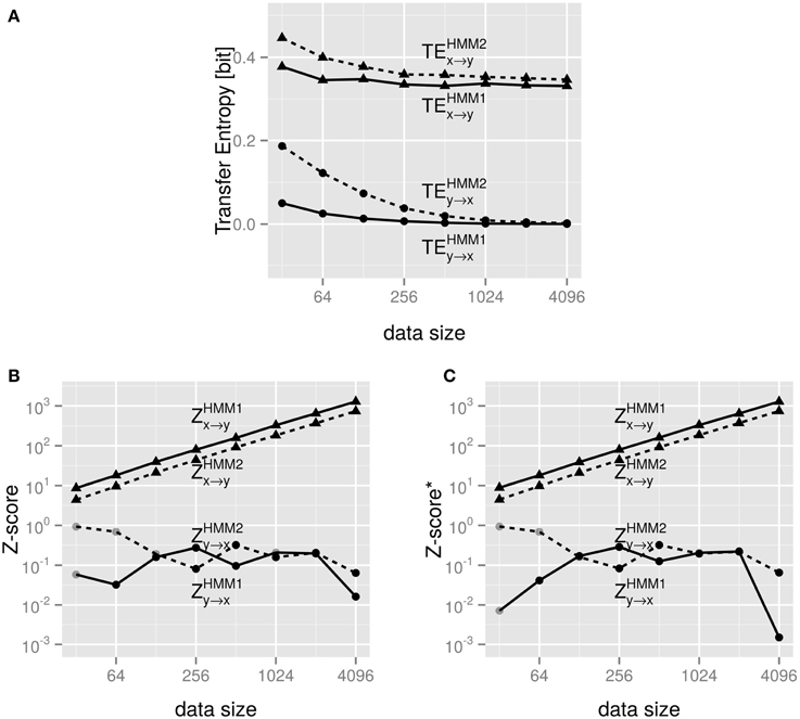
Figure 5. (A) shows the TE for the coupled Hidden-Markov-model of Section 4.2 emitting varying number of data points. (B) shows the Z-scores of the same data used in (A). The data sets were created with the transition probabilities shown in Tables 1, 2, respectively. Gray points indicate negative values, for which we show the absolute value, so that we can still use a logarithmic scale on the y-axis. Full lines are for HMM1 in Table 1 and dashed lines for HMM2 of Table 2. (C) show the same for Z*.

Still, it remains an open question how to compare the TE_{x → y} and TE_{y → x}. They are numerically different, but is this a significant difference? Figure 5B answers this question: the Z scores are orders of magnitude different; clearly, the Z-score computation show significant differences between Z_{x → y} ≈ 10¹ and Z_{y → x} ≈ 10⁻¹ for very small data sets. This difference gets even more pronounced for “reasonable” sized data sets (~ 256 and above).

Again, we find that the Z-score increases monotonously with the data set size. This indicates a positive, synergistic influence of the data quality on the statistical significance – an effect one can expect based on basic statistics.

As expected the (positive) values of Z and Z* do not differ for these systems as they are Markov-Models and thus the null models in Z and Z* are equivalent for the Markov property.

At this point, we have shown that the Z-score normalization contributes significant insight into causal relationships. This was possible due to the test systems that allowed us to manipulate these causal or probabilistic relationships among observables.

However, the tremendous advantages come with a price: increased computational demands. In the next section we discuss how we cope with this drawback and how insight from computer science can help computational physics to improve upon performance issues.

6. Computational Efficiency, Parallelization, and Algorithmics

As one of us recently argued [17], computational physics could greatly benefit from close collaborations with computer scientists, especially in the fields of algorithmics and high-performance computing. Unfortunately, these communities seem to have somewhat diverged despite their fruitful history. Here, we will illustrate the huge gains possible. As the Z and/or Z*-score normalization is an involved procedure, we must first assess how many samples N_s we need to obtain any relevant sampling for the Z and/or Z*-score calculation of Equation (7).

From previous work on entropies [18] we obtain a ballpark-figure for the lower bound on N_s of some 50–100 shufflings. Accordingly, the Z and/or Z*-score procedure is some two orders of magnitude more computationally expensive than the simple TE calculation³.

Does the size of the data set influence our computational resource requirements? In Figure 6 we answer this. Clearly the computational resources needed are proportional to the size of the data set (curves are displaced by a constant factor). The history length m in Equation (4), however, has a non-dramatic influence on the overall computing time. This is due to our first code optimization: we use special histogram data structures that cope with the sparse structure of the histograms for the probabilities p(x_{n + 1} | x_n^m, y_n^m) etc.: whenever there is correlation the histograms are only sparsely populated. Even for the shuffled histograms this assessment holds, although for a different reasons: due to the “curse of dimensionality” only a few data points are randomly distributed in a rather large space, thus the histograms are still sparsely populated. We therefore can store histogram entries in a list of non-vanishing entries, implicitly assigning zero occupancy to any p(…) histogram entry which does not occur in the list. Depending on the system under investigation this reduces the scaling of the memory requirements from (c^m) with a constant c to some more manageable amount. More important, though, is the effect on the computational time: we do not need nested loops of depth m to iterate over all entries. Rather, we just go over the linear list that represents the non-vanishing entries. This list has in the worst-case the same length as the number of buckets in the naive, multi-dimensional histogram. But typically, it is small as can be deduced from Figure 6. In our implementation with used an associative map with vector-like structure representing bucket identifiers as keys and counts as values. Since many parts of the computation filling these associative maps depend heavily on the window size, knowing the window size at compile-time offers many opportunities for optimizations by the compiler.

FIGURE 6

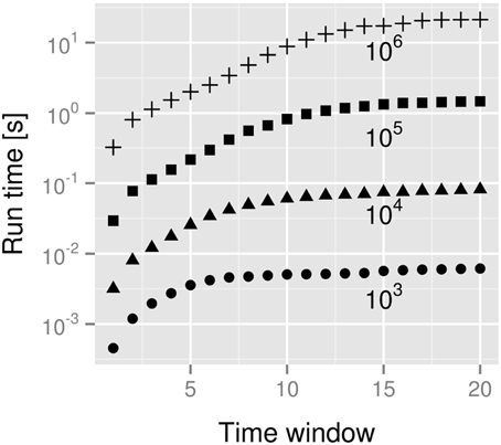
Figure 6. Dependency of the run time of the size of the data set (s). Data sets were created for sizes from 10³ to 10⁶ indicated at the respective curves. Standard deviations were smaller than 0.0015 and error bars therefore omitted.

In fact, the above mentioned bucket identifiers for the histograms are nothing else than integer-coded values x_t and y_t. For accessing associative map entries via keys it is much more efficient to map m-dimensional keys (the integer-encoded x_t, x_{t + 1}, …, x_{t + m}) to one single integer. This scales in a naive implementation, however, with m and involves explicit loops.

In order to obtain pre-compilation and potential loop-unrolling benefits in computing the single-integer-keys we used C++'s template facilities. We decided to let the code use either template instances up to a maximum time window size m_max or decide during run-time whenever m > m_max to iteratively create keys.

For such pre-compiled histograms we found the results of Figure 7. The performance increase can be significant: for a time series generated with 10⁵ data points the wall computation time decreases from about 570 to 370 s on a Core i7 920 Desktop PC. Although with small data sets the effect can be neglected, this shows how pre-compilation will be beneficial for large time series and time windows. The program size increases with the compile-time parameter m_max of explicitly allocated histogram dimensions: ca. 550 kB for m_max = 1 and 5.9 MB for m_max = 100, a noticeable effect, but nevertheless negligible on modern machines.

FIGURE 7

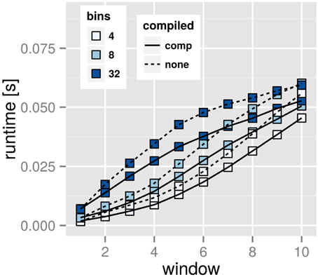
Figure 7. Performance boost through pre-compiled time windows. The dotted lines represent calculations with a compile-time setup of time window m_max = 1. The straight lines represent the same calculation for a compilation setting of time window m_max = 30. Note, that after setting m_max during compile-time we can still vary m during run-time. The timings are means of 1000 independent runs each. Note, that the improvement reaches up to 35% across the board.

The second performance improvement—parallelization—is even more stunning. Our implementation supports multi-threaded calculations of the null model based on the aforementioned shufflings. Since a single shuffle run is independent to others⁴ they can be easily parallelized. To that end we used OpenMP and ran benchmarks that show how efficient the library runs on commodity, multi-core hardware.

Our shuffling procedure(s) are “embarrassingly parallel” [19] as the computations are data parallel and compare to previous approaches [20]. Still, there might exist substantial overhead (e.g., I/O) that renders any parallelization attempt futile. Figure 8 shows—for different hardware architectures—how the speedup⁵ S depends on the number of used CPU cores N. According to Amdahl's law [21] the speedup follows

$\begin{array}{cc}S[N]=\frac{1}{(1-P)+\frac{P}{N}}& \left(11\right)\end{array}$

with the proportion of parallelizable code P. We found P to be 99% for the AMD architecture and 97% for Intel hardware, respectively. This implies, that our parallelization approach has its limitations: for some 100 cores the overhead like IO would correspond to 50% of the overall computation time and thus for architectures like the Intel Phi additional and more involved parallelization approaches are necessary.

FIGURE 8

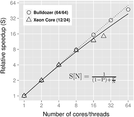
Figure 8. Speed up with respect to number of CPU cores used N. We performed the benchmarks for two different CPU architectures to illustrate the transferability of the used parallelization approach. In parentheses are the number of physical CPU cores and available threads on the very same CPU. The fits are nonlinear least square fits. The fitted parameter P is 0.9945 with a standard error of the mean (SEM) of 10⁻⁴ for the AMD and 0.9732 (SEM = 10⁻³) for the Intel architecture.

7. Conclusions and Outlook

Transfer entropy (TE) is – like the related (time-delayed) mutual information or other schemes of information theory [22] – efficiently computable whenever the sampling space consists of a set of discrete symbols and in low dimensions, that is with a short history window and makes it therefore an interesting analysis approach to correlated data.

While TE is a relative entropy, it was shown [11] that it is closely related to the notion of Granger causality. As such it suffers from a problem related to effect size: the value itself must be assessed for its significance. One way to achieve this is Z-score computation, which directly implies one-sided statistical testing.

Here, we have shown, that Z-score normalization contributes significant new insight, resolves the harming effects of data size problems. We illustrated this by involved computations on two test systems, both of which can be controlled for their “degree of causality.” Furthermore, we propose a more involved null model of independence (named Z*) that is unique for the TE-setting and retains intrinsic correlations in the “driving” time series while assessing the correlation of the “driven” portion to the first one. We found this overall approach to be able to determine internal time scales, but more importantly, to overcome problems with small data sets and assign statistical significance to TE values.

For simple systems which conform to the Markov property we could show that the Z and Z* procedures return consistent answers.

Previously, Waechter et al. [18, 23] implemented Z-score normalization using graphical processing units (GPUs) for simpler entropy concepts than the TE – in particular those without the “curse of dimensionality” [14]. Here, we performed extensive benchmarking and were able to develop a highly optimized code that can be efficiently employed on modern multi-core architectures.

In the future, we plan to apply the methodology and the library to problems in biophysics and systems biology—fields in which research is mainly focused on the search for correlations and potential causal effects in experimental data and where—due to the large number of individual time series that might be correlated, sometimes up to thousands—efficient TE computations are necessary. For N simultaneously recordings of time series we have to compute N · (N − 1) TE measures due to the TE asymmetry. Previously, typical N used were N ≈ 140 in molecular biophysics [24], N = 64 in neuroscience [25], and from N = 32 [26] over N = 100 [27] up to N = 1400 in gene regulation [28].

The overall improvements on real-world running times that we achieved render the present approach applicable to real-world scenarios: Kamberaj and van der Vaart [24], for example, need to analyze all N² combinations of the N = 140 time series. This implies a difference between 135 days (if a single run with some 200 shuffles takes 10 s) in comparison to 22 years (for 10 min for a single computation). Clearly, these improvements are helpful as the latter scenario would most likely be a show-stopper.

Furthermore, in (molecular) biophysics, were memory effects could play a substantial role, the difference between Z and Z* can be used to assign importance to intrinsic correlations within the “driving” system for the causal relationships present.

Author Contributions

All authors developed software and wrote documentation. PB performed numerical computations; KH conceived the study. All authors reviewed the paper and agree on its content.

Conflict of Interest Statement

The authors declare that the research was conducted in the absence of any commercial or financial relationships that could be construed as a potential conflict of interest.

Acknowledgments

KH gratefully acknowledges financial support by the Deutsche Forschungsgemeinschaft under grants HA 5261/3-1 and GRK 1657 (project 3C). This paper uses a software package written by PB, DB, DS, NW, JW, and KH. This implementation is freely available under the GPL 2 license. It can be downloaded from http://www.cbs.tu-darmstadt.de/TransferEntropy.

The authors are grateful to the reviewers for various comments and suggestions which helped to improve the manuscript.

Footnotes

1. ^Full text available from http://www.gnu.org/licenses/gpl-2.0.html, accessed on 02/03/2014.

2. ^or Markov chain of internal states.

3. ^For each shuffling we have to compute the TE, then average over this sample. Thus, the computational resources required are proportional to N_s.

4. ^After initial distribution of the original data set to each thread.

5. ^The speedup is defined as the ratio of wall-time for a parallel program in comparison to a single-core, sequential version.

References

1. Hlaváčková-Schindler K, Paluš M, Vejmelka M, Bhattacharya J. Causality detection based on information-theoretic approaches in time series analysis. Phys Rep. (2007) 441:1–46. doi: 10.1016/j.physrep.2006.12.004

CrossRef Full Text | Google Scholar

2. Schreiber T. Measuring information transfer. Phys Rev Lett. (2000) 85:461–4. doi: 10.1103/PhysRevLett.85.461

Pubmed Abstract | Pubmed Full Text | CrossRef Full Text | Google Scholar

3. Fraser AM, Swinney HL. Independent coordinates for strange attractors from mutual information. Phys Rev A. (1986) 33:1134. doi: 10.1103/PhysRevA.33.1134

Pubmed Abstract | Pubmed Full Text | CrossRef Full Text | Google Scholar

4. Ito S, Hansen ME, Heiland R, Lumsdaine A, Litke AM, Beggs JM. Extending transfer entropy improves identification of effective connectivity in a spiking cortical network model. PLoS ONE (2011) 6:e27431. doi: 10.1371/journal.pone.0027431

Pubmed Abstract | Pubmed Full Text | CrossRef Full Text | Google Scholar

5. Lizier JT. JIDT: An Information-Theoretic Toolkit for Studying the Dynamics of Complex Systems (2013). Available online at: https://code.google.com/p/information-dynamics-toolkit

6. MacKay DJC. Information Theory, Inference, and Learning Algorithms. 2nd ed. Cambridge: Cambridge University Press (2004).

Google Scholar

7. Kullback S, Leibler RA. On information and sufficiency. Ann Math Stat. (1951) 22:79–86. doi: 10.1214/aoms/1177729694

CrossRef Full Text | Google Scholar

8. Hume D. A Treatise of Human Nature – Book 1 “Of the Understanding” (1739).

9. Scott DW. Multivariate Density Estimation: Theory, Practice, and Visualization. New York, NY: Wiley (1992).

Google Scholar

10. Granger CWJ. Investigating causal relations by econometric models and cross-spectral methods. Econometrica (1969) 37:424–38. doi: 10.2307/1912791

CrossRef Full Text | Google Scholar

11. Barnett L, Barrett AB, Seth AK. Granger causality and transfer entropy are equivalent for gaussian variables. Phys Rev Lett. (2009) 103:238701. doi: 10.1103/PhysRevLett.103.238701

Pubmed Abstract | Pubmed Full Text | CrossRef Full Text | Google Scholar

12. Marschinski R, Kantz H. Analysing the information flow between financial time series. Eur Phys J B Condens Matter Complex Syst. (2002) 30:275–81. doi: 10.1140/epjb/e2002-00379-2

CrossRef Full Text | Google Scholar

13. Dimpfl T, Peter FJ. Using transfer entropy to measure information flows between financial markets. Stud Nonlin Dyn Econom. (2013) 17:85–102. doi: 10.1515/snde-2012-0044

CrossRef Full Text | Google Scholar

14. Weil P, Hoffgaard F, Hamacher K. Estimating sufficient statistics in co-evolutionary analysis by mutual information. Comput Biol Chem. (2009) 33:440–44. doi: 10.1016/j.compbiolchem.2009.10.003

Pubmed Abstract | Pubmed Full Text | CrossRef Full Text | Google Scholar

15. Hahs D, Pethel S. Distinguishing anticipation from causality: anticipatory bias in the estimation of information flow. Phys Rev Lett. (2011) 107:12. doi: 10.1103/PhysRevLett.107.128701

Pubmed Abstract | Pubmed Full Text | CrossRef Full Text | Google Scholar

16. Cleveland W, Grosse E. Computational methods for local regression. Stat Comput. (1991) 1:47–62. doi: 10.1007/BF01890836

CrossRef Full Text | Google Scholar

17. Hamacher K. Grand challenges in computational physics. Front Phys. (2013) 1:2. doi: 10.3389/fphy.2013.00002

CrossRef Full Text | Google Scholar

18. Waechter M, Jaeger K, Thuerck D, Weissgraeber S, Widmer S, Goesele M, et al. Using graphics processing units to investigate molecular coevolution. Concurr Comput Pract Exp. (2014) 26:1278–96. doi: 10.1002/cpe.3074

CrossRef Full Text | Google Scholar

19. Foster I. Designing and Building Parallel Programs : Concepts and Tools for Parallel Software Engineering. Reading: Addison-Wesley (1995).

20. Zola J, Aluru M, Sarje A, Aluru S. Parallel information-theory-based construction of genome-wide gene regulatory networks. Parall Distribut Syst IEEE Trans. (2010) 21:1721–33. doi: 10.1109/TPDS.2010.59

CrossRef Full Text | Google Scholar

21. Amdahl GM. Validity of the single processor approach to achieving large scale computing capabilities. In: Proceedings of the April 18-20, 1967, Spring Joint Computer Conference AFIPS'67. New York, NY: ACM (1967). p. 483–5.

22. Bose R, Hamacher K. Alternate entropy measure for assessing volatility in financial markets. Phys Rev E. (2012) 86:056112. doi: 10.1103/PhysRevE.86.056112

Pubmed Abstract | Pubmed Full Text | CrossRef Full Text | Google Scholar

23. Waechter M, Hamacher K, Hoffgaard F, Widmer S, Goesele M. Is your permutation algorithm unbiased for n ≠ 2^m? In: Proc. 9th Int. Conf. Par. Proc. Appl. Math. – Lecture Notes in Computer Science, Vol. 7203. of PPAM'11. Berlin;Heidelberg: Springer-Verlag (2012). p. 297–306.

24. Kamberaj H, van der Vaart A. Extracting the causality of correlated motions from molecular dynamics simulations. Biophys J. (2009) 97:1747–55. doi: 10.1016/j.bpj.2009.07.019

Pubmed Abstract | Pubmed Full Text | CrossRef Full Text | Google Scholar

25. Liu Y, Moser J, Aviyente S. Network community structure detection for directional neural networks inferred from multichannel multi-subject EEG data. IEEE Trans Biomed Eng. (2013) 61:1919–30. doi: 10.1109/TBME.2013.2296778

Pubmed Abstract | Pubmed Full Text | CrossRef Full Text

26. Ramsey SA, Klemm SL, Zak DE, Kennedy KA, Thorsson V, Li B, et al. Uncovering a macrophage transcriptional program by integrating evidence from motif scanning and expression dynamics. PLoS Comput Biol. (2008) 4:e1000021. doi: 10.1371/journal.pcbi.1000021

Pubmed Abstract | Pubmed Full Text | CrossRef Full Text | Google Scholar

27. Hempel S, Koseska A, Kurths J, Nikoloski Z. Inner composition alignment for inferring directed networks from short time series. Phys Rev Lett. (2011) 107:054101. doi: 10.1103/PhysRevLett.107.054101

Pubmed Abstract | Pubmed Full Text | CrossRef Full Text | Google Scholar

28. Hempel S, Koseska A, Nikoloski Z. Data-driven reconstruction of directed networks. Eur Phys J B. (2013) 86:1–17. doi: 10.1140/epjb/e2013-31111-8

Pubmed Abstract | Pubmed Full Text | CrossRef Full Text | Google Scholar