Probing entanglement in adiabatic quantum optimization with trapped ions

1. Introduction

Owing to an enormous progress in precise preparation, manipulation, and measurement, collections of trapped ions have become a paradigm system for quantum information processing [1–5]. The excellent control over external and internal states allows for the quantum simulation of a broad class of spin models, typically with long-range interactions determined by the structure of the ion crystal [6–13]. Recently, Ising models with disordered long-range interactions have gained interest across research fields because they can represent many NP-complete optimization problems, which have applications ranging from applied computer science to financial markets [14, 15]. By encoding their cost function into the spin–spin interactions [16] these optimization problems could possibly be solved more efficiently by adiabatic quantum optimization (AQO), i.e., adiabatic state preparation of a spin-glass ground state [17–22]. Procedures in this spirit have been implemented in so-called quantum annealers such as the D-Wave device [23–27] or nuclear magnetic resonance setups [28]. However, an unambiguous evidence of the effectiveness and performance of these devices is missing [27, 29, 30], both on the fundamental side, i.e., the question whether quantum annealing itself is advantageous over classical algorithms, as well as in view of the unavoidable decoherence present in actual realizations. Although the persistence of entanglement under decoherence has recently been demonstrated in quantum annealing devices [31], the role of entanglement—and in particular the relation between entanglement and the efficiency of obtaining the correct ground state—is far from clear.

The purpose of this paper is twofold: (i) We propose an experimentally feasible implementation based on trapped ions for a variety of famous NP-complete problems. We show how controlled noise can be engineered in such setups. This, in combination with large intrinsic coherence times and precise control, enables a systematic study of how decoherence influences entanglement and efficiency in AQO protocols. (ii) We perform a theoretical analysis of the role of entanglement in AQO. We numerically study its interrelation with the success probability, and we analytically show that the entanglement entropy provides an upper bound for the success probability.

A key question that becomes accessible in the proposed trapped-ion setup is how entanglement, decoherence, and non-adiabaticity on the one side connect to the efficiency on the other side. Our findings, obtained from exact numerical calculations, suggest that entanglement in the final state can reveal information about the efficiency of the protocol. We derive a universal upper bound that allows for an efficient estimation of the success probability from the final-state entanglement. Moreover, we find that the maximal entanglement during the sweep is rather uncorrelated with the success probability. Note that the goal of this paper is not to suggest a scalable quantum-annealing device that could compete with system sizes of a D-wave machine [30], but rather a well-controlled implementation that allows one to study the fundamentals of AQO.

The basic idea behind AQO is to utilize quantum adiabaticity for solving hard optimization problems that can be encoded in couplings J_ij and weights h^z_i of a classical Ising Hamiltonian [17–20]

$\begin{array}{cc}{H}_{\text{final}}={\displaystyle \sum _{i\ne j}{J}_{ij}}{\sigma }_i^z{\sigma }_j^z+{\displaystyle \sum _i{h}_i^z}{\sigma }_i^z,& \left(1\right)\end{array}$

where σ^ν_i, i = 1 … N, denote Pauli matrices. The interaction matrix J_ij and the magnetic fields h^z_i are chosen such that the ground state of H_final is the optimal solution of the original problem. To arrive at the final ground state, AQO employs an adiabatic sweep starting from a simple to prepare ground state of some H_init (e.g., H_init = h^x ∑_iσ^x_i with all spins initially polarized along the x direction). The Hamiltonian is then deformed adiabatically such that H(t = t_a) = H_final after the annealing time t_a. This protocol can be described by the time dependent Hamiltonian

$\begin{array}{cc}H(t)=A(t)H_{\text{init}}+[1-A(t)]H_{\text{final}},& (2)\end{array}$

where A(t) is ramped from initially A(t = 0) = 1 to A(t = t_a) = 0. If the ramp is sufficiently slow, according to the adiabatic theorem, the system will remain at all times in the ground state and the state at t = t_a is the solution of the optimization problem. This procedure is sketched in Figure 1. It is in spirit very similar to adiabatic state preparation, where one seeks to reach the ground state of a quantum many-body Hamiltonian via a ramp as Equation (2). First steps in this direction have already been done in a trapped-ion setup [11]. Here, in contrast one seeks to employ quantum fluctuations for solving a classical optimization problem.

FIGURE 1

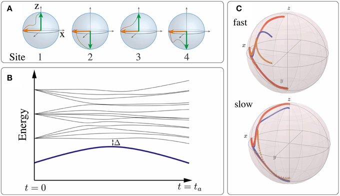
Figure 1. (A) In the adiabatic quantum optimization protocol, the system (depicted: four spins represented by their Bloch spheres) is prepared in a known ground state of the simple Hamiltonian H_init (orange arrows pointing to the left). The system is then transferred to the final Hamiltonian H_final with the ground state, given by the green arrows, that is the solution of the optimization problem. (B) If the transformation is performed adiabatically and shielded from decoherence effects, the system remains in the instantaneous ground state (thick blue) protected by the gap Δ. (C) Evolution of the state vectors of four spins (indicated by different colors) on the Bloch sphere for a typical choice of interactions J_ij. For slow annealing (t_a = 512/J, bottom), the protocol does reach the final ground state at the poles of the Bloch sphere, while it fails to do so for fast annealing (t_a = 64/J, top).

The AQO scheme becomes particularly appealing for complex problems where H_final is characterized by a high roughness of the free-energy landscape. Such problems are equivalent to spin glasses, where classical annealing is known to experience a dramatic slow down at low temperatures because energy barriers become exponentially large [32]. By overcoming the barriers via quantum tunneling [33] instead of thermal activation, quantum annealing as defined in Equation (2) offers the prospect of outperforming classical annealing [18]. However, the speed-up of quantum annealing has been only shown for certain classes of problems [19, 20] and for devices running at finite temperature AQO has been put into question entirely [30, 34]. In all of this, the precise role of quantum effects during the sweep is an open question, although the presence of entanglement during quantum annealing at finite temperature has recently been demonstrated in superconducting qubits [31].

A measure for the efficiency of AQO protocols is the success probability P, defined as the overlap between the final state |ψ(t_a)〉 with the actual ground state |ψ_gs〉 of H_final. Note that this measure can only serve as a benchmark, since it requires a priori knowledge about the solution of the problem. In addition, we also consider the instantaneous success probability P(t), which monitors the overlap of the state at time t with the desired final ground state, i.e.,

$\begin{array}{cc}P(t)=|\langle \psi (t)|{\psi }_{\text{gs}}\rangle {|}^2.& (3)\end{array}$

At the end of the protocol at time t = t_a, this quantity coincides with the success probability, P(t_a) = P.

Before presenting the results, we give a short overview of the structure of this paper. In Section 2, we present feasible implementations of various NP-complete problems in trapped ions and show how noise can be engineered in a controlled manner. In Section 3, we introduce relevant entanglement measures that we use in this work. Analytical results on the relation between entanglement after the sweep and the success probability are presented in Section 4. Numerical results for closed and open systems are discussed for a model problem, the Coulomb glass, in Section 5. We close by presenting our conclusions in Section 6.

2. Quantum Adiabatic Optimization with Trapped Ions

In this section, we present how current trapped-ion technology [6–13] can be extended to implement several well-known NP-complete problems [14, 15]. The main challenge is to encode these problems in H_final Equation (1), which requires a certain degree of programmability of interactions J_ij and fields h^z_i. Below, we present several models where a local variation of laser power is sufficient to obtain this programmability—as opposed to a much more difficult programming by, e.g., an extensive number of laser frequencies [35] or specially designed trapping potentials [36–39]. We also describe how engineered noise can be generated in order to study the interplay between decoherence, non-adiabaticity, and entanglement in the well-controlled architecture provided by trapped ions.

2.1. Ion Hamiltonian

We consider a chain of ions confined in a linear Paul trap. The spin-1/2 Ising variables appearing in H_final can be encoded by restricting the internal atomic dynamics to only two hyperfine sublevels. Single-qubit rotations allow for a preparation with high fidelity of any desired initial product state [13], including the completely polarized ground state of H_init [6–8, 10–13]. Similarly, the projection of the spin-1/2 variable on any coordinate direction can be measured to high precision by appropriate single-qubit rotations followed by stimulated fluorescence measurements, allowing the reconstruction of arbitrary correlation functions [7, 13]. The synthetic magnetic fields h^z_i and h^x appearing in H_final and H_init can also be simulated in a straightforward fashion via AC-Stark shifts or by resonantly driving the transition between the two sublevels [40].

Ising interactions can be simulated by coupling the ions via laser [40–42] or microwave radiation [43] to the collective vibrational modes. In the limit of off-resonant radiation, one can disentangle the collective vibrations and the atomic Ising variables via a canonical transformation and obtain an effective Hamiltonian for the Ising variables alone. For example, when employing a Mølmer–Sørensen scheme [42], the Ising spins are subject to the effective interactions (see Appendix A)

$\begin{array}{cc}{J}_{ij}=-\hslash \frac{|{\Omega }_i||{\Omega }_j|}{4}{\displaystyle \sum _q\frac{{\eta }_{iq}{\eta }_{jq}}{{\delta }_q}},& (4)\end{array}$

where η_iq is Lamb–Dicke parameter including the amplitude of vibrational mode q at ion i, δ_q is the detuning of the laser relative to the vibrational mode q, and |Ω_i| is the absolute value of the laser's Rabi frequency at ion i. For the derivation of Equation (4), we assumed the off-resonance condition η_iq|Ω_i| ≪ δ_q. The addition of a transverse field, required for our choice of H_init, induces additional couplings to the phonon modes in higher order, which, however, can be neglected as long as h^ν_i ≪ ħδ_q, ν = x, z. The precise form of the interactions depends on the coupling scheme used, but the qualitative behavior is similar for other schemes [40, 43].

As shown, e.g., in Britton et al. [10], Islam et al. [8], Jurcevic et al. [13], when transmitted via the transverse phonon modes the Ising interactions follow an approximate power law as a function of the distance, J_ij ~ 1/|i−j|^α, with a decay coefficient 0 ≤ α ≤ 3 that can be adjusted using the detuning δ_q (where larger detuning entails larger α). When employing the longitudinal phonon modes, the large spacing of vibrational frequencies restricts the range to α ≈ 0. By expressing the local Rabi frequencies as multiplies of a reference frequency |Ω|, i.e., |Ω_i| = F_i|Ω|, we can thus write

$\begin{array}{cc}{J}_{ij}=J\frac{F_i{F}_j}{|i-j{|}^{\alpha }},& (5)\end{array}$

with J setting the overall energy scale. Note that the power-law decay is exact only in the limits α = 0 and α = 3. As shown recently in Karp [44], the interactions in the intermediate regimes are better described by an exponential tail added to a dipolar decay. Additional modifications may arise from an uneven spacing of ions as is usual in linear Paul traps or from inhomogeneous laser profiles. For small chains, a general power-law behavior is, however, a good approximation of the system dynamics [13].

Until now, we considered a coupling to a single set of vibrational modes. However, richer models can be quantum simulated by employing the fact that in a linear Paul trap the three orthogonal directions of vibration decouple [40]. In this case, by using different lasers to couple to each orthogonal set of modes, it is possible to generate three independent Ising interaction terms, which we label ℓ = 1, 2, 3. Additionally, one may induce synthetic fields h^z_i in an ion-dependent fashion by, e.g., resonantly driving the qubit transitions with beams derived from an acousto-optic deflector [13]. It is thus possible to realize in trapped ions—using available technology—the following Ising Hamiltonian:

$\begin{array}{cc}{H}_{\text{final}}={\displaystyle \sum _{\ell =1,2,3}J}{\displaystyle \sum _{i\ne j}\frac{F_i^{(\ell )}{F}_j^{(\ell )}}{{\left|i-j\right|}^{{\alpha }^{(\ell )}}}}{\sigma }_i^z{\sigma }_j^z+{\displaystyle \sum _i{h}_i^z}{\sigma }_i^z.& (6)\end{array}$

2.2. NP-Complete Models Realizable with Available Trapped-Ion Technology

Experiments thus far—aiming at mimicking translationally invariant many-body models—made great efforts to engineer systems as homogeneous as possible, i.e., F^(ℓ)_i = 1 and h^z_i = h^z, ∀i [7, 8, 10, 12, 13]. For the same reason, few theoretical works have considered a site-dependent tunability of couplings [38, 45–47] or fields [48]. In contrast, our purpose of engineering NP-complete problems in Hamiltonian Equation (1) requires a certain degree of programmability of the interaction matrix elements J_ij and fields h^z_i (see e.g., Lucas [16]). In Table 1, we present several NP-complete problems that can be implemented with interactions of the form given in Equations (5) and (6), i.e., without requiring a full programmability of interactions. These problems thus become amenable to current trapped-ion technology by adjusting the local laser intensities |Ω_i|².

TABLE 1

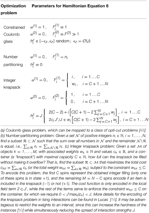
Table 1. NP-complete problems encodable via Hamiltonian Equation 6.

The NP-complete problems implementable in this way include the number-partitioning problem, the integer knapsack problem [16], and the Coulomb glass problem, which—as shown in Anjos et al. [49]—can be mapped to a class of opti-cut problems. We summarize the description of the necessary Hamiltonian parameters in Table 1. In the numerical studies presented in Section 5, we focus on the example of the Coulomb glass problem, since it is closest to current experiments [12, 13]. The Coulomb glass [51] contains a random magnetic field h^z_i ∈ [−ϵ_z, ϵ_z] and Ising interactions that are homogeneous and long-ranged, α⁽¹⁾ = 1 and F⁽¹⁾_i ≡ 1. Usually, one imposes the constraint of vanishing total magnetization, which can be realized by mean-field-like interactions (α⁽²⁾ = 0) with F⁽²⁾_i ≡ F⁽²⁾ ≫ 1. Defining the strength of the constraint as V ≡ J(F⁽²⁾)² ≫ J, the total Hamiltonian is then

$\begin{array}{cc}{H}_{\text{final}}=J{\displaystyle \sum _{i\ne j}\frac{{\sigma }_i^z{\sigma }_j^z}{|i-j|}}+{\displaystyle \sum _i{h}_i^z}{\sigma }_i^z+V{\displaystyle \sum _{i\ne j}{\sigma }_i^z}{\sigma }_j^z,& (7)\end{array}$

with J, V > 0. The large frustration of the Ising interactions counteracts ordering tendencies and, for ϵ_z = (J), leads to a strong competition between the interactions and the random local fields. This competition signs responsible for its computational complexity. Currently, it is not clear whether the Coulomb glass exhibits a spin-glass transition at nonzero temperature. This, however, does not necessarily imply a reduced complexity of the ground state of the model. Certain random Ising models on Chimera graphs, such as implemented in the D-Wave device, for example, do not show spin-glass transitions at nonzero temperature, but finding the ground state of the model is still NP-hard. Additionally, it may be that a non-perfect power-law decay, for example the more realistic dipolar plus exponential shape [44] affects the complexity of the model.

2.3. Noise Engineering

A fundamental question in AQO is how the optimization of problems such as given in Table 1 performs in the presence of decoherence. This question is of particular importance for current implementations of AQO devices such as the D-Wave machine where decoherence rates are large compared to the annealing times. Current trapped-ion setups are able to suppress noise to very low values, currently with time scales around 10/J [13]. This opens the possibility to systematically study the performance of AQO under varying degrees of purposefully engineered decoherence. A scheme to engineer different types of classical noise in a controlled fashion has recently been discussed and implemented in Soare et al. [52].

Here, we describe how classical white noise can be engineered by a conceptually simple extension of the steps leading up to Equation (4). Detailed derivations can be found in the Appendix C. Here, we sketch the main idea, which is based on the addition of randomly fluctuating synthetic magnetic fields. We assume that the rate of these fluctuations is much larger than any other parameter in the Hamiltonian, so that we can treat the annealing parameter A as quasi-constant. The total Hamiltonian then takes the form

$\begin{array}{cc}H=A{H}_{\text{init}}+(1-A)H_{\text{final}}+{\displaystyle \sum _i\left[{\xi }_i^x(t){\sigma }_i^x+{\xi }_i^z(t){\sigma }_i^z\right]},& (8)\end{array}$

where we choose the noise in two spin directions ν = x, z, and we take ξ^ν_i(t), to be independent Ornstein–Uhlenbeck processes, $\langle \langle {\xi }_i^{\nu }(t){\xi }_j^{\mu }(0)\rangle \rangle =\hslash \Gamma {\delta }_{\nu ,\mu }{\delta }_{i,j}\hslash b{\text{e}}^{-b\left|t\right|}$. Here, $\langle \langle ·\rangle \rangle$ denotes the average over noise realizations, and for simplicity we take the rate Γ and the bandwidth b to be independent of ν = x, z. The fluctuating fields can be realized using the same experimental techniques as for their quasi-static counterparts described at the beginning of Section 2.1. The additional requirement of fast fluctuations that are uncorrelated between different sites could be solved via a simultaneous addressing of the individual ions using several laser beams derived from an acousto-optic deflector [13].

If the bandwidth b of the fluctuations is much larger than the internal energy scales of the ions and the coupling to the phonon modes, b ≫ h^ν_i/ħ, η_iq|Ω_i|, we can average over the noise and obtain a master equation describing classical white-noise dephasing,

$\begin{array}{cc}\frac{\partial \rho }{\partial t}=-\frac{i}{\hslash }[H,\rho ]+\Gamma {\displaystyle \sum _{i}D}[{\sigma }_i^{(x)}]+\Gamma {\displaystyle \sum _{i}D}[{\sigma }_i^{(z)}],& (9)\end{array}$

where D[X] = 2XρX^† − ρX^†X − X^†Xρ is the Lindblad super-operator. In the derivation of Equation 9, we neglected additional couplings to the phonon modes that appear in higher order and can be dropped provided b ≫ η_iq|Ω_i|,h^ν_i/ħ. These conditions complement the requirements for the derivation of AH_init + (1 − A)H_final, which read δ_q ≫ η_iq|Ω_i|, h^ν_i/ħ. In the Appendix C, we discuss that they can all be fulfilled for realistic experimental parameters.

Hence, adding fluctuating fields with bandwidth much larger than other relevant energy scales allows to systematically engineer white noise in trapped ions. By inducing such fluctuations on the longitudinal or transversal fields, it is possible to study different types of Lindblad super-operators.

3. Entanglement Observables

AQO aims at solving classical problems using a quantum device, prompting the fundamental question of the role and importance of quantum effects within such a computational scheme. One particular feature of quantum as opposed to classical systems is entanglement, a theoretical study of which is the second central aim of this work. For that purpose, we use different quantifiers for quantum many-body correlations: the entanglement entropy, the logarithmic negativity, an optimal local entanglement witness, and the Fisher information. All of these quantifiers are sensitive toward different forms of entanglement and thus allow to address different aspects of entanglement.

In a perfect adiabatic protocol, entanglement vanishes in the initial and the final state, but it is finite during the sweep. The intermediate entanglement is due to avoided crossings between the ground state and excited states. In an optimal sweep, the final state shows no entanglement at all, as the true ground state is that of a classical Ising model. Therefore, entanglement in the final state is an indication for imperfections during the sweep. This mechanism of build-up and release of entanglement during an adiabatic optimization is the focus of the remainder of this work.

A full study of the many-body entanglement, which would require a full state tomography, is computationally and experimentally not feasible for all but very small systems. However, one can gain insight into different aspects of the problem from the combination of several entanglement measures and witnesses. In this chapter, we will give an overview of the various entanglement observables that we use. We also introduce a novel witness that can be efficiently measured in experiment.

3.1. Entanglement Entropy

A convenient, well-established measure for entanglement of closed systems is the entanglement entropy, which is defined between two subsystems A and B. The entanglement entropy is the von Neumann entropy of the reduced density matrix ρ_A = tr_Bρ of A obtained by tracing out the complement B,

$\begin{array}{cc}{S}_A=-\text{tr}\left[{\rho }_{\text{A}}\log ({\rho }_{\text{A}})\right].& (10)\end{array}$

In this work, we study the maximum of the entanglement entropy considering all possible pairs of particles as subsystem A and the remaining N − 2 particles as subsystem B. This pair-block entanglement entropy maximized over all pairs is denoted as S^max₂(t). The largest pair-block entanglement entropy reached during the sweep is S^max₂ = max_t [S^max₂(t)].

3.2. Logarithmic Negativity

A convenient mixed-state entanglement measure is the logarithmic negativity between two parts C and D of a larger subsystem A (A = C ∪ D). It is defined as [53, 54]

where $||X||=\text{tr}\sqrt{X^{†}X}$ is the trace norm. ρTCA is the partial transpose of the reduced density matrix ρA with respect to subpart C, given by 〈dc|ρTCA|d′c′〉 = 〈dc′|ρA|d′c〉 where the c's and d's form a basis for C and D, respectively. In the following, we consider the logarithmic negativity between subsystems C and D consisting of a single site each, and maximize again over all combinations.

3.3. Fisher Information

While entropy and negativity are measures for the entanglement between two subblocks of the system, we are also interested in multi-particle entanglement. This can be measured with the Fisher information F_Q, which not only quantifies entanglement, but also provides a lower bound on the number of particles that are entangled [55, 56]: if a state is k-producible—meaning that it can be written as a product of states involving less than or equal to k particles each—the Fisher information satisfies

$\begin{array}{cc}{F}_Q\le \lfloor \frac{N}{k}\rfloor k^2+{\left(N-\lfloor \frac{N}{k}\rfloor k\right)}^2.& (12)\end{array}$

Here, N is the total number of spins and ⌊ · ⌋ denotes the floor operation. If F_Q > N, this inequality implies entanglement between an increasing number of particles with increasing F_Q, where F_Q close to the maximal value of N² corresponds to N-particle entanglement. In quantum annealing devices, the multi-particle nature of entanglement may be a crucial aspect, since in a spin glass, for example, the lowest-energy configurations are typically vastly different. Thus, many spin flips should be necessary to tunnel from one local energy minimum to the next. If one assumes that all of these spins have to be coherent during the tunneling process, multi-particle entanglement may become the critical phenomenon for the efficiency of AQO protocols.

3.4. Optimal Local Entanglement Witness

While the above entanglement observables are powerful tools to theoretically understand the nature of entanglement, they require elaborate measurements in experiment. Therefore, it is desirable to find entanglement witnesses that can be deduced from simple observables.

Here, we introduce an optimal local entanglement witness W that allows one to measure entanglement in closed as well as open systems. It can be obtained from two-point spin correlations,

$\begin{array}{cc}W=\max \left\{0,-\underset{\overrightarrow{f}}{\min }\left[W_{\overrightarrow{f}}\right]\right\},& (13)\end{array}$

with

where f_i ∈ ℂ is subject to the normalization ∑_i|f_i|² = 1. This constitutes a generalization of the witnesses introduced in Krammer et al. [57], Cramer et al. [58], De Chiara and Sanpera [59], Hauke et al. [60]. Going beyond Hauke et al. [60], we analyze here the “optimal” witness, obtained by minimizing W_{$\overrightarrow{f}$} over all $\overrightarrow{f}$. In practical terms, this minimization is extremely simple: by introducing a Lagrange multiplier for the condition of normalization ∑_i|f_i|² = 1, it becomes equivalent to finding the smallest eigenvalue of the correlation matrix _ij = ${\displaystyle {\sum }_{\nu }\langle {\widehat{\sigma }}_i^{\nu }{\widehat{\sigma }}_j^{\nu }\rangle }$. This procedure can be done via post-processing of the measured two-point correlation functions, which are simple observables in trapped-ion experiments [6–13]. Thus, it is straightforward to determine the optimized entanglement witness experimentally. Since no cross-correlations of the form $\langle {\widehat{\sigma }}_i^x{\widehat{\sigma }}_j^y\rangle$ are required, it needs only three series of measurements for the x, y, and z correlations respectively, and is therefore easily scalable.

The above entanglement witness gives a lower bound on the best separable approximation (BSA) [58], an entanglement measure that is applicable also to mixed states. The ease of measuring this witness, both in theory and experiments, may make it an important entanglement quantifier, especially for large systems.

4. Upper Bound on the Efficiency from Entanglement

At the end of an ideal adiabatic protocol, the system arrives at the desired solution of the classical problem with vanishing entanglement. In presence of imperfections such as a non-adiabatic transfer of state population to higher energies, however, the final state will contain contributions from several eigenstates of H_final and in consequence a nonzero entanglement. It is the aim of this section is to show that it is possible to quantify this connection between entanglement and success probability in terms of the following bound

$\begin{array}{cc}{S}_l^{\text{end}}\le -P\log (P)-(1-P)\log (1-P)+(1-P)\log (2^l-1),& \left(15\right)\end{array}$

valid for P > 1/e with e Euler's number. Here, S^end_l denotes the final entanglement entropy of an arbitrary subsystem containing l spins. Remarkably, although S^end_l and P depend on the microscopic details of the system, the bound itself is independent of any microscopic parameters and as such completely universal. Below, we will show numerical data demonstrating that in most cases there is at least one subblock of l = 2 spins where the bound is closely approached as long as the sweep is sufficiently adiabatic.

We now prove the bound Equation (15). Let us denote the desired solution of the ideal problem by the spin configuration

$\begin{array}{cc}|s^{\ast }\rangle =|s_A^{\ast }{s}_B^{\ast }\rangle ,& \left(16\right)\end{array}$

where |s*_A/B〉 denotes the spin configurations in the respective subsystems A and B. This product form of the desired solution is always possible because the ground state |s*〉 of the classical Hamiltonian H_final is a separable state.

In a non-adiabatic sweep, the final reduced density matrix ρ_A of subsystem A will contain diagonal as well as off-diagonal elements. Let us denote by ρ^d_A the diagonal part of the original density matrix ρ_A, i.e., where all off-diagonal elements in the σ^z-basis are set to zero. The associated so-called diagonal entropy S^d_A satisfies the inequality [61]

$\begin{array}{cc}{S}_A\le S_A^d=-\text{tr}[{\rho }_A^d\log ({\rho }_A^d)]=-{\displaystyle \sum _{\mu =1}^{d_A}{p}_{\mu }}\log (p_{\mu }).& \left(17\right)\end{array}$

Here, p_μ denote the eigenvalues of ρ^d_A and d_A = 2^l is the size of the Hilbert space of the subblock A consisting of l spins. The magnitude of the diagonal elements can be estimated in the following way. Consider the matrix element p₁ defined as

$\begin{array}{cc}{p}_1=\langle s_A^{\ast }|{\rho }_A^d|s_A^{\ast }\rangle ={\displaystyle \sum _{\nu }\langle s_A^{\ast }\nu |\rho |s_A^{\ast }\nu \rangle }\ge P.& \left(18\right)\end{array}$

The matrix element p₁ is the probability to be locally in the ground state, i.e., all spins of the block A are oriented in the direction of the desired solution, Equation (16), and ν sums over all spin configurations of the complement B. The inequality in the above Equation (18) follows because all diagonal elements of the density matrix ρ are nonnegative. When P ≥ 1/e, i.e., for not too small success probabilities, Equation (18) gives −p₁ log(p₁) ≤ −Plog(P), and inequality (17) becomes

$\begin{array}{cc}{S}_A\le -P\log (P)-{\displaystyle \sum _{\mu =2}^{d_A}{p}_{\mu }}\log (p_{\mu }).& \left(19\right)\end{array}$

The contribution to the diagonal entropy from the states other than the local ground state assumes its maximum for the case of equipartitioned probabilities, p_μ = C/(d_A − 1), with μ ≥ 2 and C a constant. The normalization of the density matrix imposes the constraint ${\displaystyle {\sum }_{\mu =1}^{d_A}{p}_{\mu }}=1=p_1+C$. Using p₁ ≥ P, this gives C ≤ 1 − P, which implies

$\begin{array}{cc}-C\log (C)\le -(1-P)\log (1-P).& \left(20\right)\end{array}$

For a subblock A consisting of l spins, this directly gives the desired upper bound in Equation (15) by denoting S_A as S^end_l.

An important application of the bound is an estimation of the success probability from entropy measurements with polynomial effort in system size. A direct measurement of the success probability requires knowledge of the desired solution, the exponentially hard problem we set out to solve in the first place. However, the entanglement entropy of a subblock of small size, l = 2 say, only requires mapping out the reduced density matrix of l spins. This can be performed efficiently even though the total number of spins N might be very large. The maximization over all sets of fixed size l = 2 leads to an additional increase of measurement resources, but it remains polynomial because the total number of partitions into subblocks of e.g., size l = 2 is N(N − 1)/2.

5. Numerical Results

We now study numerically the interrelation between entanglement, success probability, and decoherence in the Coulomb-glass problem, Equation (7). In particular, we show that the bound Equation (15) is a useful measure for the success probability. As initial state of the AQO protocol, we choose the ground state of H_init = h^x ∑_iσ^x_i, a classical product state, and we employ a linear ramp, i.e., A(t) = 1 − t/t_a. Note, that possible optimized non-linear ramps may improve the performance of the AQO protocol [19, 62]. We use ϵ_z/J = 1/2 and V/J = 10 as system parameters. Before turning to open systems described by the master Equation (9), it is instructive to understand the decoherence-free case, which is the subject of the following section.

5.1. Closed Quantum Systems

For computing the dynamics in closed systems, we employ exact diagonalization with Krylov time evolution [63] for N = 16 spins, and with about 100 disorder realizations of h^z_i for each value of t_a. Note, that the focus of this work is the entanglement during the optimization with restricts the number of spins to relatively small sizes.

Let us first illustrate the dynamics of the entanglement in typical sweeps. Figure 2 depicts the entanglement dynamics and success probability of a few instances of randomly chosen magnetic fields h^z_i. In these examples, the annealing time is fixed to a moderate value t_a = 500/J, such that for most instances the sweep is nearly adiabatic (here, as in what follows, we set ħ to unity). Starting from the separable initial state, entanglement gradually increases up to a maximum around t/t_a ≈ 0.6 − 0.7, i.e., in the vicinity of the equilibrium magnetic phase transition of the homogeneous system. During the final stages of the protocol, the quantum fluctuations introduced via the transverse fields h^x ∑_i σ^x_i become weaker; the entanglement decays while simultaneously the success probability increases. There exist, however, particular “hard” instances where the system is not capable to disentangle, and thus ends up in a superposition of various eigenstates with a lower success probability. The optimal local entanglement witness, which is not an entanglement measure, shows stronger oscillations than the other observables, which results in a peculiar additional peak in the hard instance of Figure 2.

FIGURE 2

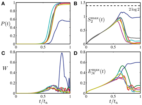
Figure 2. Success probability (A) and entanglement dynamics (B–D) during the adiabatic quantum optimization protocol, for a few instances (shown in different color) of randomly drawn magnetic fields h^z_i ∈ [−ϵ_z, ϵ_z], with ϵ_z/J = 1/2. System size is N = 16, for which the chosen annealing time t_a = 500/J is a moderate value. (A) The instantaneous success probability, i.e., the overlap with the solution of the optimization problem, increases strongly in the vicinity of the equilibrium magnetic phase transition of the homogeneous system. (B) Dynamics of the entanglement entropy S^max₂(t) of two spins with the rest, (C) the optimal local entanglement witness W, and (D) the logarithmic negativity E^max(t) between pairs of spins. Both S^max₂(t) and E^max(t) have been obtained by maximization over all possible permutations of two sites on the chain. Easy instances [large P(t_a)] are able to reduce the entanglement obtained around the equilibrium phase transition, while hard instances (blue) remain strongly entangled even toward the end of the protocol.

5.1.1. Final-State Entanglement

We will now quantitatively analyze these observations, starting with the final entanglement at t = t_a. Figure 3, upper row, depicts the final entanglement S^end₂ ≡ S^max₂(t_a) as a function of P for various annealing times t_a. The smaller t_a the more excitations are created during the sweep. The result is an effective heating that leads to an increased entanglement entropy at the end of the protocol. At the same time, the generated excitations induce a substantial loss of success probability.

FIGURE 3

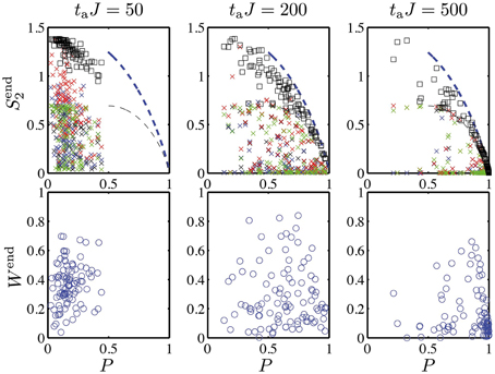
Figure 3. Success probability as a function of final entanglement for different annealing times t_a, in a closed system (parameters as in Figure 2). Top: Final entanglement entropy S^end₂ of exemplary subsystems of size 2 (crosses). The different colors denote entanglement of the following subsystems with the rest of the chain: {1, 2} (black), {1, 3} (blue), {1, 16} (red), and {12, 14} (green). When maximized over all possible subsystems containing two sites (black squares), the entanglement entropy lies close to the theoretical upper bound Equation (15) (blue dashed line). The thin black dashed line is the bound for a subsystem of length l = 1. Bottom: The optimized entanglement witness shows a qualitatively similar behavior as the entanglement entropy S^end₂ of typical subsystems. Compared to the maximized S^end₂, however, W^end shows a larger number of instances with small entanglement, indicating that it does not capture all entanglement present in the system. As a result, correlations between success probability and W^end are washed out.

At small annealing times, the qubit pair with maximal entanglement entropy approaches S^end₂ = 2log 2, the von Neumann entropy of an infinite-temperature state.

For larger annealing times t_a = 500/J, on the other hand, the maximally entangled qubit pair approaches the bound in Equation (15) for many instances, implying that the system achieves the maximally possible success probability given the entropy of the state. Thus, in this regime it is possible to estimate the success probability, an exponentially hard problem, from purely local measurements involving only resources scaling polynomially with system size, as discussed in Section 4. But notice that even for these moderate annealing times there are still hard instances with a small success probability and an associated large final entanglement.

In Figure 3, lower row, we compare the optimal local entanglement witness with the entanglement entropy. The witness W^end reproduces the features of the entanglement entropy of typical subsystems but not of the maximized entanglement entropy S^end₂. For fast sweeps, the optimal witness in the final state approaches W ≈ 1/2, which corresponds to its infinite-temperature value, suggesting a strong heating of the system. Increasing the sweep time reduces the final entanglement for most instances. These findings are analogous to the behavior of the entanglement entropy.

For the logarithmic negativity, we find a behavior that is qualitatively similar to the optimal witness. As seen in Figure 4, the optimal witness provides a rough lower bound for the logarithmic negativity: a large W results in a large E, but not necessarily vice versa. Although the entanglement witness W^end, therefore, can provide a useful operational measure to evaluate the entanglement in the annealing procedure, it shows quantitative differences to more complex entanglement measures. Its shortcomings are clearly seen in some instances that fail to disentangle the state toward the end of the time evolution, where we find strong oscillations in the witness (see Figure 2), which, however, are not accompanied by a further feature in either the entanglement entropy or the logarithmic negativity.

FIGURE 4

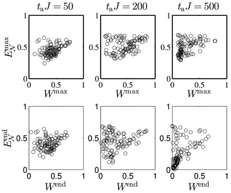
Figure 4. Logarithmic negativity E compared to the optimized entanglement witness W, for different annealing times t_a in a closed system of N = 16 sites. Top: Comparison of maximal values during the annealing procedure. Bottom: final values. W provides a rough lower bound for E. While the tendency for these entanglement observables, is to become smaller with increasing t_a, in particular for the final values, correlations to the success probability are difficult to find: for all considered annealing times, both quantities have a broad available range of maximal and final values.

5.1.2. Maximal Entanglement

From the entanglement entropy, and in particular the bound given in Equation (15), we found a small entanglement in the final state is crucial for the efficiency. However, the maximal entanglement achieved during the sweep does not seem to be much correlated with the success probability, as can be seen in Figure 5, where we display the behavior of the entanglement entropy S^max₂ = max_t [S^max₂(t)] (again maximized over all subblocks with l = 2) as well as the witness W^max = max_t W(t).

FIGURE 5

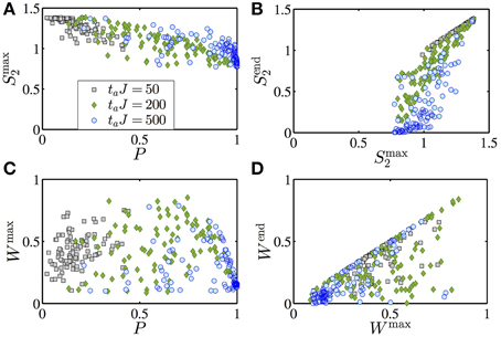
Figure 5. Maximal entanglement reached during the optimization algorithm in closed systems of N = 16 sites for different annealing times t_aJ = 50 (black squares), 200 (green diamonds) and 500 (blue lozenges). (A) Entanglement entropy between two sites and the rest of the system, maximized over all pairs of sites, and (C) optimized entanglement witness, both as a function of success probability. The measured entanglement occupies a broad range, making it difficult to find correlations to the success probability. The maximal entanglement entropy shows only a slight anticorrelation with the success probability P, which is inherited from the bound Equation (15) and the fact that the final-state entropy for unsuccessful sweeps remains close to the maximal one (B). This behavior is less prominent for the entanglement witness (D).

For large annealing times, the maximal entanglement entropy and witness are spread over a large range of values. This makes it difficult to draw a correlations with the success probability. For faster sweeps, there is a slight anticorrelation between S^max₂ and P, but this derives from the bound Equation (15), since then the maximal entanglement is retained at the end of the protocol. This can be appreciated in Figures 5B,D, where it is seen that, for fast annealing, the entanglement at the end is similar to the maximal entanglement. In these figures, one can also see that for slower sweeps, i.e., for more successful instances, the final entanglement is considerably lower than the one attained at the maximum. The logarithmic negativity presents a qualitatively similar behavior (not shown).

In conclusion, we find no useful correlations between maximal entanglement during the sweep and success probability. In particular, instances that experience a large entanglement during the sweep do not show a larger success probability—contrary to what one might expect when considering the popular picture of spin configurations that quantum tunnel through energy barriers.

5.2. Open Quantum Systems

In an ideal, closed system, the only mechanism to lower the success probability is non-adiabaticity due to finite sweeping times. However, in many current implementations of AQO, the efficiency is also reduced by decoherence in the system. In particular, in the D-wave device, decoherence is orders of magnitude faster than annealing times. Trapped ions, on the other hand, operate in a regime where, as we have shown in Section 2, decoherence can be systematically tuned. This ability allows one to study the complex interplay between non-adiabaticity and decoherence in AQO. In this section, we numerically analyze entanglement witness W, negativity E and the Fisher information F_Q in the AQO protocol. We present numerical data from a relatively small system with N = 6 sites where considerable statistics is achievable also for numerically exact open-system calculations. In current experiments, the number of ions can go up to N = 20 [5], which represents an example of a quantum simulator reaching system sizes that cannot be sampled numerically.

We compare various annealing times t_a, ranging from t_a = 4/J to t_a = 256/J, and decoherence rates ranging from Γ = 0 to Γ = 0.01J, depicted in Figure 6. For fast sweeps (t_a = 4/J), the results are independent of Γ, as can be expected since the considered rates are too low to have any effect in this case. In this regime, the final state remains close to the initial equal superposition of all eigenstates of the final Hamiltonian, and the success probability approaches the limit of P = 1/2^N, independent of the rate of decoherence. The entanglement in the final state is then rather uncorrelated from the success probability, which is always low.

FIGURE 6

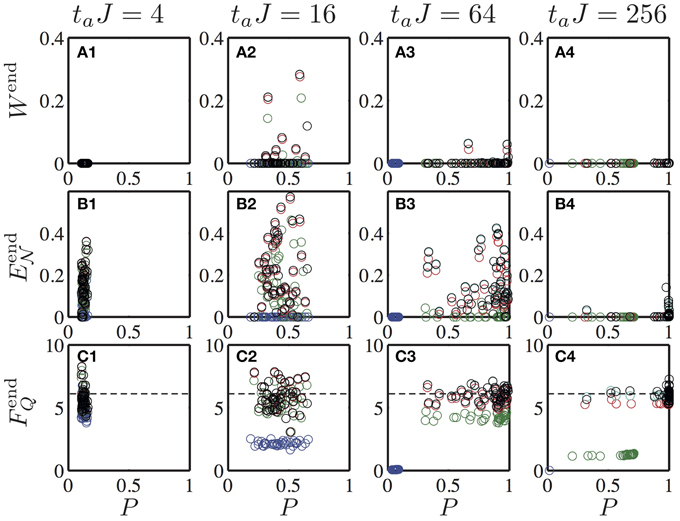
Figure 6. Scatter plot of success probability P against the witness (top), logarithmic negativity (middle), and Fisher information (bottom) for N = 6 spins. Colors indicate the decoherence rate, ranging from Γ = 0 (black), Γ = 0.0001J (red), Γ = 0.001J (green), to Γ = 0.01J (blue). For small t_a, the final state is always close to an equal superposition of all eigenstates with a small success probability. Fisher information and logarithmic negativity show some residual entanglement. At large t_a, the success probability decreases with increasing decoherence rate, which also suppresses logarithmic negativity and Fisher information. The dashed line marks F_Q = N, above which the system hosts entanglement.

In the opposite extreme of slow sweeps (t_a = 256/J), the success probability P is governed almost solely by the decoherence rate, and, contrary to the case of closed systems, has little relation to the final-state entanglement. In fact, in this case of extremely slow sweeps, only at small decoherence does any entanglement as measured through E and F_Q survive, while the witness W vanishes for all studied instances. In the regime of intermediate annealing times, for small decoherence rates the success probability and entanglement are related in a similar fashion as in the fully coherent case, but a large decoherence suppresses both entanglement and success probability.

The optimal witness is rather sensitive to decoherence and does not allow one to obtain detailed information about the process. In contrast, the Fisher information shows rich features and offers additional insight into the nature of the entanglement of the final state. The cases of slow sweeps (t_a = 256/J) and small decoherence rates are particularly interesting for the AQO protocol, since these allow for a large success probability. In these cases, we find that the Fisher information approaches F_Q ≈ N, which indicates entanglement with k ≈ 1, i.e., between individual particles. For faster annealing, F_Q can increase slightly, but still remains much below F_Q = N². We find a similar behavior for the maximum of F_Q assumed during the AQO sweep. This means entanglement between large numbers of particles as measured through F_Q is rare for the studied system sizes.

State-of-the-art trapped-ion experiments have intrinsic decoherence rates on the order of Γ ~ 0.1J, but predominantly only in one quadrature [13]. We have performed numerical tests also for dephasing only and found an improvement of a factor of about 2 compared to the results presented in Figure 6, where we considered the worst case of equal noise in σ^x and σ^z. Thus, for a systematic study of the influence of noise on AQO in such setups, further improvements in terms of decoherence still seem necessary. Also, as is usual with AQO protocols, larger problem instances will show smaller gaps and thus require larger annealing times to achieve similar degrees of success probability. On the other hand, non-linear ramps may improve the performance of the AQO protocol [19, 62].

6. Conclusions

In this work, we presented a feasible way to study the interrelation between entanglement, non-adiabaticity, and decoherence on small scales in a well-controlled laboratory setting. In particular, we proposed several NP-complete problems that can be implemented with straightforward extensions of existing trapped-ion architectures. We described how fluctuating synthetic fields allow to engineer well-controlled, artificial decoherence sources that take advantage of the low levels of natural decoherence. Further, we introduced an entanglement witness that is simple to measure in a scalable way, yet reproduces some of the main features of more complex entanglement measures, such as the entanglement entropy and the logarithmic negativity.

Using extensive numerically exact studies on small closed and open systems, we analyzed the dynamics of entanglement during adiabatic quantum optimization. We found that, contrary to popular assumption, a large entanglement during the optimization has little significance for its success probability. On the other hand, in clean systems, a large final entanglement after not too fast sweeps indicates that the sweep generated a superposition state as its outcome, with decreased probability to arrive in the separable ground state that solves the optimization problem. Decoherence diminishes this anticorrelation between final-state entanglement and success probability.

Thus, it seems that the simple presence or absence of entanglement does not allow to conclude on the efficiency of a machine performing adiabatic quantum optimization—at least in the case of the entanglement quantifiers and the systems considered in this article. It will be interesting to study whether such correlations appear for larger systems, optimized ramps, or other optimization problems. More work is clearly needed to understand if and how entanglement may sign responsible for a quantum speedup of adiabatic quantum optimization.

Conflict of Interest Statement

The authors declare that the research was conducted in the absence of any commercial or financial relationships that could be construed as a potential conflict of interest.

Acknowledgments

We acknowledge fruitful discussions with Andreas Läuchli and Peter Zoller. This work was supported by the EU integrated project SIQS, ERC synergy grant UQUAM, the Austrian Science Fund (FWF) through the SFB FoQuS (FWF Project No. F4016-N23), and the Austrian Ministry of Science BMWF as part of the UniInfrastrukturprogramm of the Research Platform Scientific Computing at the University of Innsbruck. WL acknowledges support by the Austrian Science Fund (FWF): P 25454-N27 and MH acknowledges support by the Deutsche Akademie der Naturforscher Leopoldina under grant number LPDS 2013-07. Bloch spheres in Figure 1 and master-equation calculations for open systems used the Qutip libraries [64].

References

1. Wineland DJ, Bollinger JJ, Itano WM, Moore FL, Heinzen DJ. Spin squeezing and reduced quantum noise in spectroscopy. Phys Rev A (1992) 46:R6797–800. doi: 10.1103/PhysRevA.46.R6797

PubMed Abstract | Full Text | CrossRef Full Text | Google Scholar

2. Johanning M, Varón AF, Wunderlich C. Quantum simulations with cold trapped ions. J Phys B (2009) 42:154009. doi: 10.1088/0953-4075/42/15/154009

PubMed Abstract | Full Text | CrossRef Full Text | Google Scholar

3. Blatt R, Roos CF. Quantum simulations with trapped ions. Nat Phys. (2012) 8:277. doi: 10.1038/nphys2252

CrossRef Full Text | Google Scholar

4. Schneider C, Porras D, Schaetz T. Experimental quantum simulations of many-body physics with trapped ions. Rep Prog Phys. (2012) 75:024401. doi: 10.1088/0034-4885/75/2/024401

PubMed Abstract | Full Text | CrossRef Full Text | Google Scholar

5. Monroe C, Kim J. Scaling the ion trap quantum processor. Science (2013) 339:1164. doi: 10.1126/science.1231298

PubMed Abstract | Full Text | CrossRef Full Text | Google Scholar

6. Friedenauer A, Schmitz H, Glueckert JT, Porras D, Schaetz T. Simulating a quantum magnet with trapped ions. Nat Phys. (2008) 4:757. doi: 10.1038/nphys1032

CrossRef Full Text | Google Scholar

7. Lanyon BP, Hempel C, Nigg D, Müller M, Gerritsma R, Zähringer F, et al. Universal digital quantum simulation with trapped ions. Science (2011) 7:57. doi: 10.1126/science.1208001

PubMed Abstract | Full Text | CrossRef Full Text | Google Scholar

8. Islam R, Senko C, Campbell WC, Korenblit S, Smith J, Lee A, et al. Emergence and frustration of magnetic order with variable-range interactions in a trapped ion quantum simulator. Science (2013) 340:583. doi: 10.1126/science.1232296

PubMed Abstract | Full Text | CrossRef Full Text | Google Scholar

9. Khromova A, Piltz C, Scharfenberger B, Gloger TF, Johanning M, Varón AF, et al. Designer spin pseudomolecule implemented with trapped ions in a magnetic gradient. Phys Rev Lett. (2012) 108:220502. doi: 10.1103/PhysRevLett.108.220502

PubMed Abstract | Full Text | CrossRef Full Text | Google Scholar

10. Britton JW, Sawyer BC, Keith AC, Wang C-CJ, Freericks JK, Uys H, et al. Engineered two-dimensional ising interactions in a trapped-ion quantum simulator with hundreds of spins. Nature (2012) 484:489. doi: 10.1038/nature10981

PubMed Abstract | Full Text | CrossRef Full Text | Google Scholar

11. Richerme P, Senko C, Korenblit S, Smith J, Lee A, Islam R, et al. Quantum catalysis of magnetic phase transitions in a quantum simulator. Phys Rev Lett. (2013) 111:100506. doi: 10.1103/PhysRevLett.111.100506

PubMed Abstract | Full Text | CrossRef Full Text | Google Scholar

12. Richerme P, Gong Z-X, Lee A, Senko C, Smith J, Foss-Feig M, et al. Non-local propagation of correlations in long-range interacting quantum systems. Nature (2014) 511:198. doi: 10.1038/nature13450

PubMed Abstract | Full Text | CrossRef Full Text | Google Scholar

13. Jurcevic P, Lanyon BP, Hauke P, Hempel C, Zoller P, Blatt R, et al. Observation of entanglement propagation in a quantum many-body system. Nature (2014) 511:202. doi: 10.1038/nature13461

PubMed Abstract | Full Text | CrossRef Full Text | Google Scholar

14. Karp R. Reducibility Among Combinatorial Problems, Complexity of Computer Computations, 85 Edn. New York, NY: Springer (1972).

15. Garey M, Johnson D. Computers and Intractability: A Guide to the Theory of NP-Completeness. New York, NY: W. H. Freeman and Company (1979).

16. Lucas A. Ising formulations of many NP problems. Front Phys. (2014) 2:5. doi: 10.3389/fphy.2014.00005

CrossRef Full Text | Google Scholar

17. Farhi E, Goldstone J, Gutmann S, Lapan J, Lundgren A, Preda D. A quantum adiabatic evolution algorithm applied to random instances of an NP–complete problem. Science (2001) 292:472. doi: 10.1126/science.1057726

PubMed Abstract | Full Text | CrossRef Full Text | Google Scholar

18. Santoro GE, Martonak R, Tosatti E, Car R. Theory of quantum annealing of an ising spin glass. Science (2002) 295:2427. doi: 10.1126/science.1068774

PubMed Abstract | Full Text | CrossRef Full Text | Google Scholar

19. Roland J, Cerf NJ. Quantum search by local adiabatic evolution. Phys Rev A (2002) 65:042308. doi: 10.1103/PhysRevA.65.042308

PubMed Abstract | Full Text | CrossRef Full Text | Google Scholar

20. Amin MHS, Love PJ, Truncik CJS. Thermally assisted adiabatic quantum computation. Phys Rev Lett. (2008) 100:060503. doi: 10.1103/PhysRevLett.100.060503

PubMed Abstract | Full Text | CrossRef Full Text | Google Scholar

21. Hen I. How fast can quantum annealers count? J Phys A (2014) 47:235304. doi: 10.1088/1751-8113/47/23/235304

CrossRef Full Text | Google Scholar

22. Heim B, Rønnow TF, Isakov SV, Troyer M. Quantum versus classical annealing of ising spin glasses. Science (2015) 348:215–17. doi: 10.1126/science.aaa4170

PubMed Abstract | Full Text | CrossRef Full Text | Google Scholar

23. Johnson MW, Amin MHS, Gildert S, Lanting T, Hamze F, Dickson N, et al. Quantum annealing with manufactured spins. Nature (2011) 473:194. doi: 10.1038/nature10012

PubMed Abstract | Full Text | CrossRef Full Text | Google Scholar

24. Perdomo-Ortiz A, Dickson N, Drew-Brook M, Rose G, Aspuru-Guzik A. Finding low-energy conformations of lattice protein models by quantum annealing. Sci Rep. (2012) 2:571. doi: 10.1038/srep00571

PubMed Abstract | Full Text | CrossRef Full Text | Google Scholar

25. Bian Z, Chudak F, Macready WG, Clark L, Gaitan F. Experimental determination of ramsey numbers. Phys Rev Lett. (2013) 111:130505. doi: 10.1103/PhysRevLett.111.130505

PubMed Abstract | Full Text | CrossRef Full Text | Google Scholar

26. Boixo S, Albash T, Spedalieri FM, Chancellor N, Lidar DA. Experimental sigNature of programmable quantum annealing. Nat Comm. (2013) 4:3067. doi: 10.1038/ncomms3067

PubMed Abstract | Full Text | CrossRef Full Text | Google Scholar

27. Boixo S, Ronnow TF, Isakov SV, Wang Z, Wecker D, Lidar DA, et al. Evidence for quantum annealing with more than one hundred qubits. Nat Phys (2014) 10:218. doi: 10.1038/nphys2900

CrossRef Full Text | Google Scholar

28. Steffen M, van Dam W, Hogg T, Breyta G, Chuang I. Experimental implementation of an adiabatic quantum optimization algorithm. Phys Rev Lett. (2003) 90:067903. doi: 10.1103/PhysRevLett.90.067903

PubMed Abstract | Full Text | CrossRef Full Text | Google Scholar

29. Altshuler B, Krovi H, Roland J. Anderson localization makes adiabatic quantum optimization fail. Proc Natl Acad Sci USA. (2010) 107:12446. doi: 10.1073/pnas.1002116107

PubMed Abstract | Full Text | CrossRef Full Text | Google Scholar

30. Rønnow TF, Wang Z, Job J, Boixo S, Isakov SV, Wecker D, et al. Defining and detecting quantum speedup. Science (2014) 345:420. doi: 10.1126/science.1252319

PubMed Abstract | Full Text | CrossRef Full Text | Google Scholar

31. Lanting T, Przybysz A, Smirnov AY, Spedalieri F, Amin M, Berkley A, et al. Entanglement in a quantum annealing processor. Phys Rev X (2014) 4:021041. doi: 10.1103/PhysRevX.4.021041

CrossRef Full Text | Google Scholar

32. Binder K, Young AP. Spin glasses: experimental facts, theoretical concepts, and open questions. Rev Mod Phys. (1986) 58:801. doi: 10.1103/RevModPhys.58.801

CrossRef Full Text | Google Scholar

33. Battaglia DA, Stella L. Optimization through quantum annealing: theory and some applications. Contemp Phys. (2006) 47:195–208. doi: 10.1080/00107510600861454

PubMed Abstract | Full Text | CrossRef Full Text | Google Scholar

34. Katzgraber HG, Hamze F, Andrist RS. Glassy Chimeras could be blind to quantum speedup: designing better benchmarks for quantum annealing machines. Phys Rev X (2014) 4:021008. doi: 10.1103/PhysRevX.4.021008

CrossRef Full Text | Google Scholar

35. Korenblit S, Kafri D, Campbell WC, Islam R, Edwards EE, Gong Z-X, et al. Quantum simulation of spin models on an arbitrary lattice with trapped ions. New J Phys. (2012) 14:095024. doi: 10.1088/1367-2630/14/9/095024

PubMed Abstract | Full Text | CrossRef Full Text | Google Scholar

36. Chiaverini J, Lybarger JWE. Laserless trapped-ion quantum simulations without spontaneous scattering using microtrap arrays. Phys Rev A (2008) 77:022324. doi: 10.1103/PhysRevA.77.022324

CrossRef Full Text | Google Scholar

37. Schmied R, Wesenberg JH, Leibfried D. Optimal surface-electrode trap lattices for quantum simulation with trapped ions. Phys Rev Lett. (2009) 102:233002. doi: 10.1103/PhysRevLett.102.233002

PubMed Abstract | Full Text | CrossRef Full Text | Google Scholar

38. Zippilli S, Johanning M, Giampaolo SM, Wunderlich C, Illuminati F. Adiabatic quantum simulation with a segmented ion trap: application to long-distance entanglement in quantum spin systems. Phys Rev A (2014) 89:042308. doi: 10.1103/PhysRevA.89.042308

CrossRef Full Text | Google Scholar

39. Wilson AC, Colombe Y, Brown KR, Knill E, Leibfried D, Wineland DJ. Tunable spin–spin interactions and entanglement of ions in separate potential wells. Nature (2014) 512:57. doi: 10.1038/nature13565

PubMed Abstract | Full Text | CrossRef Full Text | Google Scholar

40. Porras D, Cirac JI. Effective quantum spin systems with trapped ions. Phys Rev Lett. (2004) 92:207901. doi: 10.1103/PhysRevLett.92.207901

PubMed Abstract | Full Text | CrossRef Full Text | Google Scholar

41. Cirac JI, Zoller P. Quantum computations with cold trapped ions. Phys Rev Lett. (1995) 74:4091. doi: 10.1103/PhysRevLett.74.4091

PubMed Abstract | Full Text | CrossRef Full Text | Google Scholar

42. Sørensen A, Mølmer K. Quantum computation with ions in thermal motion. Phys Rev Lett. (1999) 82:1971. doi: 10.1103/PhysRevLett.82.1971

PubMed Abstract | Full Text | CrossRef Full Text | Google Scholar

43. Mintert F, Wunderlich C. Ion-trap quantum logic using long-wavelength radiation. Phys Rev Lett. (2001) 87:257904. doi: 10.1103/PhysRevLett.87.257904

PubMed Abstract | Full Text | CrossRef Full Text | Google Scholar

44. Nevado P, Porras D. Hidden frustrated interactions and quantum annealing in trapped ion spin-phonon chains. (2014) arXiv:1406.5094 [quant-ph].

Google Scholar

45. Bermudez A, Almeida J, Schmidt-Kaler F, Retzker A, Plenio MB. Frustrated quantum spin models with cold coulomb crystals. Phys Rev Lett. (2011) 107:207209. doi: 10.1103/PhysRevLett.107.207209

PubMed Abstract | Full Text | CrossRef Full Text | Google Scholar

46. Bermudez A, Almeida J, Ott K, Kaufmann H, Ulm S, Poschinger U, et al. Quantum magnetism of spin-ladder compounds with trapped-ion crystals. New J Phys. (2012) 14:093042. doi: 10.1088/1367-2630/14/9/093042

CrossRef Full Text | Google Scholar

47. Hauke P, Marcos D, Dalmonte M, Zoller P. Quantum simulation of a lattice Schwinger model in a chain of trapped ions. Phys Rev X (2013) 3:041018. doi: 10.1103/PhysRevX.3.041018

CrossRef Full Text | Google Scholar

48. Hauke P, Heyl M. Many-body localization and quantum ergodicity in disordered long-range ising models. (2014) arXiv:1410.1491 [cond-mat.dis-nn].

Google Scholar

49. Anjos MF, Liers F, Pardella G, Schmutzer A. Engineering branch-and-cut algorithms for the equicut problem. In: Bezdek K, Deza A, Ye Y, editors. Discrete Geometry and Optimization, Fields Institute Communications 69. Switzerland: Springer International Publishing (2013). p. 17–32.

50. Pisinger D. Where are the hard knapsack problems? Comput Oper Res. (2005) 32:2271. doi: 10.1016/j.cor.2004.03.002

CrossRef Full Text | Google Scholar

51. Ortuño M, Somoza AM. Coulomb Glasses. Lancaster University (2004). Available online at: http://www.lancaster.ac.uk/users/esqn/windsor04/docs/artuno-cg.pdf

52. Soare A, Ball H, Hayes D, Zhen X, Jarratt MC, Sastrawan J, et al. Experimental bath engineering for quantitative studies of quantum control. Phys Rev A (2014) 89:042329. doi: 10.1103/PhysRevA.89.042329

CrossRef Full Text | Google Scholar

53. Vidal G, Werner RF. Computable measure of entanglement. Phys Rev A (2002) 65:032314. doi: 10.1103/PhysRevA.65.032314

CrossRef Full Text | Google Scholar

54. Plenio MB. Logarithmic negativity: a full entanglement monotone that is not convex. Phys Rev Lett. (2005) 95:090503. doi: 10.1103/PhysRevLett.95.090503

PubMed Abstract | Full Text | CrossRef Full Text | Google Scholar

55. Hyllus P, Laskowski W, Krischek R, Schwemmer C, Wieczorek W, Weinfurter H, et al. Fisher information and multiparticle entanglement. Phys Rev A (2012) 85:022321. doi: 10.1103/PhysRevA.85.022321

PubMed Abstract | Full Text | CrossRef Full Text | Google Scholar

56. Pezzé L, Smerzi A. Entanglement, nonlinear dynamics, and the heisenberg limit. Phys Rev Lett. (2009) 102:100401. doi: 10.1103/PhysRevLett.102.100401

PubMed Abstract | Full Text | CrossRef Full Text | Google Scholar

57. Krammer P, Kampermann H, Bruss D, Bertlmann RA, Kwek LC, Macchiavello C. Multipartite entanglement detection via structure factors. Phys Rev Lett. (2009) 103:100502. doi: 10.1103/PhysRevLett.103.100502

PubMed Abstract | Full Text | CrossRef Full Text | Google Scholar

58. Cramer M, Plenio MB, Wunderlich H. Measuring entanglement in condensed matter systems. Phys Rev Lett. (2011) 106:020401. doi: 10.1103/PhysRevLett.106.020401

PubMed Abstract | Full Text | CrossRef Full Text | Google Scholar

59. De Chiara G, Sanpera A. Detection of entanglement in ultracold lattice gases. J Low Temp Phys. (2011) 165:292. doi: 10.1007/s10909-011-0403-8

CrossRef Full Text | Google Scholar

60. Hauke P, Sewell RJ, Mitchell MW, Lewenstein M. Quantum control of spin-correlations in ultracold lattice gases. Phys Rev A (2013) 87:021601(R). doi: 10.1103/PhysRevA.87.021601

CrossRef Full Text | Google Scholar

61. Polkovnikov A. Microscopic diagonal entropy and its connection to basic thermodynamic relations. Ann Phys. (2011) 326:486–99. doi: 10.1016/j.aop.2010.08.004

CrossRef Full Text | Google Scholar

62. Mandrà S, Guerreschi GG, Aspuru-Guzik A. Dimensionality reduction for adiabatic quantum optimizers: beyond symmetry exploitation. (2014) arXiv:1407.8183.

63. Park J-H, Light JC. Unitary quantum time evolution by iterative lanczos reduction. J Chem Phys. (1986) 86:5870. doi: 10.1063/1.451548

CrossRef Full Text | Google Scholar

64. Johansson J, Nation P, Nori F. QuTiP 2: a Python framework for the dynamics of open quantum systems. Comput Phys Commun. (2013) 184:1234–40. doi: 10.1016/j.cpc.2012.11.019

CrossRef Full Text | Google Scholar

65. Wang C-CJ, Freericks JK. Intrinsic phonon effects on analog quantum simulators with ultracold trapped ions. Phys Rev A (2012) 86:032329. doi: 10.1103/PhysRevA.86.032329

CrossRef Full Text | Google Scholar

Appendix A: Generation of noisy transverse Ising Models in Trapped-ion Setups

The purpose of this Appendix is to identify the assumptions about energy scales entering the derivations of Equations (4) and (9) of the main text. We will state them along the way and summarize them in a final section, where we will also provide comparison to the experimental state of art.

A. Generating Ising Interactions Using Trapped Ions

In trapped-ion experiments, pseudo-spin degrees of freedom can be quantum simulated by choosing two internal electronic states as |↑ and |↓ of a Pauli-spin operator $\tilde{\sigma }$. The energy splitting between these spin states is ħω₀. When several ions are confined in an electromagnetic trap, they form—due to their mutual Coulomb repulsion—a regular Wigner-like crystal with collective vibrational modes. In a linear trap, the three spatial directions decouple, and the collective ion vibrations are described by three sets of N independent harmonic oscillators, $H_{\text{ph}}={\displaystyle {\sum }_{\nu =x,y,z}{H}_{\text{ph}}^{\nu }}={\displaystyle {\sum }_{\nu }{\displaystyle {\sum }_{q=1}^N\hslash }}{\omega }_q^{\nu }{\widehat{a}}_{\nu ,q}^{†}{\widehat{a}}_{\nu ,q}$ creates (annihilates) a phonon in mode q of spatial direction ν. Since these collective modes are extended over all ions, one can use them as a bus to transmit Ising interactions between different spins.

A convenient method to do this is by coupling the spins and phonons in a Mølmer–Sørensen-type configuration [42]. In this scheme, two laser beams (labeled l = 1 and 2) propagate in the same direction, which for the moment we take to be the radial direction x. Since coupling to the orthogonal vibrational modes can be neglected, we drop the index ν = x in the following when denoting the phonons. The lasers are detuned symmetrically with respect to the vibrational sidebands, i.e., ω_l=1 = ω₀ + ω_x + δ and ω_l=2 = ω₀ − ω_x − δ, where ω_x is the trap frequency in x direction. The coupling to ion i is then described by the Hamiltonian

$\begin{array}{cc}{H}_{\text{L}}={\displaystyle \sum _{l=1,2}{\displaystyle \sum _i\frac{\hslash |{\Omega }_i|}{2}}}({\tilde{\sigma }}_i^{+}+{\tilde{\sigma }}_i^{-})\cos (k{x}_i-{\omega }_{l}t+{\varphi }_l).& \left(\text{A}1\right)\end{array}$

Here, ϕ_l are the phases of the lasers, which we choose as ϕ₁ = 0, ϕ₂ = π. We neglect differences in the laser wave number k. Further, |Ω_i| are the absolute values of the laser Rabi frequencies, which we assume equal for the two beams, but which can be different for different ions i = 1 … N. The tunability of the latter, to our knowledge so far only considered in Hauke et al. [47], is a crucial ingredient for some of the NP-complete models discussed in Table 1.

The coupling to the vibrational modes appears through the positions x_i, which can be expanded as $k{x}_i={\displaystyle {\sum }_{q=1}^N{\eta }_{iq}}{a}_q^{†}+\text{h}.\text{c}.$, where η_iq = _iqk/$\sqrt{2M{\omega }_q/\hslash }$ is the Lamb–Dicke parameter with M the ion mass. The matrices _iq, obtained by diagonalizing the elasticity matrix of the ion crystal, transform localized ion vibrations into phonon normal modes. In typical trapped-ion experiments, η_iq is a small parameter [1], allowing the expansion of the exponentials in Equation (A1) to first order. Before writing down the resulting expanded Hamiltonian, we change into an interaction picture with respect to ${\displaystyle {\sum }_i\hslash }{\omega }_0{\tilde{\sigma }}_i^z+{\displaystyle {\sum }_q({\omega }_x+\delta )}{\widehat{a}}_q^{†}{\widehat{a}}_q$, and exploit the hierarchy ω₀ ≫ ω_x + δ ≫ |Ω_i| to make a standard rotating-wave approximation, yielding

$\begin{array}{cc}{H}_{\text{I}}={\displaystyle \sum _q\hslash }{\delta }_q{\widehat{a}}_q^{†}{\widehat{a}}_q+{\displaystyle \sum _i\frac{\hslash |{\Omega }_i|}{2}}{\displaystyle \sum _{q}i}{\eta }_{iq}{\tilde{\sigma }}_i^x({\widehat{a}}_q^{†}-{\widehat{a}}_q),& \left(\text{A}2\right)\end{array}$

where δ_q ≡ ω_q − ω_x − δ describes the detuning relative to the sidebands. To make better contact to the discussion in the main text, before proceeding we rotate the spins by π/2 about the y axis of their Bloch sphere, which sends $\tilde{\sigma }$^x_i → σ^z_i and $\tilde{\sigma }$^z_i → −σ^x_i.

The spin–phonon coupling contained in Hamiltonian (A2) transmits an interaction between spins, as can be revealed, e.g., by considering the canonical transformation H′_I = e H_I e⁻, with = ${\displaystyle {\sum }_{iq}{g}_{iq}^z}({\widehat{a}}_q^{†}+{\widehat{a}}_q){\sigma }_i^z$, where $g_{iq}^z=\frac{i}{2}\frac{\left|{\Omega }_i\right|{\eta }_{iq}}{{\delta }_q}$. For |Ω_i|η_iq/δ_q ≪ 1, we can expand H′_I up to second order, and—neglecting constant terms—we obtain the promised Ising interactions

$\begin{array}{cc}{H}_{\text{I}}^{\prime }={\displaystyle \sum _q{\delta }_q}{\widehat{a}}_q^{†}{\widehat{a}}_q+{\displaystyle \sum _{i\ne j}{J}_{ij}}{\sigma }_i^z{\sigma }_j^z,& \left(\text{A}3\right)\end{array}$

with

$\begin{array}{cc}{J}_{ij}=-\hslash \frac{|{\Omega }_i||{\Omega }_j|}{4}{\displaystyle \sum _q\frac{{\eta }_{iq}{\eta }_{jq}}{{\delta }_q}}.& \left(\text{A}4\right)\end{array}$

In this form of H′_I, spins and phonons are effectively decoupled, allowing consideration of the spin-only model H_Ising as given in Equation (4) of the main text. Via the detuning δ_q, the exponent α can be tuned in the range from 0 to 3 [10, 13]. Equations (A3) and (A4) are (up to small corrections) a standard form of Ising couplings describing current trapped-ion experiments [10, 12, 13], but with the additional freedom of choosing local Rabi frequencies made explicit.

B. Effective Longitudinal and Transverse Fields

To implement the NP-complete models given in the main text, we require also longitudinal-field terms H_║ = ∑_ih^z_iσ^z_i. In the Mølmer–Sørensen scheme, these terms can effectively be implemented by resonantly driving the spin transition at ω?₀ in phase with the laser beams. Since [σ^z_i, ] = 0, we have that H_║ is unaffected by the canonical transformation and it may simply be added to the final Hamiltonian.

The case is a bit different when adding the transverse-field terms H_⊥ = ∑_ih^x_iσ^x_i. In experiment, these terms can be obtained, e.g., by shifting the detuning of both Mølmer–Sørensen beams with respect to the pseudospin transition, or by an additional beam tuned in resonance to the pseudospin transition but with a phase shift of π/2. Such transverse fields generate an additional coupling of spins to phonons. The question of the correct parameter regimes where this coupling can be neglected is a difficult subject, and has been studied in detail in Wang and Freericks [65]. We give here an estimate for when additional phonon heating due to effective fields can be neglected. For small effective fields, one can incorporate the fields by modifying the canonical transformation to = ${\displaystyle {\sum }_{\nu =x,y,z}{\displaystyle {\sum }_{iq}{g}_{iq}^{\nu }}}({\gamma }_{\nu }{\widehat{a}}_{iq}^{†}+{\gamma }_{\nu }^{\star }{\widehat{a}}_{iq}){\sigma }_i^{\nu }$, where γ_z = γ_x = 1, γ_y = i. To leading order, $g_{iq}^z=\frac{i}{2}\frac{\left|{\Omega }_i\right|{\eta }_{iq}}{{\delta }_q}$ remains unchanged. However, we also have the additional, lower-order terms $g_{iq}^y=g_{iq}^z\frac{h_i^z}{\hslash {\delta }_q/2}$ and $g_{iq}^x=g_{iq}^z\frac{h_i^x{h}_i^z}{{(\hslash {\delta }_q/2)}^2}$. Using this modified form of the canonical transformation, one obtains, up to second order in (h^x_i, h^z_i,ħη_iq|Ω_i|)/ħδ_q, the unchanged effective Hamiltonian H_Ising + H_║ + H_⊥, i.e., as long as h^x,z_i ≪ ħδ_q, we can neglect additional corrections due to the synthetic magnetic fields.

C. Noise Engineering in Trapped Ions

The ion system by itself is subject to a certain decoherence due, e.g., to (real) magnetic-field fluctuations or spontaneous decay of the upper pseudospin level. However, it is possible to also engineer a desired noise source, and thus study the effect of designed decoherence on the adiabatic optimization, as we describe now. A scheme to engineer noise in a controlled fashion has also been discussed and implemented in Soare et al. [52].

The basic idea is to subject the spins to fluctuating terms, generated in the same manner as for the static effective fields, but with time-dependent fluctuating amplitudes. The full Hamiltonian in presence of such classical dephasing is modified to

$\begin{array}{cc}H=H_{\text{I}}+H_{\parallel }+H_{\perp }+{\displaystyle \sum _i\left[{\xi }_i^x(t){\sigma }_i^x+{\xi }_i^z(t){\sigma }_i^z\right]}.& \left(\text{A}5\right)\end{array}$

We take ξ^ν_i(t), ν = x, z, to be independent Ornstein–Uhlenbeck processes, $\langle \langle {\xi }_i^{\nu }(t){\xi }_j^{\mu }(0)\rangle \rangle =\hslash \Gamma {\delta }_{\nu ,\mu }{\delta }_{i,j}\hslash b{\text{e}}^{-b\left|t\right|}$, where $\langle \langle ·\rangle \rangle$ denotes average over noise realizations. For simplicity, we assume equal rates Γ and bandwidths b for both the ξ^x_i(t) and ξ^z_i(t) noise.

At times t ≪ (η_iq|Ω_i|)⁻¹, we can consider spins and phonons as uncoupled. The equation of motion for the phonon density matrix ρ_ph is then ${\dot{\rho }}_{\text{ph}}=-\frac{i}{\hslash }[H_{\text{ph}},{\rho }_{\text{ph}}]$ and for the spins (up to second order in ξ^ν_i)

$\begin{array}{cc}\begin{array}{l}\dot{\rho }(t)=-\frac{i}{\hslash }[H_{\parallel }+H_{\perp },\rho ]\\ -\frac{1}{{\hslash }^2}{\displaystyle {\int }_0^t\text{d}{t}^{\prime }}{\displaystyle \sum _{i,j}{\displaystyle \sum _{\nu ,\mu }{\xi }_i^{\nu }}}(t){\xi }_j^{\mu }(t^{\prime })\left[{\sigma }_i^{\nu },\left[{\sigma }_j^{\mu },\rho (t^{\prime })\right]\right].\end{array}& \left(\text{A}6\right)\end{array}$

In the limit where b is much larger than all other relevant time scales, b ≫ h^ν_i/ħ, η_iq|Ω_i|, putting the upper integration limit to infinity and averaging over noise realizations leaves us with the master equation for the spins

$\begin{array}{cc}\langle \langle \dot{\rho }\rangle \rangle (t)=-\frac{i}{\hslash }[H_{\parallel }+H_{\perp },\langle \langle \rho \rangle \rangle ]-\Gamma {\displaystyle \sum _{i,\nu }\left[{\sigma }_i^{\nu },\left[{\sigma }_i^{\nu },\langle \langle \rho (t)\rangle \rangle \right]\right]}.& \left(\text{A}7\right)\end{array}$

From here, one can add the spin–phonon coupling and use the same canonical transformation as in the Hamiltonian case to arrive at the master Equation (9), where we omitted the double angle brackets for simplicity.

At larger times, t = ((η_iq|Ω_i|)⁻¹), spins and phonons get coupled, and we have to consider the master equation for the density matrix ρ_f of the full system,

$\begin{array}{cc}\langle \langle {\dot{\rho }}_{\text{f}}\rangle \rangle (t)=-\frac{i}{\hslash }[H_{\text{I}}+H_{\parallel }+H_{\perp },\langle \langle {\rho }_{\text{f}}\rangle \rangle ]-\Gamma {\displaystyle \sum _{i,\nu }\left[{\sigma }_i^{\nu },\left[{\sigma }_i^{\nu },\langle \langle {\rho }_{\text{f}}\rangle \rangle \right]\right]}.& \left(\text{A}8\right)\end{array}$

Using the above canonical transformation on the non-hermitian term introduces spin–phonon couplings at the order of Γη_iq|Ω_i|/δ_q. These spin–phonon couplings introduce additional decoherence for the spin subsystem, but since η_iq|Ω_i| ≪ δ_q they are much smaller than the primary decoherence term included in Equation (A8). Therefore, we can neglect them, and arrive at the master equation quoted in the main text, Equation (9).

D. Hierarchy of Energy Scales and Rates

In the derivation of Equation (9), several subleading energy scales have been neglected. We now discuss the validity of the underlying assumptions in view of experimental parameters such as used in the experiments of Richerme et al. [12], Jurcevic et al. [13]. For the validity of the rotating wave approximation leading to Equation (A2), one requires ω₀ ≫ ω_x + δ ≫ |Ω_i|. Typically, ω_x is (1 MHz), and δ and |Ω_i| are chosen on the orders (10−100 kHz) and (100 kHz), respectively. The pseudospin energy splitting is on the order of (10 GHz) for hyperfine transitions and can attain optical frequencies. Therefore, this first set of inequalities is safely fulfilled.

Further, the expansion of the canonical transformation e requires h^x,z_i/ħ, |Ω_i|η_iq ≪ δ_q. Typical values are η_iq ≈ 0.06, δ_q= ω_q − ω_x − δ = (10 − 100 kHz), and |Ω_i| = (100 kHz). Considering the example of the Coulomb glass, in Jurcevic et al. [13] it has been shown that for δ_q ≈ 40 kHz, the interactions in a chain of 15 ions can be well approximated by a power law with exponent α ≈ 1. In this case, a good choice of the Rabi frequency could be |Ω_i| ≈ 107 kHz, yielding the expansion parameter |Ω_i|η_iq/δ_q ≈ 0.16. The resulting interaction strength would be J/ħ ≈ 1 kHz. The transverse field at the beginning of the annealing protocol, of order J, does therefore fulfill h^x/ħ ≈ 1 kHz ≪ δ_q. Let us stress that these are values that are already used in the laboratory, which may be open to improvement in the future.

Spin–phonon couplings introduced when engineering decoherence can be neglected when b, δ_q ≫ η_iq|Ω_i|. The second inequality was already required for the expansion of the canonical transformation. For the above parameter values, the first inequality implies b ≫ 6 kHz, which also ensures validity of the white-noise assumption b ≫ h^ν_i. Such a fast and spatially uncorrelated modulation could be generated, e.g., via acousto-optic deflectors (AODs) as are employed to achieve single-ion addressing [13]. Since the response time of AODs can be less than 10 μs, it is possible to let the intensity incident on different ions fluctuate independently and much faster than η_iq|Ω_i|, h^ν_i.

A fast fluctuation (large b) ensures that the noise-generating fields do not introduce additional spin–phonon couplings in higher orders of the canonical transformation as the static synthetic fields do. For slower fluctuations, however, phonons could be excited if the typical fluctuation amplitude does not fulfil the condition analog to the static counterpart, $\sqrt{\langle \langle {\xi }_i^{\nu }(0){\xi }_i^{\nu }(0)\rangle \rangle }/\hslash =\sqrt{\Gamma b}\ll {\delta }_q$. For the above parameters and the small noise rates considered in this work, Γ ≤ 0.01J/ħ, however, this condition is safely satisfied.

We can summarize the required hierarchy of energy scales and rates as δ_q, b ≫ η_iq|Ω_i|, h^ν_i/ħ and ${\delta }_q\gg \sqrt{\Gamma b}$. Let us finally stress that incomplete fulfillment of these hierarchies may actually not constitute an issue, since we are interested in analyzing the interplay between non-adiabaticity and decoherence, i.e., we explicitly desire these detrimental effect, only with the restriction that they should be tunable. For example, increasing the Rabi frequency to obtain a larger J improves adiabaticity, but may simultaneously introduce additional decoherence due to excitation of phonons.