A collaborative adaptive Wiener filter for multi-frame super-resolution

1. Introduction

Multi-frame super-resolution (SR) is an image processing technique that provides an effective increase in the sampling density of an imaging sensor. This is done by combining pixels from multiple shifted low-resolution (LR) frames onto a common high-resolution (HR) image grid. In this manner, one has more samples per unit area, compared with that provided by the native focal plane array (FPA), with which to reconstruct an HR image. For undersampled imaging systems, this increase in sampling rate can provide a reduction in aliasing artifacts, which provides improved resolution. SR processing can further improve image resolution by reduction of noise and blur.

The interpolation-restoration SR methods tend to be the simplest, both conceptually and in terms of the computational complexity [1]. A wide variety of such methods have been proposed in the literature [2–6]. Most of these methods begin with registration of LR frames to a common HR reference grid. Then, nonuniform interpolation is used to get uniformly spaced pixel values. This increases the effective sampling rate of the imaging sensor, but doesn't treat noise or other blur. A restoration procedure typically follows the nonuniform interpolation to tackle the effects of the system point function (PSF) and noise. Most such methods decouple the nonuniform interpolation and restoration steps for simplicity. However, the partition weighted sum (PWS) SR method [7] and the adaptive Wiener filter (AWF) SR method [8] perform the nonuniform interpolation and restoration steps jointly. This provides performance and computational advantages in many cases. In particular, the AWF SR method has been shown to provide best-in-class performance among many interpolation-restoration methods [8]. The AWF SR method uses a weighted sum of registered LR pixels from multiple frames, based on a correlation model and knowledge of the subpixel displacements between frames. In addition to multi-frame SR for grayscale imagery, variations of the AWF SR method have been successfully applied to demosaicing, color SR, and SR processing of polarimetric imagery [9–13]. While the AWF SR method effectively exploits subpixel shifts between temporal frames, it does not exploit self similarity within the observed imagery. Recently, a spatially adaptive filtering method for SR has been proposed [14, 15]. This recursive method is based on iterative video block matching and 3D filtering (V-BM3D)[16]. One remarkable advantage of V-BM3D approach is it can exploit nonlocal similarity between blocks within the temporal frames. Very recently, the current authors have developed a multi-patch extension of the AWF method for image restoration [17]. This new method is referred to as the collaborative AWF (CAWF). The CAWF method is also capable of exploring the self similarity during image restoration for its estimate. The CAWF method employs a finite size moving window. At each position, we identify the most similar patches in the image within a given search window about the reference patch. A single-stage weighted sum of all of the pixels in all of the similar patches is used to estimate the center pixel in the reference patch. The weights are determined based on a new multi-patch correlation model.

To date, the CAWF method has only been developed for and applied to single image restoration with no aliasing [17]. In this paper, we develop and demonstrate the CAWF method for multi-frame SR. Like the AWF, it can perform nonuniform interpolation, deblurring, and denoising jointly. The big advantage of the CAWF SR vs. the AWF, is the CAWF can also exploit self-similarity within the image sequence. This is particularly beneficial for multi-frame SR when the signal-to-noise ratio (SNR) is low. We provide a quantitative and subjective performance comparison between the AWF SR and the CAWF SR using simulated and real data. The CAWF SR method shows the capability of delivering high performance, in terms of objective metrics and subjective visual quality, particularly for low SNR applications.

The rest of this paper is organized as follows. The observation model is defined and discussed in Section 2. Section 3 presents the CAWF SR algorithm. In Section 4, we demonstrate the algorithm efficacy using simulated and real image data. Finally, in Section 5, we offer conclusions.

2. Observation Model

Here we present the observation model used to develop the CAWF SR method. The observation model closely follows that used for the AWF SR method in Hardie [8]. However, we present it again here for the reader's convenience. A block diagram of the observation model is shown in Figure 1. It starts with desired continuous image as input, d(x, y). The ideal discrete HR image in lexicographical notation is given by z = [z₁, z₂, …, z_N]^T, where N is the total number of HR pixels. It is this image we wish to estimate with the SR processing. In the model, the desired continuous image goes through a geometric transformation to account for intra-frame motion during video acquisition. The multiple outputs can be expressed as

$\begin{array}{cc}{d}_p(x,y)=T_{{\theta }_p}\left\{d(x,y)\right\},& (1)\end{array}$

where T_θp is a transformation operator associated with the p'th frame, where p = 1, 2, …, P. In this paper, we consider only global translational intra-frame motion. After the geometric transformation, the model includes convolution with the system point spread function (PSF). This can be represented as

$\begin{array}{cc}{f}_p(x,y)=d_p(x,y)\ast h(x,y),& (2)\end{array}$

where h(x, y) is the PSF. The PSF model can include a variety of blurring contributors, such as motion blur and atmospheric effects. However, here we follow the approach in Hardie [8] and consider only diffraction from a circular exit pupil and spatial detector integration. We refer the reader to Hardie et al. [18] for details on the PSF model. The next step in the observation model is the sampling block. An important consideration here is the sampling rate relative to the cut-off frequency of the optics. According to the Nyquist sampling theory, the continuous image can only be reconstructed from its samples if

$\begin{array}{cc}\frac{1}{{\delta }_s}\ge 2{\rho }_c,& (3)\end{array}$

where δ_s is the spatial sampling interval in the horizontal and vertical dimensions, and ρ_c is the optical cut off frequency. Note that the optical cut off frequency can be expressed in terms of the wavelength of light and the f-number of the optics. In particular, this is given by

$\begin{array}{cc}{\rho }_c=\frac{1}{\lambda f/\#},& (4)\end{array}$

where λ is the wavelength, and f/# is the f-number. Sampling at a lower rate can lead to aliasing artifacts in the acquired imagery. It also makes an impulse invariant discrete model of the PSF invalid. However, because there are many trade-offs to be made in imaging system design, most imaging systems are designed with some level of undersampling [19]. Let the p'th sampled frame be represented in lexicographical form as f(p) = [f₁(p), f₂(p), …, f_J(p)]^T, where J is the number of LR pixels in each frame. We shall assume that these images are sampled at a rate below the ideal image z by an integer factor of L in the horizontal and vertical dimensions.

FIGURE 1

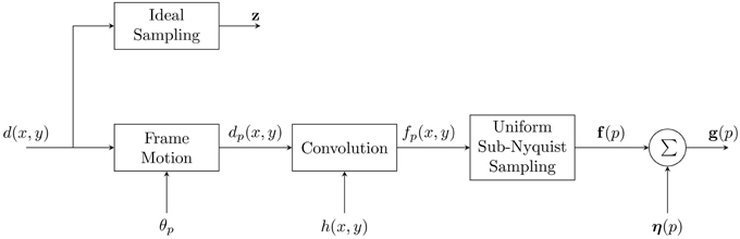
Figure 1. Forward observation model relating the desired continuous image, d(x, y) to the observed LR frames, g(p).

The final step in the block diagram is the noise block. We assume the noise is additive Gaussian noise with zero mean and variance of σ²_η. Thus, LR output frame p can be written in a lexicographical form as

$\begin{array}{cc}g(p)=f(p)+\eta (p),& (5)\end{array}$

where η(p) ~ N (0, σ²_η I). Note that for the model in Figure 1, the motion and convolution blocks can be commuted for translational motion [8]. The blocks can also be approximately commuted for affine motion under certain conditions [13]. After the commutation, the uniform sampling block can be replaced with a nonuniform sampling block that incorporates samples from all P LR frames on a common grid. This provides a nonuniformly sampled version of f(x, y), but with a denser sampling grid than a single frame provides. The noisy version of these nonuniform samples are represented here in lexicographical notation as g = [g₁, g₂, …, g_JP]^T.

3. Collaborative Adaptive Wiener Filter for Super-Resolution

3.1. CAWF Overview

The goal of the proposed CAWF SR is to estimate z from the observed LR frames, g(p), for p = 1, 2, …, P. In order to help the reader follow and easily understand the CAWF concept, we define some CAWF parameters in Table 1. The CAWF SR algorithm is shown in Figure 2. First, subpixel registration is done to place all of the observed LR samples on a common HR grid. The registration is done by using the gradient-based registration technique described in Hardie et al. [20], Irani and Peleg [21], Lucas and Kanade [22]. As mentioned in Section 2, the full set of samples are represented by the vector g. The CAWF SR method employs a W × W HR pixel spanning moving patch that passes over the HR grid in steps of L HR pixels in the horizontal and vertical dimensions. Let the observed samples that lie within the span of the i'th patch be denoted with the vector g_i. Let the number of pixels in each of these vectors be denoted as K. Note that K will be constant because we are considering only translational intra-frame motion, and we move patches only in LR pixel spacings across the HR grid. At each reference patch position, we identify the M most similar patches within a search window about the reference patch of size Z × Z HR pixels. In particular, for a given reference patch index i, we compute the following distances

$\begin{array}{cc}{D}_{i,j}=\frac{1}{\sqrt{2K}}\parallel g_i-g_j{\parallel }_2,& (6)\end{array}$

for j ∈ S_i, where S_i contains the window indices within the search window. We select the M patches corresponding to the M smallest distances. All pixels in the similar patches, including the reference patch, are concatenated in one vector. This combined vector is given by ${\tilde{g}}_i$ = [g^T_{si, 1}, g^T_{si, 2}, …, g_si,M^T]^T, where s_i = [s_{i, 1}, s_i,2, …s_i,M]^T. To illustrate this multi-patch selection process, Figure 3 shows an L = 3 HR grid made from three registered LR frames. The solid red box is the reference patch, and the blue boxes represent the identified similar patches. The large green box represents the span of the search window.

TABLE 1

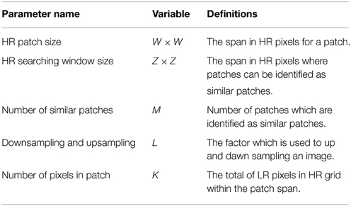
Table 1. CAWF parameters definitions.

FIGURE 2

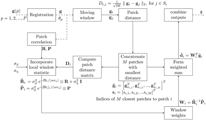
Figure 2. Block diagram illustrates the proposed CAWF SR algorithm. Dashed lines mean the process occurs one time for the entire process while continuous lines mean the process repeats for each moving window (J times).

FIGURE 3

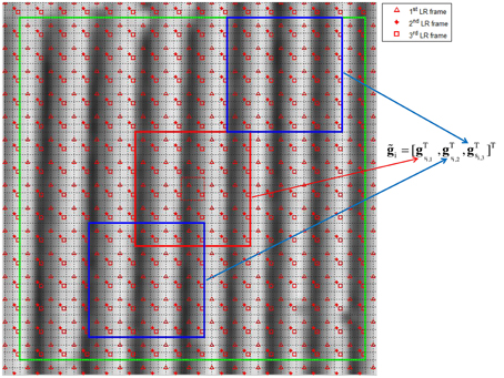
Figure 3. The HR grid shows the LR pixel locations for three frames (triangular, star, and square). The large green box represents the searching window span (45 × 45 HR pixels). The red box represents the reference patch while the blue ones represent its similar (each one is 15 × 15 HR pixels). The small dashed red box represents the estimation window (3 × 3 HR pixels)

The CAWF SR method estimates the L × L HR pixels in the center of each observation patch. This L × L estimation window is shown in Figure 3 as a small red dashed box. All of the pixels in the ${\tilde{g}}_i$ are used in a weighted to estimate these HR pixels. This is given by

$\begin{array}{cc}{\widehat{d}}_i=W_i^T{\tilde{g}}_i,& (7)\end{array}$

where $\widehat{d_i}$ = [d_i,1, d_i,2, …, d_i,L²]^T is a vector of estimated desired pixels, and Wi is a matrix of weights. After processing the entire image, all of these outputs are combined to form the estimated HR image, denoted as $\widehat{z}$. The weights are designed to minimize mean squared error (MSE) [17] and are given by

$\begin{array}{cc}{W}_i={\tilde{R}}_i{}^{-1}{\tilde{P}}_i,& (8)\end{array}$

where ${\tilde{R}}_i=E\left\{{\tilde{g}}_i{\tilde{g}}_i^T\right\}$ is a KM × KM auto-correlation matrix for the multi-patch observation vector ${\tilde{g}}_i$, and ${\tilde{P}}_i=E\left\{{\tilde{g}}_i{d}_i^T\right\}$ is a KM × L² cross-correlation matrix between the multi-patch observation vector, ${\tilde{g}}_i$, and the desired vector, d_i. Note that the vectors involved are treated as random vectors here, and E{·} represents the expectation operator. The correlations are modeled using a new nonuniform multi-patch correlation model described in Section 3.2.

3.2. Nonuniformly Sampled Multi-Patch Correlation Model

This section presents the nonunifomly sampled multi-patch correlation model used to provide the correlations needed for Equation (8). The model is similar to that in Mohamed and Hardie [17], but here applies to the nonunifomly sampled multi-patch observation vector ${\tilde{g}}_i$. In particular, the auto-correlation matrix model for ${\tilde{g}}_i$ is given by

$\begin{array}{cc}{\tilde{R}}_i={\sigma }_d^2 e^{-D_i/(\alpha {\sigma }_{\eta })}\otimes R+{\sigma }_{\eta }^2 I,& (9)\end{array}$

and the cross correlation matrix is given by

$\begin{array}{cc}{\tilde{P}}_i={\sigma }_d^2 e^{-{[D_i]}_1/(\alpha {\sigma }_{\eta })}\otimes P,& (10)\end{array}$

where I is a KM × KM identity matrix, ⊗ is a Kronecker product, σ²_d is the variance of desired image, α is the patch similarity decay, D_i is an M × M distance matrix between patches, and [D_i]₁ is the first column of the distance matrix. The terms R and P represent the auto-correlation and cross-correlation matrices for a single patch. More will be said about these shortly. In our model, these single patch statistics are “modulated” by the distance matrix to account for interpatch similarity. The parameter α is a tuning parameter to govern the strength of this modulation. The SNR is incorporated into the model with the selection of σ²_d and σ²_η. The distance matrix is populated using the distance metric in Equation (6) using the M similar patches as follows

$\begin{array}{cc}{D}_i=\left[\begin{array}{cccc}{D}_{s_{i,1},s_{i,1}}& D_{s_{i,1},s_{i,2}}& \cdots & D_{s_{i,1},s_{i,M}}\\ D_{s_{i,2},s_{i,1}}& D_{s_{i,2},s_{i,2}}& \cdots & D_{s_{i,2},s_{i,M}}\\ ⋮& ⋮& \ddots & ⋮\\ D_{s_{i,M},s_{i,1}}& D_{s_{i,M},s_{i,2}}& \cdots & D_{s_{i,M},s_{i,M}}\end{array}\right].& (11)\end{array}$

Let us now consider the single patch statistics. Note that

$\begin{array}{cc}R=E\left\{\overline{f}{\overline{f}}^T\right\},& (12)\end{array}$

is the K × K auto-correlation matrix of a single noise-free patch obtained from a variance-normalized desired image. The matrix

$\begin{array}{cc}P=E\left\{\overline{f}{\overline{d}}^T\right\},& (13)\end{array}$

is the K × L² cross-correlation matrix for a single noise-free patch obtained from a variance-normalized desired image and the desired pixels in the estimation window. The single patch statistics differ from those in Mohamed and Hardie [17] in that here a single patch is a nonuniformly sampled patch made up of samples from multiple registered LR frames. The relative positions of the samples in the patch depend on the particular interframe registration. Thus, we model these statistics based on continuous-space correlation functions in the same manner as that described in Hardie [8]. In particular, we assume the desired image is a wide sense stationary and we get auto-correlation of normalized noise-free image as

$\begin{array}{cc}{r}_{\overline{f}\overline{f}}(x,y)=r_{\overline{d}\overline{d}}(x,y)\ast h(x,y)\ast h(-x,-y),& (14)\end{array}$

where $r_{\overline{d}\overline{d}}$(x, y) is the autocorrelation function of the variance normalized desired image. Following the approach in Hardie [8], this is modeled as

$\begin{array}{cc}{r}_{\overline{d}\overline{d}}(x,y)={\rho }^{\sqrt{x^2+y^2}},& (15)\end{array}$

where ρ is auto-correlation decay constant. Similarly, the cross-correlation between noise-free signal obtained from a variance normalized desired image and the variance normalized desired image is given by

$\begin{array}{cc}{r}_{\overline{d}\overline{f}}(x,y)=r_{\overline{d}\overline{d}}(x,y)*h(x,y).& (16)\end{array}$

Since the motion is global translation, spacing between LR pixels is periodic (i.e., the same pattern) for the entire HR grid. With knowledge of the shifts between all LR frames, θ_p, horizontal and vertical distances between all samples in a patch can be computed easily. Then by applying these displacements to Equation (15) and then into Equations (16) and (14), we can fill both correlation matrices in Equations (12) and (13).

Finally, combining (8) with (12) and (13), we can express the CAWF SR weights as

$\begin{array}{cc}{W}_i={\tilde{R}}_i{}^{-1}{\tilde{P}}_i={\left[e^{-D_i/(\alpha {\sigma }_{\eta })}\otimes R+\frac{{\sigma }_{\eta }^2}{{\sigma }_d^2} I\right]}^{-1} e^{-{[D_i]}_1/(\alpha {\sigma }_{\eta })}\otimes P.& (17)\end{array}$

Note the weight matrix, W_i, is of size KM × L² where each column has the weights to estimate one particular HR pixel in the i'th estimation window. Before applying the weights, we follow the approach in Hardie [8] and normalize each column of weights to sum to one to avoid possibly creating a grid artifact if processing non-zero mean data. Using the model to compute the required correlations, note that there are two key tuning parameters. One is the auto-correlation decay, ρ, which controls the correlation between pixels within a given patch used to form R and P. The other parameter is the patch similarity decay, α, which controls the correlation between patches. The SNR also plays a role in shaping the correlations and ultimately the weights. Note that for a high SNR, the CAWF filter is more aggressive and relies less on spatial correlation for noise reduction. In low SNR imagery, the opposite is true. Also, note that when highly similar patches are found, as reflected in the distance matrix, the weights adapt to this and provide more aggressive SR processing. When no similar patches are found, the CAWF effectively reverts to the AWF method, primarily weighting only the reference patch. The relationship between the distance matrix and weights is explore more thoroughly for image restoration in Mohamed and Hardie [17].

4. Results and Discussion

In this section, the efficacy of the CAWF SR method is demonstrated. We compare against a single frame bicubic interpolation and the AWF SR method, in order to demonstrate the advantages of mutli-patch processing. Note that AWF SR is equivalent to CAWF SR when M = 1. We present results with both simulated data and real data. The real data represent raw data directly from the imaging sensor. In the case of the simulated data, we begin with a very high resolution and high signal-to-noise ratio image (not from the the sensor used for the real data). We then artificially degrade this ideal image with simulated motion, PSF blur (we follow the approach in Hardie [8] and modeled the diffraction from a circular exit pupil and spatial detector integration), downsampling, and noise, according to the model in Figure 1. The simulation is designed to mimic the real sensor to the greatest degree possible. That is, we simulate the same detector pitch, f-number, downsampling factor, and system PSF, as the real camera. All of the processing, simulation, and sensor parameters used in the are provided in Tables 2, 3. The simulated data allow for a quantitative performance analysis based on objective truth.

TABLE 2

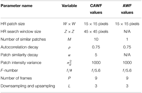
Table 2. The AWF and the CAWF system parameters which are used for both real and simulated data results.

TABLE 3

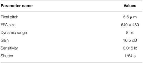
Table 3. Imaging Source camera (DMK 23U618) specifications.

The real camera data are acquired with an 8 bit gray-scale imaging source camera model DMK 23U618. Table 3 presents the camera specifications [23]. We assume a wavelength of λ = 0.55 μm and employ f/5.6 optics. Based on Equation (3), the Nyquist detector pitch would be δ_s = 1.54 μm. Thus, the camera, with its 5.6 μm detector pitch, is under-sampled by a factor of 3.64. Because of the optical transfer function, there tends to be relatively little energy near the SR folding frequency. Thus, in practice, we find that good results can be obtained with a slightly smaller upsampling factor of L = 3 and this is what we use for the presented results. For both the simulated data and real data, we use the same camera specifications to model the PSF and use L = 3 for downsampling and for SR upsampling.

With regard to performance metrics, we use a subjective visual assessment for the real data. For the simulated data, we use the peak signal-to-noise ratio (PSNR) metric, which is defined as

$\begin{array}{cc}PSNR\left(z,\widehat{z}\right)=10{\log }_{10}\left(\frac{{255}^2}{\frac{1}{N}{\displaystyle \sum _{i=1}^N{\left(z_i-{\widehat{z}}_i\right)}^2}}\right).& (18)\end{array}$

We also use the structure similarity index (SSIM), which is defined in Wang et al. [24].

4.1. Simulated Data

The first experiment in the simulated data results is a visual demonstration of the CAWF performance. We use the uncompressed 8 bit Kodak test image “Lighthouse” (Kodim19) [25] which we have converted to grayscale. We utilize the parameter values in Table 1 and follow the observation model in Figure 1 to get the LR frames. We blur the Lighthouse image with the prescribed PSF, shift it by random amounts, down samples these images by L = 3 and add Gaussian noise with σ_η = 10. We generate a total of P = 9 LR frames in this manner. Figure 4 shows the nine truth translational shifts as well as the estimated ones. The HR Lighthouse image is shown in Figure 5A and the first LR frame is shown in Figure 5B. The results for single frame bicubic interpolation, AWF SR and CAWF SR are shown for two regions of interest (ROIs) in Figures 6, 7. The first and second HR truth ROIs are shown in Figures 6A, 7A, respectively. The outputs of the bicubic interpolation for both ROIs are shown in Figures 6B, 7B. The effects of noise can be seen as “blotches” in the flat areas of the image. Aliasing and blurring are clearly evident along the fence. The AWF outputs are shown in Figures 6C, 7C, and the CAWF outputs are shown in Figures 6D, 7D. Examining the the outputs of AWF and CAWF, it is clear that both methods provide better resolution than bicubic interpolation. However, the CAWF method appears to provide better noise suppression. Quantitative results using seven Kodak test images are provided in Table 4. We use the same PSF as before with L = 3, P = 9, and σ_η = 10. Both PSNR and SSIM results are provided. Note that in average the CAWF PSNR is higher than the AWF PSNR by approximately 0.5 dB, and the SSIM is greater by approximately 0.04 (Bold numbers means the highest performance).

FIGURE 4

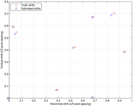
Figure 4. The translational truth and estimated shifts for the nine simulated LR frames.

FIGURE 5

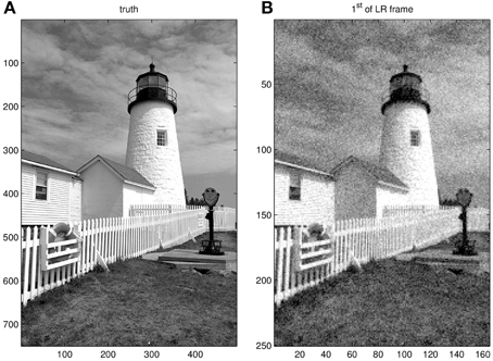
Figure 5. Lighthouse image. (A) Truth image and (B) first simulated LR frame with L = 3 and σ_η = 10.

FIGURE 6

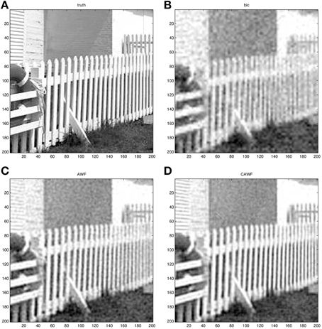
Figure 6. The first Lighthouse ROI. (A) The truth image, (B) bicubic output image, (C) AWF SR output image, and (D) the CAWF output image. Processing is done using L = 3, P = 9, and σ_η = 10.

FIGURE 7

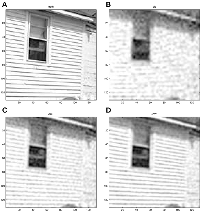
Figure 7. The second Lighthouse ROI. (A) The truth image, (B) bicubic output image, (C) AWF SR output image, and (D) the CAWF output image. Processing is done using L = 3, P = 9, and σ_η = 10.

TABLE 4

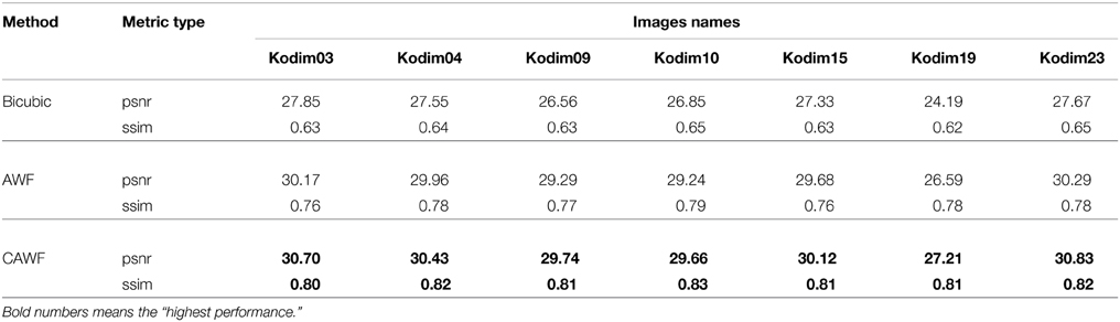
Table 4. Quantitative performance of the bicubic, the AWF and the CAWF outputs for 7 Kodak images for L = 3, P = 9, and σ_η = 10.

The next experiment shows that the improvement in perfromance seen with CAWF is observed even with many noise and shift realizations. In partcular, we use the lighthouse image and simulate 50 sets of LR frames. Each set is obtained with different realization of random intra-frame shifts and noise samples. The results are shown in Figure 8, with PSNR shown in Figure 8A, and SSIM shown in Figure 8B. From Figure 8A, the means of PSNR are 27.15, 26.55, and 24.20 for CAWF, AWF, and single frame bicubic interpolation, respectively. The standard deviations of PSNR for the same methods are 0.0602, 0.0550, and 0.0102. Also, the means of SSIM shown in Figure 8B are 0.81, 0.78, and 0.62 for CAWF, AWF, and single frame bicubic interpolation, respectively. The respective standard deviations of SSIM are 0.0021, 0.0012, and 0.0015.

FIGURE 8

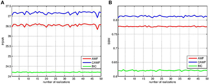
Figure 8. PSNR and SSIM statistics for the various SR algorithms over 50 shift and Gaussian noise patterns realizations (A) PSNR and (B) SSIM. These results are obtained for Lighthouse image when L = 3, P = 9 and σ_η = 10.

Results are shown in Figure 9 that illustrate the impact of changing the number of similar patches, M, in the CAWF SR method using the lighthouse image (Kodim19). The PSNR and SSIM of the CAWF SR outputs are shown in Figures 9A,B, respectively. For these results, we again use the parameters listed in Table 2, but vary M from 1 to 17. Note that M = 1 means no patch similarity is utilized, and the CAWF method reduces to the AWF. Note that PSNR increase significantly with M for M ≤ 10, and there appears to be a “knee” in the curve near M = 10. It is for this reason that we have elected to use M = 10 in the previous results. A similar patterns is seen with SSIM in Figure 9B.

FIGURE 9

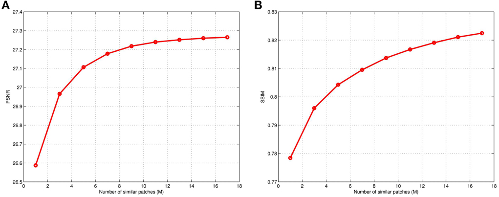
Figure 9. Results showing CAWF SR performance as a function of the number of similar patches M (A) PSNR and (B) SSIM. These results are obtained with L = 3, P = 9, σ_η = 10 and M varying from 1 to 17.

In a final simulated data experiment, we study the impact of noise level and the number of LR input frames used on the AWF and CAWF SR methods. These results are presented in Figures 10, 11. The lighthouse image is used with the parameters in Table 2, but with P ranging from 1 to 9. The PSNR results for σ²_η = 1, 25, 100 and 225 are shown in Figures 9A–D, respectively. A similar set of results, but with the SSIM metric, are shown in Figure 11. Clearly, increasing the number of input frame improves performance for both CAWF and AWF. Also, the relative improvement increases with noise level. This trend is shown in Figure 12. Note that CAWF SR consistently outperforms AWF SR in these results. Table 5 shows quantitative results for the bicubic, AWF and CAWF for the four levels of noise when P = 9. We conclude these results from Figures 10, Figure 11.

FIGURE 10

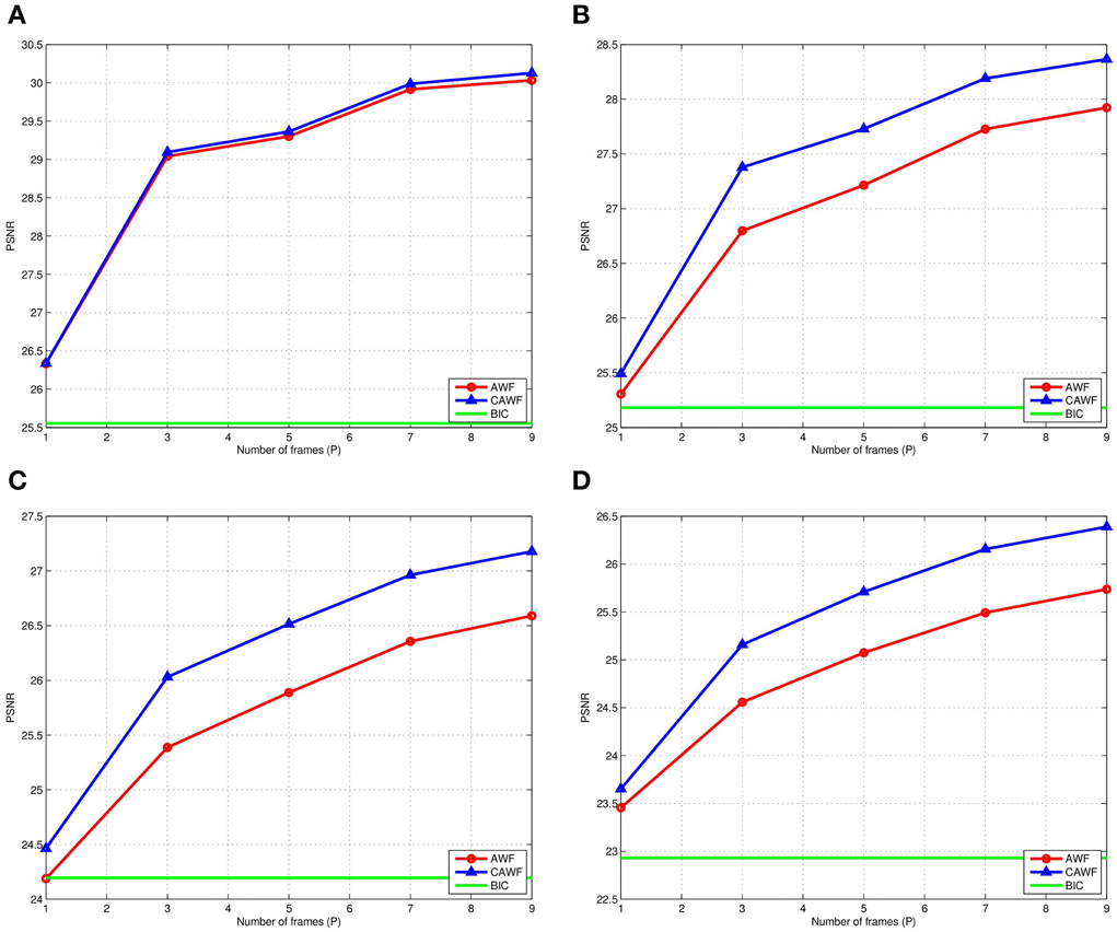
Figure 10. The PSNR for AWF, CAWF, and the bicubic outputs with different levels of noise. (A) σ_η = 1, (B) σ_η = 5, (C) σ_η = 10, and (D) σ_η = 15. These results are obtained with M = 10 and the number of frames, P, varies from 1 to 9.

FIGURE 11

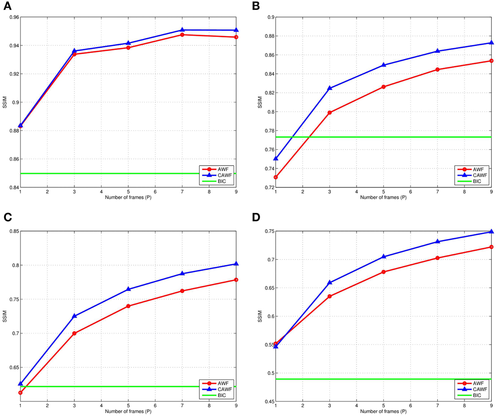
Figure 11. The SSIM for AWF, CAWF, and the bicubic outputs with different levels of noise. (A) σ_η = 1, (B) σ_η = 5, (C) σ_η = 10, and (D) σ_η = 15. These results are obtained with M = 10 and the number of frames, P, varies from 1 to 9.

FIGURE 12

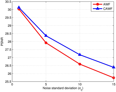
Figure 12. The PSNR for AWF and CAWF, with different levels of noise. These results are obtained with M = 10 and the number of frames, P = 9.

TABLE 5

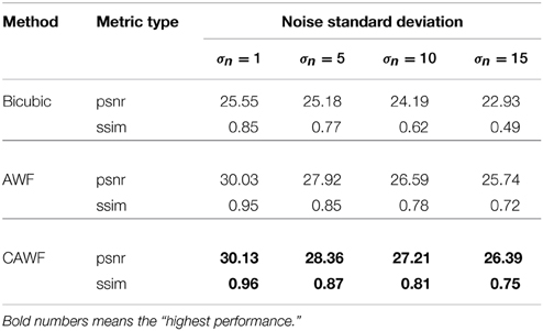
Table 5. Quantitative performance of the bicubic, the AWF and the CAWF outputs for the Lighthouse image when L = 3, P = 9 and four levels of noise.

4.2. Real Data

In this section, two sets of real data are processed and presented. In both data sets, we get the LR frames by panning the camera described in Table 3 across a scene. We utilize nine frames as inputs (P = 9). We employ the parameters listed in Table 2 for processing. Also we assume the noise is additive zero-mean Gaussian noise with variance of σ²_η. Using the sample variance in a flat region of the scene, we estimate the noise standard deviation for both data sets to be σ_η = 5.

The estimated intra-frame translational shifts for the first data set are shown in Figure 13. The first full (320 × 320) LR frame from this dataset is shown in Figure 14. Aliasing can be seen in this imagery, especially in the chirp pattern shown in the left lower corner. To better illustrate the SR results, two ROIs are selected. These processed ROIs are shown in Figure 15. The bicubic results are shown in Figures 15A,B. The AWF results are shown in Figures 15C,D. Finally, the CAWF results are shown in Figures 15E,F. As with the simulated data, the AWF and CAWF methods appear far better than the bicubic interpolation in terms of aliasing reduction and resolution enhancement. However, the CAWF outputs appear to show more detail than the AWF outputs do. This can be seen in the high frequency regions of the chirp ROI and the parallel lines above and below the word “signal.”

FIGURE 13

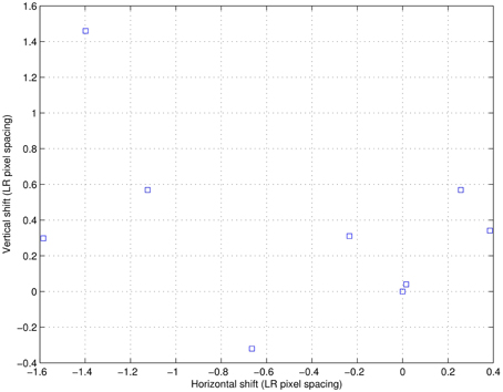
Figure 13. The estimated shifts for the nine real LR frames (data set I).

FIGURE 14

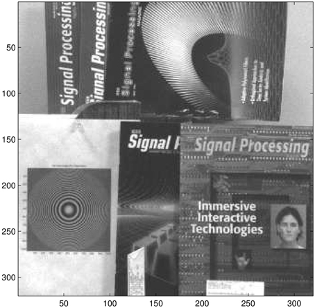
Figure 14. The first LR frame (data set I) which has been captured by an 8 bit gray-scale Imaging Source camera (DMK 23U618) in our University of Dayton Image Processing Laboratory.

FIGURE 15

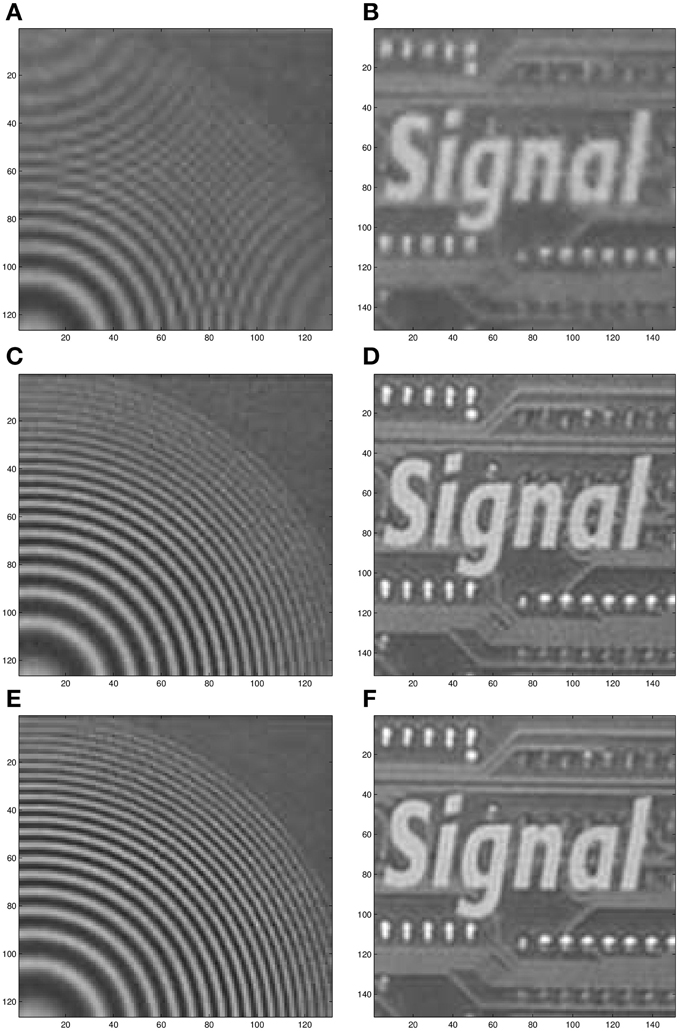
Figure 15. Two processed ROIs from the real image sequence (data set I). Bicubic output for ROI 1 (A) and ROI 2 (B). AWF SR output for ROI 1 (C) and ROI 2 (D). CAWF SR output for ROI 1 (E) and ROI 2 (F).

For the second real data set, the estimated intra-frame translational shifts are shown in Figure 16. Figure 17 shows the first full (300 × 300) LR frame from this second dataset. Also two ROIs are chosen, one shows a portion of the notebook in the scene, and the other is part of the window mullion. These processed ROIs are shown in Figure 18. The bicubic results are shown in Figures 18A,B. The AWF results are shown in Figures 18C,D. Finally, the CAWF results are shown in Figures 18E,F. We believe that the performance of CAWF SR method using the real data is consistent with that obtained with the simulated data, and that CAWF SR does offer a notable improvement over AWF SR.

FIGURE 16

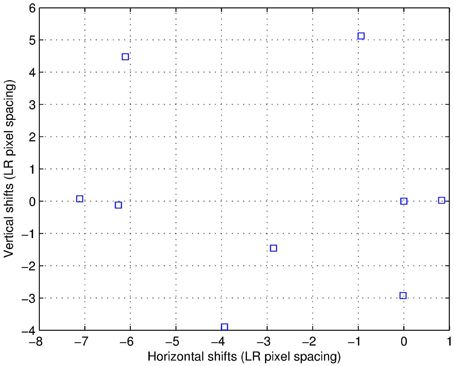
Figure 16. The estimated shifts for the nine real LR frames (data set II).

FIGURE 17

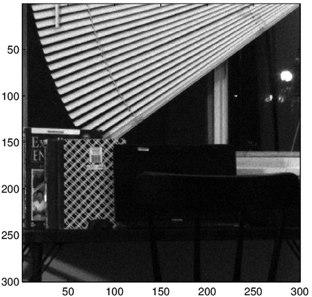
Figure 17. The first real LR frame (data set II) which has been captured by an 8 bit gray-scale Imaging Source camera (DMK 23U618).

FIGURE 18

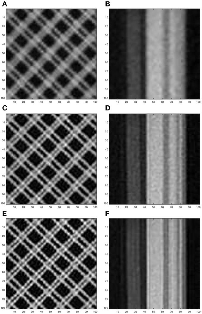
Figure 18. Two processed ROIs from the real image sequence (data set II). Bicubic output for ROI 1 (A) and ROI 2 (B). AWF SR output for ROI 1 (C) and ROI 2 (D). CAWF SR output for ROI 1 (E) and ROI 2 (F).

5. Conclusion

We have proposed a novel CAWF method for multi-frame SR. The first step of the CAWF SR method is to register all LR frames one a common HR grid. Then, for each LR pixel position on the HR grid, we identify the M most similar patches within a given search window about the reference patch. A single-stage weighted sum of the pixels in the similar patches is used to estimate the L × L HR pixels in estimate window at the reference patch. The weights are based on a new nonuniformly sampled multi-patch correlation model. The CAWF SR method can be viewed as an extension of AWF SR [8] using mutli-patch processing. Using multiple similar patches to form the estimate allows the CAWF technique to exploit self-similarity to greatly increase the noise robustness over the AWF SR method. In light of the CAWF method, The AWF method can be viewed as a special case where M = 1 and only the reference patch is included in the weighted sum to form the estimate. Like the AWF SR, CAWF SR can perform nonuniform interpolation, deblurring, and denoising jointly. The big advantage of the CAWF, vs. the AWF, is improved performance in low SNR data. From the real and the simulated image data, the CAWF SR outperforms AWF SR for all scenarios and cases tested. Although the most benefit is seen when the noise level is high. We believe the CAWF SR approach might be beneficial in several other applications as well, including those where the AWF is successful [9–13].

Author Contributions

KM coded the CAWF SR algorithm, collected all of the data used here, and prepared all of the experimental results. RH suggested the CAWF SR approach as an extension of the AWF SR method. Both KM and RH contributed to the writing and editing of the current manuscript.

Conflict of Interest Statement

The authors declare that the research was conducted in the absence of any commercial or financial relationships that could be construed as a potential conflict of interest.

References

1. Hou HS, Andrews H. Cubic splines for image interpolation and digital filtering. IEEE Trans Acoust Speech Signal Process. (1978) 26:508–17. doi: 10.1109/TASSP.1978.1163154

CrossRef Full Text | Google Scholar

2. Nasir H, Stankovi V, Marshall S. Singular value decomposition based fusion for super-resolution image reconstruction. Signal Process. (2012) 27:180–91. doi: 10.1016/j.image.2011.12.002

CrossRef Full Text | Google Scholar

3. Szydzik T, Callico GM, Nunez A. Efficient FPGA implementation of a high-quality super-resolution algorithm with real-time performance. IEEE Trans Consum Electron. (2011) 57:664–72. doi: 10.1109/TCE.2011.5955206

CrossRef Full Text | Google Scholar

4. Song BC, Jeong SC, Choi Y. Video super-resolution algorithm using bi-directional overlapped block motion compensation and on-the-fly dictionary training. IEEE Trans Circuits Syst Video Technol. (2011) 21:274–85. doi: 10.1109/TCSVT.2010.2087454

CrossRef Full Text | Google Scholar

5. Mancas-Thillou C, Mirmehdi M. An introduction to super-resolution text. In: Chaudhuri B, editor. Digital Document Processing. Advances in Pattern Recognition. London: Springer (2007). p. 305–27.

Google Scholar

6. Lin F, Fookes C, Chandran V, Sridharan S. Super-resolved faces for improved face recognition from surveillance video. In: Lee SW, Li S, editors. Advances in Biometrics. Vol. 4642, of Lecture Notes in Computer Science. Berlin; Heidelberg: Springer (2007). p. 1–10.

Google Scholar

7. Barner KE, Sarhan AM, Hardie RC. Partition-based weighted sum filters for image restoration. IEEE Trans Image Process. (1999) 8:740–5. doi: 10.1109/83.760341

PubMed Abstract | Full Text | CrossRef Full Text | Google Scholar

8. Hardie R. A fast image super-resolution algorithm using an adaptive wiener filter. IEEE Trans Image Process. (2007) 16:2953–64. doi: 10.1109/TIP.2007.909416

PubMed Abstract | Full Text | CrossRef Full Text | Google Scholar

9. Hardie RC, LeMaster DA, Ratliff BM. Super-resolution for imagery from integrated microgrid polarimeters. Opt Express. (2011) 19:12937–60. doi: 10.1364/OE.19.012937

PubMed Abstract | Full Text | CrossRef Full Text | Google Scholar

10. Narayanan BN, Hardie RC, and Balster EJ. Multiframe adaptive Wiener filter super-resolution with JPEG2000-compressed images. EURASIP J Adv Signal Process. (2014) 2014:55. doi: 10.1186/1687-6180-2014-55

CrossRef Full Text | Google Scholar

11. Karch BK, Hardie RC. Adaptive Wiener filter super-resolution of color filter array images. Opt Express. (2013) 21:18820–41. doi: 10.1364/OE.21.018820

PubMed Abstract | Full Text | CrossRef Full Text | Google Scholar

12. Hardie RC, Barnard KJ. Fast super-resolution using an adaptive Wiener filter with robustness to local motion. Opt Express. (2012) 20:21053–73. doi: 10.1364/OE.20.021053

PubMed Abstract | Full Text | CrossRef Full Text | Google Scholar

13. Hardie RC, Barnard KJ, Ordonez R. Fast super-resolution with affine motion using an adaptive wiener filter and its application to airborne imaging. Opt Express. (2011) 19:26208–31. doi: 10.1364/OE.19.026208

PubMed Abstract | Full Text | CrossRef Full Text | Google Scholar

14. Milanfar P. Super-Resolution imaging. In: Digital Imaging and Computer Vision. CRC Press (2011). Available online at: http://books.google.com/books?id=fjTUbMnvOkgC

15. Danielyan A, Foi A, Katkovnik V, Egiazarian K. Image and video super-resolution via spatially adaptive blockmatching filtering. In: Proceeding of International Workshop on Local and Non-local Approximation in Image Processing (LNLA). Lausanne (2008).

Google Scholar

16. Dabov K, Foi A, Egiazarian K. Video denoising by sparse 3D transform-domain collaborative filtering. In: 15th European Signal Processing Conference (EUSIPCO). Poland: Poznan (2007).

Google Scholar

17. Mohamed K, Hardie R. A collaborative adaptive Wiener filter for image restoration using a spatial-domain multi-patch correlation model. EURASIP J Adv Signal Process. (2015) 2015:6. doi: 10.1186/s13634-014-0189-3

CrossRef Full Text | Google Scholar

18. Hardie RC, Barnard KJ, Bognar JG, Armstrong EE, Watson EA. High-resolution image reconstruction from a sequence of rotated and translated frames and its application to an infrared imaging system. Opt Eng. (1998) 37:247–60. doi: 10.1117/1.601623

CrossRef Full Text | Google Scholar

19. Fiete RD. Image quality and FN/p for remote sensing systems. Opt Eng. (1999) 38:1229–40. doi: 10.1117/1.602169

CrossRef Full Text | Google Scholar

20. Hardie R, Barnard K, Bognar J, Armstrong E, Watson E. High-resolution image reconstruction from a sequence of rotated and translated frames and its application to an infrared imaging system. Opt Eng. (1998) 37:247–60. doi: 10.1117/1.601623

CrossRef Full Text | Google Scholar

21. Irani M, Peleg S. Improving Resolution by Image Registration. CVGIP Graph Models Image Process. (1991) 53:231–9. doi: 10.1016/1049-9652(91)90045-L

CrossRef Full Text | Google Scholar

22. Lucas BD, Kanade T. An iterative image registration technique with an application to stereo vision. In: Proceedings of the 7th International Joint Conference on Artificial Intelligence - Vol. 2, IJCAI'81. San Francisco, CA: Morgan Kaufmann Publishers Inc. (1981). p. 674–9.

Google Scholar

23. Sony. The Imaging Source Technology Based on Standards (2014). Available online at: http://www.theimagingsource.com/en_US/products/cameras/usb-cmos-ccd-mono/dmk23u618/

24. Wang Z, Bovik AC, Sheikh HR, Simoncelli EP. Image quality assessment: from error visibility to structural similarity. IEEE Trans Image Process. (2004) 13:600–12. doi: 10.1109/TIP.2003.819861

PubMed Abstract | Full Text | CrossRef Full Text

25. Kodak. Kodak Lossless True Color Image Suite (1999). Available online at: http://r0k.us/graphics/kodak/. [Online: Accessed 15-Nov-1999].