Compaction of granular material inside confined geometries

1. Introduction

When granular materials are placed in confined geometries, we often observe a significant portion of the stress being redirected toward the confining boundaries. This phenomenon has been systematically studied for many systems [1–3], most notably in silos, beginning with Janssen [4]. Force redirection has been attributed to the granular nature of the material, and has in many cases been shown to be well represented by a constant coefficient, known as the Janssen coefficient K, defined in one spatial dimension as

$K={\sigma }_r/{\sigma }_n,$

where σ_r is the redirected stress due to some applied normal stress σ_n. Here we investigate the development of stresses within a granular packing, confined vertically between two horizontal plates, with no walls in the remaining directions, subjected to a rigid piston impacting it from one side. As the piston moves, granular material is compacted near the piston, and with increasing displacement of the piston, the size of the packing increases. Such an accumulation process is known to occur in the petroleum industry, where sand is liberated from the host rock during extraction, altering the underground morphology of cracks [5, 6]. This may also be relevant for understanding proppant flowback in propped fractures [7]. Additionally, this geometry is representative of a number of recent experimental studies in Hele-Shaw cells [8–11] where the validity of Janssen stress redirection has not been ascertained.

There are a number of interesting patterns which form when a granular material is displaced by a flexible interface in such a geometry [9, 11]. The nature of the patterns have been shown to depend on many factors, primarily the initial packing fraction and the rate of displacement [10]. For this reason, we here investigate the microstructural and mechanical evolution of such a system under these conditions. To reduce the complexity of the system, we consider only a rigid piston.

We are interested in systems which are highly confined. In common experiments with granular material inside Hele-Shaw cells, there are in general fewer than 20 grain diameters between the two Hele-Shaw plates, typically down to around 5 grain diameters [10]. As the confinement increases, i.e., as the gap spacing decreases, we expect a transition from three dimensional behavior toward a behavior governed by the boundaries, as demonstrated for vertical silos in Bratberg et al. [12]. It is then of interest to study the changes that result from increasing confinement. We expect that altering the confinement will affect the force redistribution. A transition may occur for extremely confined systems where such an assumption concerning force redirection may not be valid.

Existing analytic models for the micromechanics of such a system generally reduce the problem to one spatial dimension (x), assuming that variations in both remaining directions (y and z) are small, although recently curved interfaces have also been described [8]. For simplicity, we consider a flat interface, and validate the analytic description with a discrete element model.

Firstly, in Section 2 describe the numerical model that has been used to simulate this system. In Section 3, we establish continuum properties which correspond to the analytic formulation, and show comparisons between the two. In particular, the limitations of current analytic models are identified. Finally, a parameter set is proposed that best fits the analytic theories for a wide range of system variables.

2. Materials and Methods

This paper is an investigation into the micromechanics of a system which is highly constrained by external boundaries. For this reason, it is ideal to use a particle based method to model the behavior, as the total number of grains in the system is small. Toward this end, we use a conventional soft sphere discrete particle approach, implemented in the open source code MercuryDPM (www.mercurydpm.org) [13, 14]. The geometry considered here, shown in Figure 1, consists of a rigid piston, oriented in a space r = {x, y, z}, with normal along the x axis, which pushes particles between two rigid plates, separated by a spacing D and having normals in the ±z directions, with two periodic boundaries in the remaining perpendicular direction, y. The coordinate system moves with the piston, such that it is located at x = 0 at all times. As the piston moves horizontally at a velocity u toward the grains, its displacement at any time t is then s = ut.

FIGURE 1

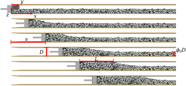
Figure 1. Particle positions during a single test, shown at six piston displacements s. Top to bottom: s = 0, 10, 20, 30, 40, and 50. Labels refer to the coordinate system x, y, and z, the gap height D, the plug length L and the initial packing fraction ϕ₀. Particles are colored by size, darker colors representing smaller particles.

We work in a system of non-dimensionalized units with the following properties; length and mass have been non-dimensionalized by the length d′_m and mass m′_m of the largest particle in the system, respectively, where the prime indicates that the quantity has dimension. The particle diameters, d, we use are therefore d ≤ 1, with material density defined by 4π(1/2)³ρ_p/3 = 1, or ρ_p = 6/π. Time is non-dimensionalized by the time taken for the largest particle to fall from rest its own radius under the action of gravity, so that a unit time is $t=\sqrt{d_m/g}$, which requires that g = 1. Other values are non-dimensionalized by a combination of these three scales, for example stress is non-dimensionalized by m′_mg′/d′²_m.

Particles are filled into the available space by assigning them to positions on a regular hexagonally close packed lattice, dimensioned such that particles of diameter 1 would be in contact. In all cases we use particles distributed uniformly in the range 0.5 ≤ d ≤ 1 to avoid crystallization, and to mimic the size range used in Sandnes et al. [10]. Variable particle filling is facilitated by changing the number of layers of the grid, such that the initial packing fraction, ϕ₀ defined in Equation (3), is approximately constant throughout the cell. From t = −10 to t = 0, gravity in the −z direction is increased from g = 0 to g = 1 to settle the grains in a loose packing. From t = 0 the piston begins to move at velocity u.

As shown in Figure 2, the particles' material properties are described by normal, tangential and rolling damped spring sliders [13, 15] with the properties contained in Table 1. These values have previously been calibrated to mimic 20 micron silica beads [16]. Here we neglect the role of adhesion between particles, which will become increasingly important as the physical size of the particles reduces. The walls are implemented such that they are rough; when a particle contacts a wall, the piston, or both, it is prohibited from rotating, i.e., μ_r = 1. Otherwise, the interaction properties are the same as between two particles, except that the walls and piston are of infinite mass. We therefore have a well defined macroscopic sliding friction of μ = 0.4 that does not depend on the rate of loading.

FIGURE 2

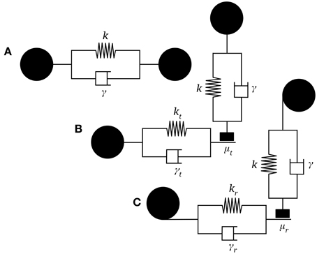
Figure 2. Contact laws used in the discrete element model. Interactions are characterized by (A) normal, (B) tangential and (C) rolling laws, parameterized by stiffnesses k, k_t and k_r, viscous dissipation γ, γ_t and γ_r and friction coefficients μ_t and μ_r. Full details are given in Luding [15].

TABLE 1

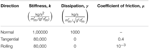
Table 1. Material properties of the spheres.

In the following Section we will firstly detail the important macroscopic quantities measured from a single simulation. We will then investigate the effect of three controlling parameters on the evolution of the system: the Hele-Shaw spacing D, the initial packing fraction ϕ₀ and the velocity of the piston, u. The piston rate, however, is not a priori a governing quantity, so we choose to control the piston rate via the inertial number, I, which is defined as $I=\dot{\gamma }{d}_m/\sqrt{P/{\rho }_p}$, which is the ratio of inertial to imposed stresses, where P is a typical pressure and $\dot{\gamma }$ is a typical shear strain rate [17]. Taking $\dot{\gamma }$ = u/D, and P = ρ_pgD, gives

$I=\frac{u{d}_m}{D^{3/2}{g}^{1/2}}=u{D}^{-3/2}.$

3. Results

As depicted in Figure 1, three distinct regions exist inside the system. These are termed the plug zone, where particles are densely packed near to the piston (x ≤ L), the undisturbed zone, far from the plug, and the transition zone, where the plug is accumulating. To define these regions systematically, we must first measure the solid fraction, ν = V_s/V_t, which is a local measure of the ratio of the volume of solids to the total volume. The solid fraction is coarse grained in one spatial dimension, x, as

$\begin{array}{cc}\nu (x,t)=\frac{1}{WD}{\displaystyle \sum _{i=1}^N{V}_i}\mathcal{W}(x-x_i(t)),& (1)\end{array}$

where N is the number of grains in the system, W is the width of the system, V_i is the volume of the i-th grain, x_i its center of mass and is the coarse graining function, chosen in this case to be a 1D normalized Gaussian function [14, 18]. Such a coarse graining method allows the coarse graining width to be defined, so that either the macro- or micro-structure is visible. We choose to use a coarse graining width equal to the maximum particle diameter, such that small scale variations are minimized, and smooth continuum fields are obtained [19]. All other continuum quantities are defined using the same coarse graining technique, presented in Goldhirsch [18], Weinhart et al. [14]. Using the definition (1), we denote the maximum solid fraction, ν_m, as an average over the solid fraction close to the wall at some time when the transition zone is far from the piston as

$\begin{array}{cc}{\nu }_m=\frac{1}{5D}{\displaystyle {\int }_{5D}^{10D}\nu }(x) dx,& (2)\end{array}$

where in practice a numerical integration is done over the discrete coarse grained cells, and the limits of 5D and 10D are chosen arbitrarily. We define the normalized packing fraction, ϕ(x, t), as ϕ = ν/ν_m, and note that in the absence of volumetric expansion or dilation of the granular material, ϕ is directly proportional to the height of the packing between the Hele-Shaw walls. The undisturbed zone is that which is maintained at the initial packing fraction ϕ₀, which is defined at time t = 0 as

${\varphi }_0=\frac{1}{5D}{\displaystyle {\int }_{5D}^{10D}\varphi }(x,t=0) dx.$

To delineate the plug, transition and undisturbed zones, at each time t we use linear regression to find the best linear fit to the points in the range ϕ = ϕ₀ + 0.1 to ϕ = 0.9, such that ϕD ≈ b − x tan θ, for some value of b and slope angle θ. Five examples of this are shown in Figure 3A. Using this best fit, we can define the point at which the plug zone meets the transition zone as the intersection of the best fit regression line and ϕ = 1, such that L = (b − D)/tan θ, as shown in Figure 3A. The value of L grows monotonically with piston displacement, as shown in Figure 3B. Conservation of mass implies that on average, if there is no volumetric change in the packing, and no slip between the grains and the walls, this relationship can be expressed as

$\begin{array}{cc}\frac{L}{s}=\frac{{\varphi }_0}{1-{\varphi }_0},& (3)\end{array}$

which is shown as the dashed line in Figure 3B. For all cases reported here, the value of θ does not appear to vary with increasing plug length L. The point at which the undisturbed zone meets the transition zone can then be defined in a similar manner as above, by the intersection of the best fit regression line with ϕ = ϕ₀. The coordination number, Z, (average number of contacts per particle), is fairly constant in the plug zone, (Figure 3C), increasing with compaction, as rearrangement occurs. Additionally, at large values of L the stresses are high enough to cause significant overlap of the particles (up to 1%). In the transition zone, significant particle rearrangement lowers the coordination number.

FIGURE 3

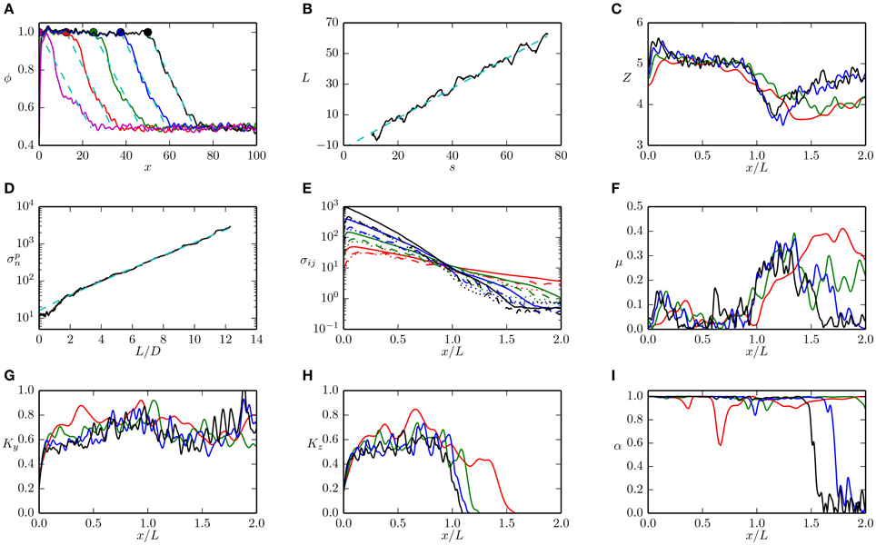
Figure 3. Evolution of coarse grained properties of the system with increasing piston displacement, s, for D = 5, ϕ₀ = 0.5 and I = 0.01. (A) Five examples of the normalized packing fraction of the particles, ϕ. The magenta, red, green, blue, and black lines indicate displacements which correspond to L = 0, 12.5, 25, 37.5, and 50 respectively. The same color scheme is used for each subsequent plot in this Figure unless stated otherwise. A filled circle indicates the measured value of L, and the cyan dashed line indicates the linear best fit measurement of the transition zone. (B) Evolution of the measured value of L with increasing displacement s drawn in black. The cyan line indicates the best linear fit to these points. (C) The coordination number, Z, as a function of normalized distance from the piston head, x/L. (D) Normal stress measured at the piston is shown in black. The cyan dashed line indicates the best fit estimate of Equation (6). (E) Normal stress distributions within the packing. Solid lines indicate σ_xx, dashed σ_yy and dotted σ_zz. (F) Apparent friction coefficient measured within the packing, μ = |σ_xz|/σ_zz. (G) Out of plane Janssen coefficient measured within the packing, K_y = σ_yy/σ_xx. (H) In plane vertical Janssen coefficient measured within the packing, K_z = (σ_zz − ρ_pνgD/2)/σ_xx. (I) Absolute value of the x component of the eigenvector of the major principal stress.

Coarse graining techniques in general cause measured fields to converge toward zero near boundaries [14]. While it is feasible to reconstruct these fields in general near individual boundaries, near the piston we have three distinct boundaries which all interact. To access stresses in this region, it is then preferable to directly measure the forces applied to the rigid boundaries of the system. Toward this end, we denote σ^p_n as the normal stress measured at the piston. This is shown as a function of piston displacement in Figure 3D. The stresses measured from coarse graining within the packing are shown in Figure 3E. In both cases, the stresses grow exponentially both with increasing L and decreasing x, as shown by the linearity in a semilog space in Figures 3D,E.

An analytic expression to describe this stress evolution was first derived in Knudsen et al. [9], assuming that: (a) the stress redirection in the z direction is described by a constant K_z = σ′_zz/σ_xx, where σ′_zz = σ_zz − Dρ_pν_mg/2 is the component of the vertical stress not due to gravity and (b) friction at the side walls is μ = σ_xy/σ_zz. It can be shown using force balance in the x direction that under these conditions, if there is no net acceleration,

$\frac{d{\sigma }_{xx}}{dx}=-\frac{2\mu K_z}{D}{\sigma }_{xx}-\mu {\rho }_p{\nu }_{m}g.$

By further assuming that the stress at x = L is a constant, i.e., σ_T ≡ σ_xx(x = L),

$\begin{array}{cc}{\sigma }_{xx}=\left({\sigma }_T+\frac{D{\rho }_p{\nu }_{m}g}{2K_z}\right)e^{2\mu K_z(L-x)/D}-\frac{D{\rho }_p{\nu }_{m}g}{2K_z}.& (4)\end{array}$

Previously, the threshold stress σ_T has been modeled as either estimated from experimental data [8], or as a constant by assuming sliding of a wedge of material [9, 11]. Here, we choose to model the threshold stress σ_T as a ϕ₀ dependent quantity by considering limit equilibrium of a wedge of material being displaced into the undisturbed zone, as shown in Figure 4. We assume a noncohesive Coulomb failure of the material internally, along a failure plane parallel to and meeting the surface of the transition zone. We additionally assume that the internal friction angle is also defined by μ. Limit equilibrium in the x direction can then be expressed using the notation defined in Figure 4 as F_x = T_b + T_icosθ, where F_x = Dσ_T, T_b = μW₀ = μD²ρ_pν_mg/(2 tan θ) and T_i = μW₁ cos θ = μD²ρ_pν_mgϕ²₀ cos θ/(2 tan θ) per unit length in the y direction. After some rearrangement this implies that

$\begin{array}{cc}{\sigma }_T=\frac{\mu D{\rho }_p{\nu }_{m}g}{2\tan \theta }(1+{\varphi }_0^2{\cos }^2\theta ).& (5)\end{array}$

FIGURE 4

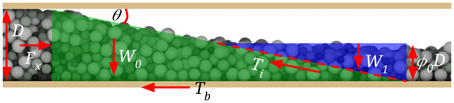
Figure 4. Limit equilibrium of the transition zone. For the pile to be displaced by a force F_x, two forces must be overcome; T_b, the basal traction due to the weight W₀ of the green region, and the x component of the internal sliding traction T_i along the assumed failure surface denoted by the dashed line, due to the normal component of the weight above the failure surface, W₁, of the blue region.

This assumption of the failure surface introduces no new parameters into the model, and as will be shown in the following, closely predicts the measured value of σ_T for a large range of system parameters. In the limit where ϕ₀ → 0, this definition reduces to that used in Knudsen et al. [9] and Sandnes et al. [11]. Including this new definition of the threshold stress, Equation (5), in Equation (4) gives

$\begin{array}{cc}{\sigma }_{xx}=\frac{D{\rho }_p{\nu }_{m}g}{2K_z}\left(\left(\frac{\mu K_z}{\tan \theta }(1+{\varphi }_0^2{\cos }^2\theta )+1\right)e^{2\mu K_z(L-x)/D}-1\right).& (6)\end{array}$

A best fit estimate is used to find K_z from Equation (6), and is shown as the dashed line in Figure 3D at x = 0, using the measured values of ν_m, θ and ϕ₀, which adequately captures the behavior of the system past L/D = 2. Before this limit, stress redistribution has not saturated, and σ_xx is less than the predicted value. We find the same transition value of L/D ≈ 2 for all cases reported here.

The measured value of apparent friction μ = σ_xz/σ_zz inside the packing, shown in Figure 3F shows that the system is far from failure inside the plug zone, and increasingly unstable in the transition zone. The out of plane Janssen coefficient, K_y = σ_yy/σ_xx, shown in Figure 3G, has large variations in x, but is not significantly affected by the formation of the plug. The in plane Janssen coefficient (Figure 3H), K_z = σ′_zz/σ_xx, however, is strongly influenced by the formation of the plug, and is relatively constant with increasing L inside the plug zone.

An underlying assumption of the Janssen stress redistribution is that when averaging over the width of the system (here in the y and z directions), the principal stress directions are parallel to the system geometry [4]. For this reason we measure α, the absolute value of the x component of the eigenvector of the major principal stress, which is shown in Figure 3I. When α ≈ 1 the major principal stress points along the x-axis, and when α ≈ 0, the principal stress lies in the yz plane. For x ≤ L we find that the major principal stress is collinear with the system geometry, and the Janssen stress model fits well. In a traditional silo problem, gravity acts parallel to the applied stress, and averaging across the width of a silo ensures the validity of this assumption. For this case, however, because the direction of gravity has broken the inherent symmetry of the silo problem, its validity is not ensured [20]. We do, however, find that this assumption holds well for this and all simulations reported here.

3.1. Gap Spacing

As motivated in Equation (6), the gap spacing D largely controls the magnitude of the stresses within the system. For this reason, we here vary this spacing systematically from D = 1 to D = 15, while maintaining ϕ₀ = 0.5 ± 0.05 and I = 0.01 (except for the case of D = 1, where ϕ₀ ≈ 0.66), as depicted for four values of D in Figure 5. To make a reasonable comparison between these simulations, in each case the area of the piston is kept constant, such that its area is WD = 100. Select measures of the behavior of the system are shown in Figure 6. Slope angles, θ, are averaged over the times corresponding to 2D ≤ L ≤ 10D, whilst K and σ_T are averaged temporally over values in the range 2D ≤ L ≤ 10D, where at each time we measure spatially in the range L/4 ≤ x ≤ 3L/4. In Figures 6A,B, we observe increasing solid fraction in the plug, ν_m, and slope angle, θ, with increasing gap spacing, as the effect of the boundaries on the system decreases.

FIGURE 5

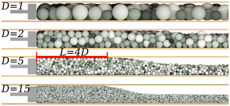
Figure 5. Particle positions for four simulations with varying gap spacing. Top to bottom: D = 1, 2, 5, and 15. For all cases, ϕ₀ ≈ 0.5, I = 0.01 and the simulation is displayed at the time corresponding to L = 4D. Particles are colored by size, darker colors representing smaller particles.

FIGURE 6

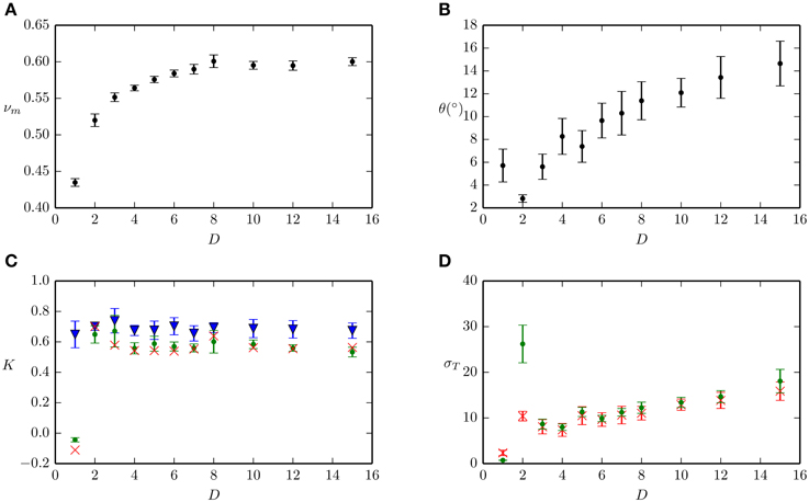
Figure 6. Descriptors of the system with varying gap spacing D. Error bars in each plot represent one standard deviation of the measured value. (A) Average solid fraction within the plug zone, ν_m. (B) Slope of the pile in the transition zone, θ. (C) Crosses represent best fit value of K_z from measurement of the stress on the piston head, σ^p_n using Equation (6). K_z and K_y, represented by dots and triangles respectively, are calculated directly from the coarse grained granular packing. (D) Threshold stress σ_T. Dots represent the mean value of the coarse grained continuum field σ_xx at x = L, and crosses represent predicted values from Equation (5) using measured values of ν_m, θ and ϕ₀.

For each simulation, the measured normal stress at the piston, σ^p_n, is fitted with Equation (6), and a best fit estimate of K_z is shown as crosses, with the standard deviation of the error of the regression used as error bars, in Figure 6C. The mean and standard deviation of the measured values of K_z and K_y from the continuum data between L = 2D and L = 10D are shown as dots and triangles, respectively. For D ≥ 2 we find that both the measured values of K_z and K_y are independent of D, and have mean values of K_y = 0.67 ± 0.04 and K_z = 0.58 ± 0.05. Best fit estimates of K_z are also independent of D, with mean values of K_z = 0.56 ± 0.07. Figure 6D shows the mean of σ_T also from L = 2 to L = 10. Triangles represent the prediction from Equation (5) using the measured values of ν_m, θ and ϕ₀. In all cases, we find the measured and fitted values of K_z to be in agreement, whereas the values of σ_T agree only with D ≥ 3. We note, however, that σ_T depends strongly on θ, and we have as yet no means for predicting this quantity. The dependence of σ_T on θ is in contrast to studies on fold and thrust belts [21], where there is no confinement vertically above the material.

3.2. Initial Packing Fraction

Existing models [8, 9] for the evolution of the stresses in similar geometries have neglected any effect of the initial packing fraction ϕ₀. To test this assumption, we here vary ϕ₀ from 0.1 to 0.6, while maintaining D = 5 and I = 0.01. As shown in Figures 7A,B, the packing fraction inside the plug and the slope of the transition zone are independent of the initial packing fraction. In Figure 7C, we observe that the measured and best fit values of K_z are in agreement for a wide range of ϕ₀, and that these values are lower than the measured values of K_y. The prediction of threshold stress from Equation (5), which includes a dependence on ϕ₀, slightly under-predicts the threshold stress at ϕ₀ = 0.1. Nevertheless, both the measured and predicted values of the threshold stress in Figure 7D are in agreement with observations from Eriksen et al. [8], where a non-dimensional threshold stress of σ_T = 10.7 was found to reproduce the observed pattern formation behavior in the quasi-static limit, at D = 5, for a range of values of ϕ₀ ≤ 0.5.

FIGURE 7

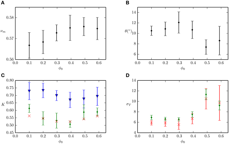
Figure 7. Descriptors of the system with varying initial packing fraction ϕ₀. Error bars in each plot represent one standard deviation of the measured value. (A) Average solid fraction within the plug zone, ν_m. (B) Slope of the pile in the transition zone, θ. (C) Crosses represent best fit value of K_z from measurement of the stress on the piston head, σ^p_n using Equation (6). K_z and K_y, represented by dots and triangles respectively, are calculated directly from the coarse grained granular packing. (D) Threshold stress σ_T. Dots represent the mean value of the coarse grained continuum field σ_xx at x = L, and crosses represent predicted values from Equation (5) using measured values of ν_m, θ and ϕ₀.

3.3. Inertial Number

Finally, we wish to comment on inertial effects in such a system. Toward this end we systematically vary the inertial number I from 10⁻² to 10 while maintaining D = 5 and ϕ₀ = 0.5 ± 0.05. As shown in Figure 8, a transition occurs at I ≈ 0.1, where the quasistatic behavior begins to be dominated by inertial effects, and the system is fluidized. In Figure 8A, we notice a jump in the maximum solid fraction, as the particles begin to flow and rearrange due to the increased piston velocity. This is accompanied by an increase in the slope angle θ (Figure 8B), and a decrease in the accumulation rate (Figure 8C, as the grains begin to slip relative to the walls. With increasing piston velocity, the anisotropy of the system is lost, as shown in Figure 8D, and both K_y and K_z tend toward a mean value of 0.56 ± 0.02 for I ≥ 1. As shown in Figure 8E, the threshold stress, σ_T, also diverges above I = 0.1 away from the theoretical prediction. For values of I ≥ 0.1, we have therefore used the measured value of σ_T in the best fit estimation of K_z shown in Figure 8D, rather than the value predicted from Equation (5), as used in all other cases.

FIGURE 8

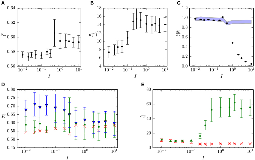
Figure 8. Descriptors of the system with varying inertial number I. Error bars in each plot represent one standard deviation of the measured value. (A) Average solid fraction within the plug zone, ν_m. (B) Slope of the pile in the transition zone, θ. (C) Slope of the best fit value of L(s) denoted by black dots against prediction using incompressibilty shown as the shaded region, which denotes ± one standard deviation around the mean value for each case. (D) Crosses represent best fit value of K_z from measurement of the stress on the piston head, σ^p_n using Equation (6). K_z and K_y, represented by dots and triangles respectively, are calculated directly from the coarse grained granular packing. (E) Threshold stress σ_T. Dots represent the mean value of the coarse grained continuum field σ_xx at x = L, and crosses represent predicted values from Equation (5) using measured values of ν_m, θ and ϕ₀.

4. Conclusions

We have here described a large number of simulations of granular materials which have been compacted in a confined geometry. For all cases, we observed that the stress distribution within the packing is well approximated by previous models, once a more rigorous definition of the threshold stress is used. This is true for a wide range of gap spacings, initial filling fractions and piston rates.

In this study we have used a rough boundary condition, where macroscopic friction at the piston and walls is equal to the inter-particle friction. However, in many systems we expect the roughness at the boundaries to be lower than that between particles. It is unclear how this difference will affect either the accumulation of material near the piston head, or the stress distribution within the packing.

Below a gap spacing of 3 particle diameters, the stress distribution is not well represented by this model. We conclude that D = 3 represents the smallest system size which may reasonably be described by the one dimensional Janssen stress model. In addition, at inertial numbers of I ≥ 0.1, we find that there is significant slip at the boundary, and the threshold stress diverges from the model prediction. In all cases, we cannot as yet predict the slope of the free surface in the transition zone, but we observe that this slope approaches the angle of repose for large systems at low piston rates. Janssen stress coefficients for this system are well represented by K_z = 0.6 ± 0.1 and K_y = 0.7 ± 0.1 for a wide range of system parameters. A model for the threshold stress has been presented using limit equilibrium, and this holds well for systems with D ≥ 3 and I < 0.1.

The slope angle, θ, has been measured for different system parameters to lie in the range of 2° – 18°. A priori, we could only assume that this angle must be smaller than or equal to the angle of repose, which for these grains is approximately 20°. The wide variability of θ is as yet unexplained, and is in contrast to the case where a top boundary does not exist, for example in fold and thrust belts [21], bulldozing [22] and additive manufacturing using loose powders [23]. We do note, however, that at large values of D the slope angle approaches the angle of repose.

With regards to the two Janssen parameters, we can clearly distinguish the values of K_y and K_z in Figures 6C, 7C, 8D, for I < 0.1. The reason for the difference between these two quantities may either be due to anisotropy in the granular packing, or due to the differing boundaries in the y and z directions. As the Janssen parameters are relatively insensitive to the gap spacing D, we conclude that this anisotropy is due to the accumulation process, which creates a preferential direction within the packing. This distinction is important when considering models which account for more complex geometries, such as in Eriksen et al. [8]. For industrial applications, such as propped fractures or sand production, the stresses within a plug of grains in a horizontal crack are expected to be a function not only of the relative size of the grains to the crack width, but also the rate of accumulation of the grains.

Author Contributions

BM conducted the simulations, post-processing and authored the paper. BS conceived the idea for the simulations. BS, GD, JE, and KM assisted with the interpretation and analysis of the simulations, and editing of the manuscript.

Conflict of Interest Statement

The authors declare that the research was conducted in the absence of any commercial or financial relationships that could be construed as a potential conflict of interest.

Acknowledgment

The authors would like to acknowledge grants 213462/F20 and 200041/S60 from the NFR.

References

1. Bräuer K, Pfitzner M, Krimer DO, Mayer M, Jiang Y, Liu M. Granular elasticity: stress distributions in silos and under point loads. Phys Rev E (2006) 74:061311. doi: 10.1103/PhysRevE.74.061311

CrossRef Full Text | Google Scholar

2. Landry JW, Grest GS, Silbert LE, Plimpton SJ. Confined granular packings: structure, stress, and forces. Phys Rev E (2003) 67:041303. doi: 10.1103/PhysRevE.67.041303

PubMed Abstract | CrossRef Full Text | Google Scholar

3. Sperl M. Experiments on corn pressure in silo cells–translation and comment of Janssen's paper from 1895. Granular Matter (2006) 8:59–65. doi: 10.1007/s10035-005-0224-z

CrossRef Full Text | Google Scholar

4. Janssen HA. Versuche über getreidedruck in silozellen. Zeitschr d Vereines Deutscher Ingenieure (1895) 39:1045–9.

Google Scholar

5. Tronvoll J, Fjaer E. Experimental study of sand production from perforation cavities. Int J Rock Mech Mining Sci Geomech Abstr. (1994) 31:393–410. doi: 10.1016/0148-9062(94)90144-9

CrossRef Full Text | Google Scholar

6. Veeken CAM, Davies DR, Kenter CJ, Kooijman AP. Sand production prediction review: developing an integrated approach. In: SPE Annual Technical Conference and Exhibition. Society of Petroleum Engineers. Dallas, TX, (1991). p. 335–46.

Google Scholar

7. Milton-Tayler D, Stephenson C, Asgian MI. Factors affecting the stability of proppant in propped fractures: results of a laboratory study. In: SPE Annual Technical Conference and Exhibition. Society of Petroleum Engineers. Dallas, TX, (1992). p. 569–79.

Google Scholar

8. Eriksen JA, Marks B, Sandnes B, Toussaint R. Bubbles breaking the wall: two-dimensional stress and stability analysis. Phys. Rev. E. (2015) 91:052204. doi: 10.1103/PhysRevE.91.052204

CrossRef Full Text

9. Knudsen HA, Sandnes B, Flekkøy EG, Måløy KJ. Granular labyrinth structures in confined geometries. Phys Rev E. (2008) 77:021301. doi: 10.1103/PhysRevE.77.021301

PubMed Abstract | CrossRef Full Text | Google Scholar

10. Sandnes B, Flekkøy EG, Knudsen HA, Måløy KJ, See H. Patterns and flow in frictional fluid dynamics. Nat Commun. (2011) 2:288. doi: 10.1038/ncomms1289

PubMed Abstract | CrossRef Full Text | Google Scholar

11. Sandnes B, Knudsen HA, Måløy KJ, Flekkøy EG. Labyrinth patterns in confined granular-fluid systems. Phys Rev Lett. (2007) 99:038001. doi: 10.1103/PhysRevLett.99.038001

PubMed Abstract | CrossRef Full Text | Google Scholar

12. Bratberg I, Måløy KJ, Hansen A. Validity of the Janssen law in narrow granular columns. Eur Phys J E (2005) 18:245–52. doi: 10.1140/epje/e2005-00030-1

PubMed Abstract | CrossRef Full Text | Google Scholar

13. Thornton AR, Weinhart T, Luding S, Bokhove O. Modeling of particle size segregation: calibration using the discrete particle method. Int J Modern Phys C (2012) 23:1240014. doi: 10.1142/S0129183112400141

CrossRef Full Text | Google Scholar

14. Weinhart T, Thornton AR, Luding S, Bokhove O. From discrete particles to continuum fields near a boundary. Granular Matter. (2012) 14:289–94. doi: 10.1007/s10035-012-0317-4

CrossRef Full Text | Google Scholar

15. Luding S. Cohesive, frictional powders: contact models for tension. Granular Matter (2008) 10:235–46. doi: 10.1007/s10035-008-0099-x

CrossRef Full Text | Google Scholar

16. Fuchs R, Weinhart T, Meyer J, Zhuang H, Staedler T, Jiang X, et al. Rolling, sliding and torsion of micron-sized silica particles: experimental, numerical and theoretical analysis. Granular Matter (2014) 16:281–97. doi: 10.1007/s10035-014-0481-9

CrossRef Full Text | Google Scholar

17. GDR MiDia. On dense granular flows. Eur Phys J E (2004) 14:341–65. doi: 10.1140/epje/i2003-10153-0

PubMed Abstract | CrossRef Full Text | Google Scholar

18. Goldhirsch I. Stress, stress asymmetry and couple stress: from discrete particles to continuous fields. Granular Matter (2010) 12:239–52. doi: 10.1007/s10035-010-0181-z

CrossRef Full Text | Google Scholar

19. Weinhart T, Hartkamp R, Thornton AR, Luding S. Coarse-grained local and objective continuum description of three-dimensional granular flows down an inclined surface. Phys Fluids (2013) 25:070605. doi: 10.1063/1.4812809

CrossRef Full Text | Google Scholar

20. Nedderman RM. Statics and Kinematics of Granular Materials. Cambridge: Cambridge University Press (2005).

Google Scholar

21. Davis D, Suppe J, Dahlen FA. Mechanics of fold-and-thrust belts and accretionary wedges. J Geophys Res. (1983) 88:1153–72. doi: 10.1029/JB088iB02p01153

CrossRef Full Text | Google Scholar

22. Sauret A, Balmforth NJ, Caulfield CP, McElwaine JN. Bulldozing of granular material. J Fluid Mech. (2014) 748:143–74. doi: 10.1017/jfm.2014.181

CrossRef Full Text | Google Scholar

23. Parteli EJR. DEM simulation of particles of complex shapes using the multisphere method: application for additive manufacturing. AIP Conf Proc. (2013) 1542:185–8. doi: 10.1063/1.4811898

CrossRef Full Text | Google Scholar