Bridging aero-fracture evolution with the characteristics of the acoustic emissions in a porous medium

1. Introduction

Fluid flow [1, 2], rock deformation [3] and granular dynamics [4] by themselves are very large scientific domains to investigate individually [5]. However, the idea of putting them together via a system of deformable porous medium with a fluid flow makes the phenomena even harder to understand. Rapid changes in the porosity of the medium due to fluid flow, channeling and fracturing via momentum exchange with the flow make understanding the mechanics of the system a challenge [6–9]. Hydraulic fracturing of the ground is a good example for this coupled behavior of solid and fluid phases. First, the pressure of the flow creates fissures and cracks which changes the permeability of the initial rock. Then, a flowing mixture of fine sand and chemicals helps maintain this cracked state by penetrating the newly opened areas. By jamming and/or cementing the newly-formed channels and cracks, possible relaxation after injection is prevented. Thus, a more permeable state of the rock is preserved after injection for various types of industrial applications. Recently, various well-stimulation projects have attempted to use pressurized gas (N₂, CO₂), instead of water, to trigger fracturing within reservoirs for several reasons (e.g., to avoid wasting water, to sequestrate CO₂, environmental risks due to chemicals etc.) [10–12]. In this study, contrary to conventional fracturing methods, the fractures are induced using air injection.

Monitoring, predicting and controlling fracture evolution during hydraulic-fracturing, steam-assisted gravity drainage, or CO₂ sequestration operations is a key goal [13–16]. One possibility for monitoring is to use generated acoustic emissions during those operations. In the hydraulic fracturing industry, the typical monitoring devices consist of geophones and seismometers. However, the interpretation of the signals during fast deformations of porous media due to fast fluid flow is not simple. Particularly, the measurements of deformations are usually difficult to achieve in an opaque medium, and the source of the seismic waves and acoustic emissions can be complex. The study of microseismicity during well operations is routinely done in the industry, but its interpretation is often delicate [17–19].

In this paper, we present an experimental study using a purpose-built setup allowing channeling and fracturing due to fluid flow, where we can observe the deformations optically using a fast camera and transparent setup, and simultaneously record the mechanical waves emitted by the complex channels and fractures created. Both signals, optical and acoustic/microseismic, are then analyzed. They display a complex evolution of the source geometry, and of the spectral characteristics. The experimental setup designed to achieve this consists of a rectangular Hele-Shaw cell filled with 80 microns diameter grains, mixed with fluid (air). The linear cell has three lateral sealed boundaries and a semi-permeable one enabling fluid (but not solid) flow. During the experiments, air is injected into the system from the side opposite to the semi-permeable boundary so that the air penetrates into the solid and at high injection pressures makes a way to the semi-permeable boundary via the creation of channels and fractures - or at low injection pressures, directly using the pore network.

For a similar system of aerofractures in a Hele-Shaw cell, a numerical model was conducted by Niebling et al. [20]. These models were also compared with experiments for further development and validation [20–24]. Same kind of experiments—but without acoustic monitoring—with a Hele-Shaw cell have also been conducted. Johnsen et al. worked on the coupled behavior by air injection into the porous material both in fluid saturated and non-saturated cases to study multiphase flow numerically and experimentally [23, 25, 26]. Aero-granular coupling in a free falling porous medium in a vertical Hele-Shaw cell was studied numerically and experimentally by Vinningland et al. [27–29]. Varas et al. conducted experiments of air injection into the saturated porous media in a Hele-Shaw cell [30, 31] and in a cylinder box [32]. Eriksen et al. and McMinn et al. worked on injecting gas into a saturated deformable porous medium [Eriksen et al., submitted; 33]. Sandnes et al. classified different regimes of fingering of porous media in a Hele-Shaw cell [34]. Rust et al. developed a closed-system degassing model using volcanic eruption data [35]. Holtzman et al. also studied air induced fracturing where they identified different invasion regimes [36]. Furthermore, a recent study was conducted by Eriksen et al. where the air injection causes bubbles in a fluid-grain mixture [37].

The equivalent of microseismicity monitoring in the lab is the tracking of acoustic events. Hall et al. compared recorded acoustic emissions with the digital image correlation to track crack propagation in the rock samples [38]. Valès et al. used acoustic emissions to track strain heterogeneities in Argilite rocks [39]. Some studies have started to look at sources directly, both optically and acoustically, in various problems to characterize the different source mechanisms [40–44]. Farin et al. conducted some experimental studies on rockfalls and avalanches where he monitors those phenomena using acoustic emissions [45]. Stojanova et al. worked on fracture of paper using acoustic emissions created during crack propagation [46–48]. During the current experiments, acoustic signals are recorded using different sensors (shock accelerometers and piezoelectric sensors). Those signals are compared and investigated further in both time and frequency domains. Furthermore, during the experiments, photos of the Hele-Shaw cell are taken using a high speed camera. Thus, it is possible to visualize the complex branched patterns arising due to the solid-fluid interaction and to process images to gather information about the strain and strain rates, and investigate the mechanical properties of the solid partition.

2. Experimental Setup

A Hele-Shaw cell is made of two glass plates (80 × 40 cm) placed on top of the other, separated by 1.5 mm distance. The plates are separated via aluminum spacers placed close to the edges to provide equidistant spacing across the cell. For the experiments particular to this study, we completely sealed three boundaries of the Hele-Shaw cell and made one semi-permeable boundary using 50 μm steel mesh which allows fluid to exit the system but keeps the solid grains inside the cell. One of the plates has an inlet, which is used for injection of pressurized air, located at the bottom end of the plate, midway from the long edges 3 cm inside from one of the clamps close to the shorter edge (Figure 1A). The cell is filled with non-expanded polystyrene grains (80 μm diameter ±1%) called Ugelstad spheres (see details in Toussaint et al. [49]). The density of the spheres is 1.005 g/cm³. A mass of 170 g of grains is required to fill the cell, corresponding to an initial solid fraction of 52 ± 5% which is close to the 57% random loose pack for monodispersed grains [50]. Solid fraction of the grains in similar systems was investigated thoroughly by Johnsen et al. and found to be as low as 44% [23]. The difference between our experimental value and the theoretical value for an infinite box could be due to finite size of the cell which causes steric effect between the grains and the flat boundaries of the container, making the solid fraction 10–15% less [51]. Additionally, the measurement of 1.5 mm plate separation is subject to an error of 10% which has a direct effect on the solid fraction error bar. Electrostatic forces and humidity are also effective for real experimental beads and not for theoretical hard spheres, which can lower the solid fraction.

FIGURE 1

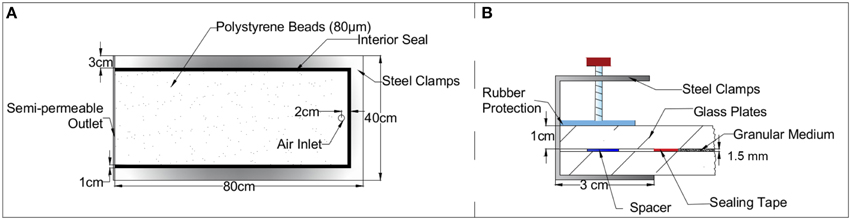
Figure 1. Schematic diagram of the Hele-Shaw cell including the dimensions. (A) Top view of the Hele-Shaw cell including its dimensions. The cell is made of two glass plates which are placed on top of the other with 1.5 mm spacing between them. A porous medium is placed inside the cell. Three sides of the cell are sealed and the 4th boundary is sealed with a semi-permeable filter. (B) Side view of the Hele-Shaw cell showing clamp details. To protect the glass plates from point loading, a rubber sheet is placed in between the screw and the plate. Aluminum spacers are placed in between the plates to provide equivalent spacing everywhere in the cell.

Some of the grains are colored with Indian ink to provide markers and texture, allowing a better resolution of the displacement measurements based on optical data. Images taken via high speed camera are used for digital image correlation to have full field measurements of displacement, velocity, strain rate etc. [21, 52–54]. The solid-air interface is placed 1-2 cm away from the inlet to avoid pressure localization close to the inlet. A schematic diagram of the Hele-Shaw cell is shown in Figure 1. The sides of the Hele-Shaw cell are clamped using steel clamps after sealing with double-sided rubber sealing tape. To protect the glass plates from stress focus on the clamping points, rubber sheets are placed between the clamp screws and the glass plates. Before placing the semi-permeable boundary, the cell is placed vertically and grains are poured inside. Following this, a semi-permeable filter is placed on the 4th edge. Then, the Hele-Shaw cell is positioned vertically, in a way that the semi-permeable boundary stays at the bottom side to decompact grains and homogenize the solid fraction through the cell. Another important goal of this rotation process is to provide a small rectangular buffer empty of grains around the air injection inlet to avoid having point injection force over the medium. After the filling phase, the Hele-Shaw cell is placed horizontally.

Air injection is started and ceased via an electrovalve placed on the pipe very close to the air inlet, (Figure 2). This air pressure is provided via a pressurized air tank. Injection pressure over time is constant. It starts like a step function and is monitored using a pressure sensor placed on the air inlet allowing to check if the real injection pressure is within 5% of the value required during the experiment.

FIGURE 2

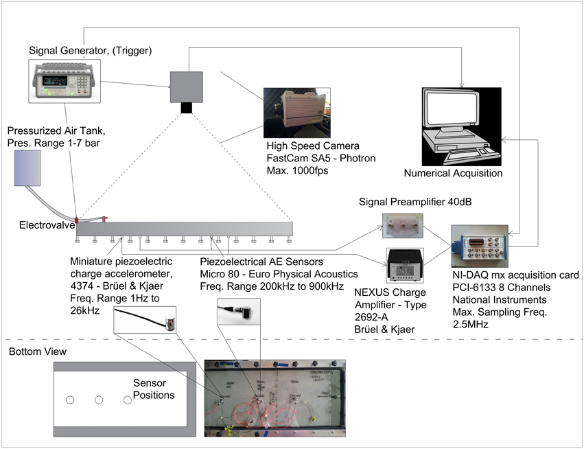
Figure 2. The acquisition chain of the aero-fracturing experiments with a Hele-Shaw cell. The signal acquisition card, camera and the electrovalve connected to the air pump are triggered at the same time via a TTL sent from the signal generator to have synchronized optical and acoustic data. The sensors are placed on the bottom glass plate of the Hele-Shaw cell.

During the experiments, acoustic signals are recorded using different sensors. The data recorded on the piezoelectric sensors which are mostly sensitive in the range (200–900 kHz) are amplified with a Signal Preamplifier. The data recorded on the shock accelerometers which are mostly sensitive in the range (1 Hz–26 kHz) are amplified with a Brüel and Kjaer Nexus Charge Amplifier—Type 2692-A. The amplified/conditioned signal is transmitted to the computer via a Ni-DAQ mx PCI-6133 acquisition card with multiple channels at 1 MHz sampling rate (Figure 2). In addition, synchronized with the acoustical data, images of the Hele-Shaw cell are taken via a Photron SA5 high speed camera transferred and stored numerically. A TTL signal is used as a trigger to initiate the injection and the data acquisition via the camera and the acoustic sensors, thus, enabling time synchronization between the apparatus. Ambient lab noise is also recorded for reference and investigated using camera and accelerometer recordings prior to air injection. After recording, the signals are corrected by using the response function of the accelerometers provided by the manufacturer and cross-checked at the lab.

3. Experimental Observations

At large enough injection pressures, the fluid makes its way by creating channels and fractures toward the semi-permeable boundary as seen in Figure 3. In the beginning, the solid-air interface of the porous medium (closest to the injection point) moves more or less homogeneously, with the appearance of only large scale curvature of the interface (Figure 3B). Then after roughly 150 ms, some thin finger-like carved formations of thickness around 2 mm start to appear at several points (marked with yellow circles in Figure 3C). As injection continues, those fingers penetrate further in the medium. They get larger and wider with the help of the air pressure (Figure 3D). In addition to that enlargement, fingers branch out into thinner fingers. In the end, a tree-like branched channel network is created inside the porous medium. As a result of those fractures and channels, the surrounding material is displaced and the porous medium is compacted. Fracturing, channeling and fluid interaction inside the porous medium has its effects on the granular part of the medium. These interactions also result in granular transportation and compaction which involves inter-granular interactions as well as interactions of the solid grains with the confining glass plates. Initially the solid fraction is homogenous inside the plate. However, during the experiment the solid fraction of the grains increases in the close vicinity of the channels and fractures (up to the maximum possible solid fraction up to 63% for loose packed medium [50]. As observed in numerical models of such system in Niebling et al. [24], this solid fraction may decrease with distance from the fingers. After the experiment, depending on the pressure duration, initial solid fraction, and overpressure, some parts of the medium may have remained at the initial solid fraction, in other words may not have been compacted at all.

FIGURE 3

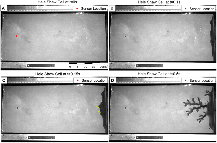
Figure 3. Image of the Hele-Shaw Cell prior to injection (A), during quasi-homogenous compaction (B) and during channeling (C–D). Red dot shows the position of the acoustic sensor (accelerometer). Yellow circles in (C) represent the locations of the first finger-like carved formations.

The acoustic events recorded during the experiments arise presumably due to sources of various types. While some vibrations are happening solely due to the air pressure fluctuation inside the channels, some others are generated by the stress increases on the plates due to granular compaction, intra-porous air pressure vibrations, granular shocks and variation of the friction forces. These sources excite the confining plates, transporting mechanical waves to the sensors, i.e., the source types that are convoluted with the response of the Hele Shaw cell structure. Eventually, what is recorded is not just a signal created by a simple source, but a systemic response (i.e., signals interacting with plates and clamps, reflecting from edges, refracting through interfaces and eventually having different characteristic properties) to the many individual processes happening inside the plate during the whole period of the experiment. Signature of the signals recorded during experiments did not depend significantly of the sensor type and location.

Even though many individual acoustic events are superposed in time in the recorded signals, and are influenced by a systemic response, this does not mean that their specific signature is lost. Superposed signals may hide their signatures in the time domain, however their influence in the power spectrum may still be noticeable. In the following section, the evolution of the power spectral signature with varying solid-fluid interactions (e.g., compaction of the solid with fluid pressure, channeling, diffusion of the overpressure of the injected fluid through the pore spaces etc.) is shown. First, the power spectrum of several snapshots in time (i.e., Fast Fourier Transform, FFT), taken from different experimental stages, are presented. Then, they are analyzed and compared with each other. The flowchart in Figure 4 describes the analysis procedure.

FIGURE 4

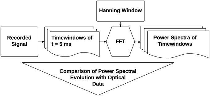
Figure 4. Flowchart showing the acoustic-emission analysis procedure. Snapshots of the experimental signal is taken. Then, they are first converted to the fourier domain to obtain the power spectra. Afterwards, power spectra are compared with each other to understand differences.

4. Results

4.1. Power Spectral Evolution

The first time window analyzed, occurred prior to injection (i.e., at a state of rest). Figure 3 shows an image of the Hele-Shaw cell, acquired via the fast speed camera. The acoustic recordings at the same time step are shown in Figure 5. The air injection starts at t = 0 s.

FIGURE 5

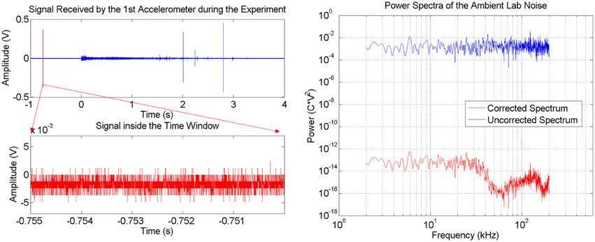
Figure 5. Ambient Lab Noise recorded prior to experiment. The red strip in the top left panel (time window of 0.005 s) and its zoomed version (Bottom left panel) corresponds to the snapshot that the power spectra (Right) occurred at. Right panel: The uncorrected (blue) and corrected with sensor response (red) power spectra of the ambient lab noise.

Before injection, only ambient electrical noise in the recording system is present. Its power spectrum is flat (Figure 5, Right, Blue Curve). After correction with the sensor response the mechanical response (Figure 5, Right, Red Curve) is obtained. This noise represents the minimum mechanical vibration level which can be captured by the sensors without being hidden by the electrical noise. Aside from the ambient noise within the lab, no other signal is present. The red strip (time window of 0.005 s) on the experimental signal (Figure 5, Top-Left) shows the time window of signal when the picture in Figure 3A is taken. The FFT is applied to this time window to obtain the power spectrum which is presented in the right panel of Figure 5.

Compaction starts when the fluid (air) pressure is sufficiently large to move the solid grains. In Figure 6A, 150 ms after the start of the injection, channel initiation can be observed at several points, as highlighted by the yellow circles. Due to the interaction between the solid and fluid phases inside the Hele-Shaw cell, some mechanical signals are generated. The power spectrum of the signal recorded during this snapshot is presented in the bottom right panel of Figure 6. As channeling continues, the bulk movement of the grains takes place together with fluid motion. This causes emergent acoustic emissions which are predominantly in the low frequency range (less than 10 kHz). Vibration of the plates, granular friction and stress differences on the plates due to compaction create waves that are also in the power spectrum. All those contributions from different source mechanics gives a shape to the presented power spectra, similar to a power law decay having an exponent b = −1.61.

FIGURE 6

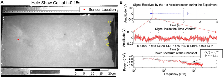
Figure 6. Optical (A) and acoustic (B) experimental recordings just before channeling. Yellow circles on the left image shows the initiation points of the channeling. The red dot on the left image illustrates the sensor location where the signal on the right is recorded. Top Right panel: Acoustic signal recorded throughout the entire experiment. The red strip (time window of 0.005 s) corresponds to the snapshot that the image (A) and power spectrum (Bottom Right) occurred at.

In addition to this slope, it is possible to find the mean frequency of the power spectra using Equation (1).

$\begin{array}{ll}\langle f\rangle =\frac{\int f|a(f){|}^{2}df}{\int |a(f){|}^{2}df}& (1)\end{array}$

This will show the dominant frequency range within the signal. In the following Figure 7, it can be seen that the mean frequency starts very low and then increases with increasing energy in the high frequency range. As the channel network develops, we see that the mean frequency reaches to its maximum value. Using cubic fitting, this mean frequency curve is estimated and compared with the optically obtained curves. An inflection point of the fitted curve is observed around time t₀ = 1.49 s after injection. This corresponds to the point where the finger development stops and the regime inside the Hele-Shaw cell changes to a slow relaxation stage with slow fluid overpressure diffusion detailed in the discussion section.

FIGURE 7

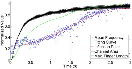
Figure 7. Mean frequency evolution (normalized with the maximum value 200 kHz) during injection. As the channel network develops progressively the energy percentage in the low frequency range f < 10 kHz diminishes, and the mean frequency gets higher. A cubic polynomial curve (red) is fitted to the mean frequency data to simplify the comparison and discussions. The location of the inflection point of this curve is indicated by the (red) dash dot strip (t₀ = 1.49 s). In this curve the normalized maximum finger length (green, maximum value is approximately 35 cm) and the carved area (black, maximum value is approximately 270 cm²) is also presented. The area saturates to a maximum at a time close to t₀. The length still increases slightly after t₀, in particular, a small step in finger length (high slope of the length curve, corresponding to a large stick slip event connected to the finger) can be noticed around t₀.

4.2. Acoustic Events

It is possible to link the information received from the small scale lab experiments with large scale data, and vice-versa. In the experiments, we noted that the number of acoustic events occurring inside the Hele-Shaw cell is related to the empty channel area. However, after the fractured area reaches the final channel network shape, stress relaxation events are observed. These events are investigated further using event counting methods based on the ratio of Short Term Average over Long Term Average (STA/LTA) for event detection and compared with the evolution of the channel area inside the Hele-Shaw cell.

4.2.1. Event Detection

Detecting the number of events occurring during fracturing is a good indicator of the compaction level within the material. As long as there is motion of granular particles with the fast fluid flow it is very probable to detect some acoustic events in the experimental recording. However, it is very important to analyze and understand which part of the recording can be labeled an event and which part can not. STA/LTA threshold method is commonly used in seismic data interpretation [55–58]. If the parameters are selected carefully, it is very easy to use and is very robust [59]. While LTA considers the average temporal noise to have an idea of the general behavior of the site, STA looks for intense changes in the signal in a small time window to detect acoustic events. Thus, it makes the ratio of those two parameters sensitive to the more complex events as well. When this STA/LTA ratio passes a pre-defined threshold, it is considered as an event (Figure 8), and the event counter is incremented. As long as the ratio stays above the threshold, it does not trigger again. Right after the ratio goes below the threshold, the algorithm can be triggered again for the next event to be counted. This algorithm (for one time window) can be generalized as follows:

$\begin{array}{cc}\frac{(STA)}{(LTA)}=\frac{\frac{1}{N_s}{\displaystyle {\sum }_i^{i+N_s}(s(}i{)}^2)}{\frac{1}{N_l}{\displaystyle {\sum }_i^{i+N_l}(s(}i{)}^2)}\hfill & (2)\hfill \end{array}$

$\begin{array}{rcll}\text{Ψ}\hfill & =\hfill & \frac{(STA)}{(LTA)}\to \text{Ψ}>T\to Event\hfill & (3)\hfill \end{array}$

where s(i)² is the squared raw signal in the time domain (if necessary, a filtered signal s′(i)² can be used for different characteristic events), N_s and N_l are the length of the short (0.05 ms) and long time (1 ms) windows respectively and T is the predefined threshold for an event. The threshold to detect events may change between different datasets or different types of acoustic events.

FIGURE 8

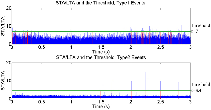
Figure 8. STA/LTA detection plots for Type 1 (upper figure) and Type 2 (lower figure) events. Top: The raw signal is filtered by using a butterworth bandpass filter with corner frequencies 100 Hz and 10 kHz before computation. Bottom: The raw signal is filtered by using a highpass filter for frequencies higher than 100 kHz before computation. We found that some of the Type 2 events can be classified as Type 1 events since they have energy in the low frequency higher than the threshold.

4.2.2. Event Classification

One important thing that should be mentioned about the STA/LTA counting method is the frequency range used. After detailed analysis, it has become apparent that two different types of events exist within the experimental dataset. The first type of events are the non-impulsive low frequency (less than 10 kHz, similar to Figure 6) events (Type 1) which are related to the fluid flow and to the fluid-grain interactions rearranging the grains and producing major deformations and channeling. These events begin at the moment when the air injection starts and continue until a fully developed channel network is reached. It is possible to determine accurately this period from the optically acquired data, simply by calculating the area of the channel (estimated via the number of dark pixels in a binarized image) that saturates to a maximum value before the end of the acoustic emissions. Interestingly, in our findings, the number of Type 1 acoustic events follows a similar trend in time as the evolving emptied channel area within the Hele-Shaw cell (Figure 9). To enable the detection algorithm to distinguish between the different types of events, frequency filters are applied. To detect Type 1 events, a butterworth bandpass filter with corner frequencies 100 Hz and 10 kHz is applied to the raw signal s(i) before the STA/LTA event detection is applied.

FIGURE 9

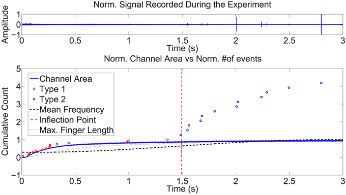
Figure 9. Top: Signal recorded during the experiment. Bottom: Blue curve shows dark pixel counting over the image to compare compacted area with the number of different acoustic events occurred. Circles represent cumulative number of events normalized with maximum number of Type 1 events (i.e., 17 events). Cumulative number of Type 1 events (red points) are fitting well to the normalized channel area with time presented in the lower plot. First Type 2 (blue) event occurs very close to the inflection point of the mean frequency curve. Type 2 events are very impulsive and noticeable in the top panel as well.

The second type is the aftershock-like events, Type 2. Unlike the Type 1 events, in power spectrum their energy is spread over a wide frequency range similar to the one presented in Figure 10. These events are similar to the stick-slip relaxation events following a big earthquake in real scale. Compacted grains are rearranging their positions to have a more compacted state due to continuous air injection which results in some of their energy being released as acoustic emissions. To detect Type 2 events, a highpass filter for frequencies higher than 100 kHz is applied to the raw signal s(i) before the STA/LTA event detection is applied. In Figure 11 the evolution in the power spectrum with time is presented. In the figure, a Type 2 event occurred at t = 2.8 s is also presented.

FIGURE 10

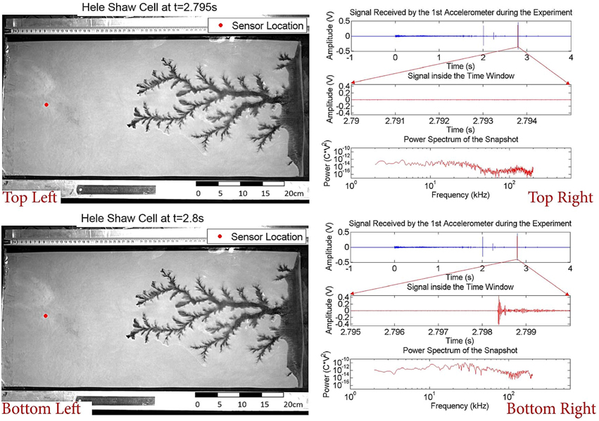
Figure 10. Optical (Left) and acoustic (Right) experimental recordings just before (Top) and during (Bottom) an aftershock like event. The red dot on the left image illustrates the sensor location where the signal on the right is recorded. Top Right: Acoustic signal recorded throughout the entire experiment. The red strip (time window of 0.005 s) corresponds to the snapshot that the image (Left) and power spectrum (Right) occurred at.

FIGURE 11

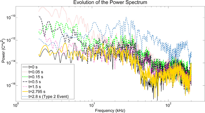
Figure 11. The evolution of power spectrum over different time windows are presented. With time, the power is decreasing until finally reaching back to the initial level. However, during Type 2 events the spectrum has a completely different signature.

After investigating further, we also noticed that the occurrence frequency of these events decay with time, similar to the Omori Law [60, 61]. In the following section, curve fitting to the number of Type 2 acoustic emissions assuming an Omori Law decay (Figure 12) will be discussed.

FIGURE 12

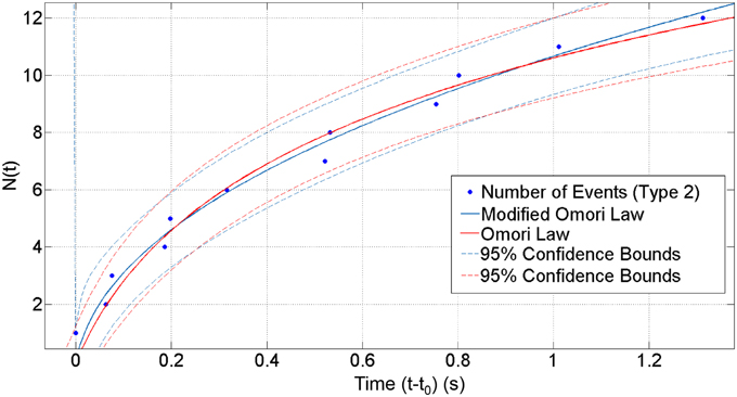
Figure 12. Conventional and Modified Omori Law Fits of the cumulative number of events. The circles represent the cumulative number of events and the solid lines represent the fitting curves given by the Equations (5) and (7). t′ = 0 in this representation corresponds to time t₀ = 1.49 s after the start of the air injection.

4.2.3. Omori Law

Omori [60, 61] worked on the half-day and monthly frequencies of aftershocks of the 1891 Nobi earthquake in Japan [60, 61]. He found that the frequency of aftershocks n(t′) at time t′ can be expressed as:

$\begin{array}{ll}n(t^{\prime })=K{(t^{\prime }+c)}^{-1}& (4)\end{array}$

and the same equation for the cumulative number of aftershocks is given as

$\begin{array}{cc}N(t^{\prime })={\displaystyle {\int }_0^{t^{\prime }}n}(s)ds=Kln(t^{\prime }/c+1),& (5)\end{array}$

where c is a characteristic time, small and positive, K is the slope of the fit in the semi-logarithmic domain and N(t′) is the number of cumulative aftershocks up to time t′. Following Omori, Utsu (1957) emphasized that the real aftershock activity decays with time differently than the originally derived Omori Law and proposed the equation for the frequency of aftershocks, with another fitting exponent p, as Utsu [62, 63]:

$\begin{array}{ll}n(t^{\prime })=K^{\prime }{(t^{\prime }+c^{\prime })}^{-p}& (6)\end{array}$

and called this the Modified Omori Law (MOL). The corresponding equation for the cumulative number of aftershocks is given as:

$\begin{array}{cc}N(t^{\prime })=\frac{K^{\prime }}{(p-1)}({c^{\prime }}^{1-p}-{(t^{\prime }+c^{\prime })}^{1-p})& (7)\end{array}$

where c′ is a characteristic time and K′ is the slope having the dimension of time^(p−1).

Using these approaches Omori Parameters K, c and p are estimated on our experimental catalog of Type 2 events, using time t′ = t − t₀, where t₀ is the time defined in Section 4.1, that corresponds to the end of the channel formation and to the inflection point of the mean frequency recorded (Figure 12). A bin size to find frequency of occurrence of the events is selected as 0.2 s. However, it is more robust to use cumulative number of aftershocks (Equations 5 and 7) to avoid choosing an additional parameter for binning which can vary. Fitting is computed with 95% confidence bounds (i.e., two standard deviations away from the mean of the estimated value) to show the quality of fitting. Fitting parameters are calculated by a linear regression in the semi-logarithmic space of the cumulative number of events as K = 4.89 ± 1.33 and c = 0.13 ± 0.8 s. The Root Mean Square Error (RMSE) - average of the residual of the fit - is calculated to be 0.57 in this particular fit using the Equation (5).

Using the Modified Omori Law (i.e., Equation 7) fitting parameters are found as K′ = 5.34 ± 1.52 s^−0.45, c′ = 0.0066 ± 0.55 s, p = 0.55 ± 0.38 and RMSE is calculated to be 0.53 and the error bar is evaluated as the standard error [64]. The dashed lines in the Figure 12 represents two RMSE from the fitted curves.

5. Discussion

5.1. Discussion of the Experimental Results

The power spectrum of the mechanical signal at the different time windows show that the interactions inside the Hele-Shaw cell are evolving with continuous injection. In the beginning, there is a bulk movement of the grains due to the compaction caused by air injection. In Figure 6B it can be seen that the power spectrum follows a power law trend with an exponent equal to −1.61 without any major peak. This indicates, although there are many different phenomena with various characteristic frequencies happening at the same time (e.g., bulk compaction, interactions between solid and fluid phase, stress redistribution among the medium etc.), that a scale-free mechanical phenomenon—probably related to the developing branching pattern—is dominating the emissions. Since the low frequency has higher energy, it can be seen that the mean frequency of the initial part t < 1.5 s is low as well (Figure 7). As the channeling and fingering starts, the mean frequency is shifting from lower frequencies f < 10 kHz to the higher frequencies. Moreover, this evolution can be seen in Figure 11. Rising mean frequency is also seen in the signals recorded during some volcanic processes, as e.g., the 2004 eruption process of the Arenal volcano, Costa Rica, and was interpreted as related to the stress increase with time due to the fluid pressure [65]. Additionally, the rate of this increase decreases as the channel network establishes. The trend which represents the channel area and also increasing permeability due to fracturing, is given in Figure 9 by checking the dark pixels in the images through time. Occurrence frequency of low frequency earthquake-like events (described as Type 1) decreases with increased permeability due to fingering and fracturing indicated in the work of Frank et al. about real scale events seen in Mexico [66].

The inflection point (Figure 7 red dash dot line) of the mean frequency curve (t₀ = 1.49 s) shows the point where the power spectra evolves from a power law trend (Figure 6B) to stick-slip aftershock like events (Figure 10, Bottom Right) whose power spectra consists of several peaks in the frequencies higher than 10 kHz (Figure 11) which causes the increase in the mean frequency. This inflection point occurs almost at the same time as the small step in the maximum finger length curve (high slope of the length curve, Figure 7 green) can be noticed around t₀. This small step shows a stick slip motion in the most advanced finger tip. The inflection point also corresponds to the start of occurrence of the first Type 2 event which is presented in Figure 9. We can thus attribute it to a change in dynamics of the pneumatic fracture process: the main tree of channels stabilizes, and a slower stress relaxation process starts in the bulk around the channels, which leads to different type of acoustic event signatures, associated to the appearance of the impulsive Type 2 events.

The presence of this inflection point in the average frequency of the power spectrum, and the appearance of impulsive events (Type 2), can be suggested as the interesting signatures of the stabilization of the main channel during the monitoring of field scale hydrofracture or pneumatic fracture: these clear signatures can be detectable even in opaque field scale microseismic monitoring studies. This change of event types can also be seen in Figure 9 which shows the event detection using STA/LTA event detection procedure. As presented in the bottom panel of Figure 8, Type 2 events are detected starting from the inflection point of the mean frequency curve (t₀ = 1.49 s). Furthermore, we noticed that the cumulative number of Type 2 events are following an Omori Law trend which is shown in the Figure 12. This is due to the similarity between the aftershocks which is observed in real life and the Type 2 events in the medium which are due to the local stress relaxations. K = 4.89 ± 1.33 and c = 0.13 ± 0.8 s for the Omori Law and K′ = 5.34 ± 1.52 s^−0.45, c′ = 0.0066 ± 0.55 s, p = 0.55 ± 0.38 for the Modified Omori Law are computed as fitting parameters. It can be said that the Modified Omori Law—Equation (7)—gives slightly better fitting results to this dataset (RMSE is 0.57 for Omori Law and 0.53 for Modified Omori Law) due to the application of another parameter which is making the fitting procedure more sensitive.

The obtained p-value in this study (p = 0.55) corresponds to the p-value range for earthquakes studied by different scientists (i.e., 0.6–1.6 [63], or 0.3–2.0 [67]). There are several studies for different types of earthquake mechanisms with varying p-values. Utsu [63] presented some of them: p = 0.9 ± 0.1 is found for the 1962 Westport earthquake in New Zealand, p = 1.4 is found for the 1965 Hindu Kush intermediate-depth (h = 214 km) earthquake, and p = 0.84 is found for the aftershocks following a rock fracture event in a mine causing a low magnitude earthquake (M = −2). This variability has been attributed to the variations in the state of stress, temperature, structural heterogeneities, material parameters, etc., in different tectonic regimes. However, a single, dominant factor controlling this parameter has not yet been identified [68].

In different examples, post-injection fluid-induced seismic events at various injection sites such as Fenton Hill, USA, and Soultz-sous-Forêts, France, appear to decay with an Omori-like fashion [69]. The rate of the post-injection seismic events in these cases has not been analyzed using the conventional MOL, thus a direct comparison between the obtained p-values cannot be carried out. In other examples, Nur and Booker [70] found that the decay of earthquakes following a step in the pore fluid pressure obeys a Modified Omori Law (MOL) with p = 0.5, which was consistent with a pore fluid diffusion law. Similarly, Yamashita worked on a model linking the fault slip and fluid flow in a system preloaded in shear. He found that the p-value is 0.48 for an early time period in a sequence of induced secondary aftershocks [71]. This link was also derived by Shapiro et al. [72–74] and Rozhko et al. [75] for the events related to pressure changes in operation wells. Their formulation relates the rate of acoustic events to the temporal change in pore pressure. This is very similar to the p-value obtained by fitting the MOL to our experimental results.

5.2. Physical Explanation of the Experiments

The observed p-value in our experiments is also consistent with the derivations and approximations carried out in the models derived by Niebling et al. [20, 24] or Johnsen et al. [25] for systems related to the one currently studied. The exponent of this Modified Omori Law and its prefactor can be directly related to the stress relaxation due to the diffusion of fluid pressure with the following approximations - that will be validated a posteriori by the agreement between the exponent and prefactor derived and the one that can be measured directly.

After the initial fast stage where the large empty channel is created, the compressibility of the fluid induces a slower seepage into the surrounding material. The boundary conditions can be considered as fixed for the granular material along the channel: owing to the large permeability of the channel, the boundary condition along the channel corresponds to an approximately homogeneous fluid pressure equal to the imposed inlet pressure, which also corresponds to the total stress since no grains are present in the channel, and the total pressure and pore pressure correspond on this boundary. The outlet boundary conditions can be considered as fixed pore pressure equal to the atmospheric one, and fixed displacement due to the semipermeable grid. The boundary conditions along the plates correspond to no flux for the fluid, and no normal displacement for the particles.

Since no large motion occurs in the following relaxation stage, the total stress field in the medium can be approximated as constant. This total stress σ^T is the sum of the solid stress σ^s arising from the forces transmitted in the grain-grain and grain-plate contacts, and the pore pressure p:

$\begin{array}{ll}{\sigma }^T={\sigma }^s+\mathrm{pId},& (8)\end{array}$

where Id is the identity matrix. This general formulation of summing the solid-bearing and fluid-bearing parts of the stress is for example demonstrated by Jackson [76], and is valid as long as the large scale shear stress due to fluid-solid momentum exchange is negligible. It was shown to hold, for example, in sheared saturated granular layers [77].

The total stress being fixed with fixed boundary conditions, the balance between solid-bearing and fluid-bearing stress changes as the fluid seeps in due to pore pressure relaxation. For every grain-grain contact and grain-plate contact, the stick/slip criterion can be described using a Coulomb friction criterion according to which slip occurs when the equality is reached:

$\begin{array}{ll}{\sigma }_s^s\ge \mu {\sigma }_n^s,& (9)\end{array}$

where ${\sigma }_n^s$ and ${\sigma }_s^s$ are respectively the norms of the normal and shear (frictional) solid stress transmitted by the contact considered, and μ is the friction coefficient depending on the characteristics of the contacting elements (grains and plates).

The fluid can be explicitly considered by expressing this law in terms of total stress and fluid pressure, using Equations (8, 9) which leads to a formulation corresponding to Terzaghi's 1936 effective stress formulation [77, 78]:

$\begin{array}{ll}{\sigma }_s^T\ge \mu ({\sigma }_n^T-p),& (10)\end{array}$

where p is the pore fluid pressure. With fixed total stress, Equation (10) can be reformulated in terms of fluid pressure required for the grain pairs to slide:

$\begin{array}{ll}p>{\sigma }_n^T-\frac{{\sigma }_s^T}{\mu }.& (11)\end{array}$

We assume a random distribution for the local total stress values, ${\sigma }_s^T$ and ${\sigma }_n^T$, and call ξ the density of contacts per unit surface of the plates that will break with an acoustic emission due to sufficiently high pore fluid pressure. According to the above criterion, when p rises from the initial value to the final one a slip, during which micro acoustic events are produced, happens. The rate of events can be derived as follows: the system is considered to have a quasi one dimensional geometry where the grains ahead of the channel in the average flow direction correspond to x > 0. The initial value of the overpressure (i.e., pressure above the atmospheric pressure) is approximated as P = P_max for x < 0 and P = 0 for x > 0. This holds if the initial channel creation was fast compared to pressure diffusion, so that the pressure skin depth stayed small with respect to the system size during channel creation, which was verified numerically by Niebling et al. [20].

The variation of the pore pressure over time is thus the key factor in this system to change stability of the porous medium. This pore pressure can be expressed using the fluid pressure diffusion into the porous medium. Considering that the grains are not moving, the pore velocity v_d of the fluid (local velocity in the pores) and the Darcy velocity v_D, can be computed from Darcy's law. As presented e.g., in Niebling's work [22] or Johnsen's [26]:

$\begin{array}{ll}{v}_d=\frac{v_D}{\varphi }=-\frac{\kappa }{\varphi \mu }▿P& (12)\end{array}$

where κ is the local permeability, ϕ is the local porosity of the granular medium, μ is the fluid viscosity and P is the pressure gradient driving the flow. Implementing this equation into conservation of mass we have:

$\begin{array}{ll}{\partial }_t(\varphi \rho (P))+▿(\varphi \rho (P)v_d)=0& (13)\end{array}$

where ρ(P) is the updated mass density of air, obtained assuming the state equation of a perfect gas which is following the relation $\rho (P)={\rho }_0\frac{P}{P_0}$ which is valid for this type of setups since the pressure is not varying by orders of magnitude with no strong density changes over the cell. When the pressure dependence of the density is included in the analysis which is indeed more correct, the diffusion equation becomes nonlinear. It can be treated numerically, Niebling et al. [20]. As shown by Niebling et al., no qualitative changes are noted in this kind of regime though and the same kind of scaling law for the growth of the skin depth is observed. In this equation, ρ₀ is the density of air and P₀ is the atmospheric pressure. This puts Equation (13) into the form:

$\begin{array}{ll}\frac{{\rho }_0}{P_0}{\partial }_t(\varphi P)-▿({\rho }_0\frac{\kappa }{\mu }▿P)=0.& (14)\end{array}$

Considering that porosity (ϕ = ϕ₀) and local permeability (κ = κ₀) does not change with time, after some simplification Equation (14) will become:

$\begin{array}{ll}\frac{{\varphi }_0}{P_0}{\partial }_t(P)-\frac{{\kappa }_0}{\mu }{▿}^{2}P=0.& (15)\end{array}$

Then, from Equation (15) we can derive the diffusion equation as:

$\begin{array}{ll}{\partial }_t(P)=\frac{{\kappa }_0{P}_0}{{\varphi }_0\mu }{▿}^{2}P& (16)\end{array}$

where the part before the pressure gradient of Equation (16) can be described as diffusivity constant of overpressure in a porous medium, corresponding to the slow Biot wave [79]:

$\begin{array}{ll}D=\frac{{\kappa }_0{P}_0}{{\varphi }_0\mu }.& (17)\end{array}$

The local permeability κ₀ can be computed using Carman-Kozeny equation [22]:

$\begin{array}{ll}{\kappa }_0=\frac{d^2}{180}\frac{{\varphi }^3}{{(1-\varphi )}^2}& (18)\end{array}$

where d = 80 μm is the diameter of the grains and ϕ, the porosity of the medium, is around 48% which is typical for this kind of preparation. The results of Niebling et al. [20] show that in this kind of system, fast forming aerofractures are formed, followed by a slow diffusion of overpressure away from the large channels - our slow relaxation stage.

He modeled the behavior of the aerofractures with two different stages, with initially a fast channel formation in the beginning due to the high fluid pressure and following, close to the injection point, a thick compaction front which satisfies Equation (11).

As the overpressure diffuses in the medium, the grains can slip and rearrange, possibly giving rise to the acoustic events. The fundamental solution of Equation (16) is derived with an approximated 1D boundary condition, having an initial condition P = 0 at t = t₁ describing the finger tip as a flat boundary at x = 0, and the space ahead of it as x > 0. Then, the initial condition for the overpressure is ΔP = 0 for x > 0 and t = t₁ (when the finger stops and the overpressure has not yet penetrated far from the boundary). Furthermore, boundary conditions corresponding to the imposed overpressure are ΔP = P_max at x = 0 (the finger boundary), and ΔP = 0 at x → +∞ (far ahead of the finger). The solution of the diffusion Equation (16) gives the overpressure at distance x ahead of the tip of the empty channel, and at time t > t1, after the end of the channel formation [25]:

$\begin{array}{cc}\begin{array}{l}\Delta P(x,t)=P_{max}\text{erfc}(\frac{x}{2\sqrt{D(t-t_1)}})\hfill \\ =P_{max}\frac{2}{\sqrt{\pi }}{\displaystyle {\int }_{x/2\sqrt{D(t-t_1)}}^{\infty }{e}^{-y^2}}dy\hfill \end{array}\hfill & (19)\hfill \end{array}$

where t₁ is the time when the end of channel growth stops, P_max is the saturation level of pressure. As it is described in Equation (11) fluid pressure is directly effective on the number of failing contacts.

This exponentially decreasing pressure field, for order of magnitude estimates, can be approximated as a zone of (skin) depth $2\sqrt{D(t-t_1)}$ ahead of the finger tip experimenting a significant overpressure rise close to the maximum overpressure P_max, and a negligible overpressure in the zone ahead of it. Since ξ contacts break—with an acoustic emission—per unit area when the overpressure rises from 0 to P_max, the cumulative number of contacts failing (i.e., the cumulative number of acoustic emissions) can be approximated via the equation below:

$\begin{array}{ll}N(t)=2L\xi \sqrt{D(t-t_1)}=\sqrt{(t-t_1)∕\tau }& (20)\end{array}$

where L is the width of the cell. Furthermore, there is a characteristic time related to the pore pressure diffusion and density of contacts breaking due to this pore pressure increase,

$\begin{array}{ll}\tau =1∕(4D{L}^2{\xi }^2).& (21)\end{array}$

This time τ is different from the other characteristic time t₁, that corresponds to the start of the diffusive behavior for the pore pressure.

Equating Equations (7) and (20) (and recalling that the time t′ is measured with respect to t₀ in this last equation), we obtain the prediction:

$\begin{array}{ll}{((t-t_1)∕\tau )}^{0.5}=\frac{K^{\prime }}{1-p}({(t^{\prime }+c^{\prime })}^{(1-p)}-{c{}^{\prime }}^{(1-p)}),& (22)\end{array}$

which predicts that 1 − p = 0.5, i.e., p = 0.5, t − t₁ = t′ + c′, c′ = 0 which leads to t − t₁ = t′. Considering t′ = t − t₀, this becomes t₁ = t₀ and finally Equation (22) turns into K′∕(1 − p) = τ^−(1−p).

This is indeed the case up to the error bars: t₁ = t₀ − c′, with c′ = 0.0066 ± 0.55 s, i.e., the start of the diffusive regime t = t₁ corresponds to the end of the growth of the finger t = t₀ up to the error bar, and p is found to be p = 0.55 ± 0.38, equal to 0.5 up to the error bar. The prefactor of the MOL, found with the central p-value of 0.55 to be K′ = 5.34 ± 1.52 s^−0.45, allows to evaluate the characteristic diffusion time

$\begin{array}{ll}\tau ={(K^{\prime }∕(1-p))}^{1∕(p-1)}={(5.34∕0.45)}^{(-1∕0.45)}=0.004\text{s}.& (23)\end{array}$

The frequency of occurrence of events is the time derivative:

$\begin{array}{ll}\frac{dN}{dt}=\frac{1}{2\sqrt{\tau (t-t_1)}}.& (24)\end{array}$

The present study thus suggests that p = 0.5 in the Modified Omori Law is the signature of the slow stress relaxation due to the diffusion of the overpressure in the medium surrounding the cavities.Presumably, this p-value may decrease if the fluid injected slowly enough so that the diffusion skin depth becomes large with respect to the channel width during the injection, which is a contrary to the situation depicted here [20]. Also, large injection pressure may lead to subcritical crack growth and change p-value [40, 42, 80].

The prefactor of this law, corresponding to the characteristic time τ = 0.004 s for this diffusion, can thus be related to the porosity and permeability of the medium around the channels, the viscosity and compressibility of the fluid, and the density of failing sites leading to events.

Putting τ back into the Equation (21) it is possible to calculate ξ via the following equation:

$\begin{array}{ll}\xi =\frac{1}{2L\sqrt{D\tau }}& (25)\end{array}$

Recalling the expressions Equations (17) and (18), we obtain for this medium a diffusivity

$\begin{array}{ll}D=\frac{d^2{\varphi }^2{P}_0}{180{(1-\varphi )}^2\mu }=0.20{\text{m}}^2∕\text{s}& (26)\end{array}$

where we have used the air viscosity, μ = 1.810⁻⁵ Pa s, and the atmospheric pressure value P₀ = 10⁵ Pa.

These two last equations, Equations (25) and (26), allow to express the density of the triggered seismogenic contacts, with L = 0.4 m, as:

$\begin{array}{ll}\xi =\frac{1}{2L\sqrt{D\tau }}\simeq 45∕{\text{m}}^2& (27)\end{array}$

for this presented experimental setup. This indicates that around 45 contacts per square meter can give rise to strong events due to overpressure rise (which is far lower than the total number of contacts ≈ 2.3 × 10¹⁰ for the grains and cell thickness considered). This shows that just a small subfraction of contacts give rise to strong events.

It is also very consistent within the order of magnitude with the fact that 12 events of Type 2 were observed during this relaxation in the system of size around 50 cm ahead of the main finger by 40 cm width, i.e., of size 0.2 m² corresponding to a density around 50 m⁻² microseismogenic events happening during this stress relaxation.

6. Conclusion

A purpose-built Hele-Shaw cell experiment was designed to enable both optical and acoustic recordings associated with controlled fracturing of a porous medium via air injection. The optical and acoustic recordings are analyzed together to obtain a further understanding of the type of deformation occurring within the cell. Based on the evolution of the power spectrum and mean frequency of the acoustic data with time, together with the growing channel network, it can be determined that the low frequency content f < 10 kHz of the acoustic emissions is directly related to the permeability state of the medium. Low frequencies dominate the power spectrum as long as the medium has not reached its final fractured state. After this state is reached, aftershock-like events seem to release the stress from the medium in the post-fractured phase. These aftershock-like events have a broadband spectrum where the energy is not focused on the low frequency but spread on a wide span of frequencies. These events occur right after reaching the final fractured state and their frequency of occurrence decays with time. Both power spectra evolution and diminishing frequency of occurrence are present in real scale microseismic data. In addition, it is possible to estimate the number of aftershocks by using Modified Omori Law in experimental and microseismic data. These signatures, inflection point in the average frequency, appearance of impulsive events of high frequency, and starting point of an Omori Law, can be used straightforwardly in large scale microseismic monitoring of fluid injection and well stimulation. The permeability of the medium can also be directly estimated from the prefactor of the Omori Law.

Conflict of Interest Statement

The authors declare that the research was conducted in the absence of any commercial or financial relationships that could be construed as a potential conflict of interest.

Acknowledgments

We would like to thank Alain Steyer and Miloud Talib for their technical support during experimental campaigns. We would also like to thank Maxime Farin for stimulating discussions during this work. This project has received funding from the European Union's Seventh Framework Programme for research, technological development and demonstration under grant agreement no 316889, from the REALISE program of the Alsatian research network, from the Universities of Oslo and Strasbourg via a gjesteforsker program and an IDEX Espoirs award.

References

1. Guyon E, Hulin JP, Petit L. Hydrodynamique Physique. Savoirs Actuels, EDP Sciences (2001). Available online at: http://books.google.fr/books?id=ma8Me9pe1-MC

2. Spurk JH. Fluid Mechanics. Problems and Solutions. Springer Verlag (1997).

3. Craig RF. Craig's Soil Mechanics, 7th Edn. Taylor & Francis (2004). Available online at: http://books.google.fr/books?id=pfK66ZiuWMcC

4. Duran J, Reisinger A, de Gennes PG. Sands, Powders, and Grains: An Introduction to the Physics of Granular Materials. Partially Ordered Systems. New York, NY: Springer (2012). Available online at: https://books.google.no/books?id=x9TiBwAAQBAJ

5. Herrmann HJ, Hovi JP, Luding S. Physics of Dry Granular Media. NATO Advanced Science Institutes Series. Series E, Applied Sciences. Springer (1998). Available online at: http://books.google.fr/books?id=TZyOKD8bJRgC

6. Gidaspow D. Multiphase Flow and Fluidization: Continuum and Kinetic Theory Descriptions. AcademicPress (1994). Available online at: http://books.google.fr/books?id=vYVexK0-tooC

7. Kunii D, Levenspiel O. Fluidization Engineering. Butterworth-Heinemann Series in Chemical Engineering. Butterworth-Heinemann (1991). Available online at: http://books.google.fr/books?id=ZVnb17qRz8QC

8. Goren L, Aharonov E, Sparks D, Toussaint R. Pore pressure evolution in deforming granular material: a general formulation and the infinitely stiff approximation. J Geophys Res Solid Earth (2010) 115:B09216. doi: 10.1029/2009JB007191

CrossRef Full Text | Google Scholar

9. Goren L, Aharonov E, Sparks D, Toussaint R. The mechanical coupling of fluid-filled granular material under shear. Pure Appl Geophys. (2011) 168:2289–323. doi: 10.1007/s00024-011-0320-4

CrossRef Full Text | Google Scholar

10. Schuring JR, Kosson DS, Fitzgerald CD, Venkatraman S. Pneumatic Fracturing and Multicomponent Injection Enhancement of in Situ Bioremediation. U.S. Patent No. 5,560,737. Google Patents. (1996) Available online at: http://www.google.com/patents/US5560737

11. US. Environmental Protection Agency. Accutech Pneumatic Fracturing Extraction and Hot Gas Injection, Phase One: Applications Analysis Report. Cincinnati, OH: DIANE Publishing Company (1994).

12. Gao F, Xie H, Zhou F, Ju Y, Xie L, Liu Y, et al. Pneumatic Fracturing Method and System for Exploiting Shale Gas. U.S. Patent App. 14/335,935. Google Patents (2014). Available online at: https://www.google.com/patents/US20140326450

13. Charléty J, Cuenot N, Dorbath L, Dorbath C, Haessler H, Frogneux M. Large earthquakes during hydraulic stimulations at the geothermal site of Soultz-sous-Forłts. Int J Rock Mech Mining Sci. (2007) 44:1091–105. doi: 10.1016/j.ijrmms.2007.06.003

CrossRef Full Text | Google Scholar

14. Cuenot N, Dorbath C, Dorbath L. Analysis of the microseismicity induced by fluid injections at the EGS site of soultz-sous-forłts (Alsace, France): implications for the characterization of the geothermal reservoir properties. Pure Appl Geophys. (2008) 165:797–828. doi: 10.1007/s00024-008-0335-7

CrossRef Full Text | Google Scholar

15. Dorbath L, Cuenot N, Genter A, Frogneux M. Seismic response of the fractured and faulted granite of Soultz-sous-Forłts (France) to 5 km deep massive water injections. Geophys J Int. (2009) 177:653–75. doi: 10.1111/j.1365-246X.2009.04030.x

CrossRef Full Text | Google Scholar

16. Aochi H, Poisson B, Toussaint R, Schmittbuhl J. Induced seismicity along a fault due to fluid circulation: conception and application. In: Japan Geoscience Union Meeting 2011. Chiba (2011).

17. Valkó P, Economides MJ. Hydraulic Fracture Mechanics. Wiley (1995). Available online at: https://books.google.com.tr/books?id=zcFTAAAAMAAJ

18. Cornet F, Helm J, Poitrenaud H, Etchecopar A. Seismic and aseismic slips induced by large-scale fluid injections. In: Seismicity Associated with Mines, Reservoirs and Fluid Injections. Basel: Springer (1998). p. 563–83.

19. Cornet FH. Elements of Crustal Geomechanics. Cambridge University Press (2015). Available online at: https://books.google.fr/books?id=GdXeBgAAQBAJ

20. Niebling MJ, Toussaint R, Flekkøy EG, Måløy KJ. Dynamic aerofracture of dense granular packings. Phys Rev E (2012) 86:061315. doi: 10.1103/physreve.86.061315

PubMed Abstract | CrossRef Full Text | Google Scholar

21. Niebling MJ, Flekkøy EG, Måløy KJ, Toussaint R. Mixing of a granular layer falling through a fluid. Phys Rev E (2010) 82:011301. doi: 10.1103/physreve.82.011301

PubMed Abstract | CrossRef Full Text | Google Scholar

22. Niebling MJ, Flekkøy EG, Måløy KJ, Toussaint R. Sedimentation instabilities: impact of the fluid compressibility and viscosity. Phys Rev E (2010) 82:051302. doi: 10.1103/PhysRevE.82.051302

PubMed Abstract | CrossRef Full Text | Google Scholar

23. Johnsen Ø, Toussaint R, Måløy KJ, Flekkøy EG. Pattern formation during air injection into granular materials confined in a circular hele-shaw cell. Phys Rev E (2006) 74:011301. doi: 10.1103/physreve.74.011301

PubMed Abstract | CrossRef Full Text

24. Niebling MJ, Toussaint R, Flekkøy EG, Måløy KJ. Numerical studies of aerofractures in porous media. Rev Cubana Fis. (2012) 29:1E66–70. Available online at: http://www.fisica.uh.cu/biblioteca/revcubfis/files/Archivos/2012/Vol29-No1E/RCF-29-1E-66.pdf

25. Johnsen Ø, Toussaint R, Måløy KJ, Flekkøy EG, Schmittbuhl J. Coupled air/granular flow in a linear hele-shaw cell. Phys Rev E (2008) 77:011301. doi: 10.1103/PhysRevE.77.011301

PubMed Abstract | CrossRef Full Text

26. Johnsen Ø, Chevalier C, Lindner A, Toussaint R, Clément E, Måløy KJ, et al. Decompaction and fluidization of a saturated and confined granular medium by injection of a viscous liquid or gas. Phys Rev E (2008) 78:051302. doi: 10.1103/physreve.78.051302

CrossRef Full Text

27. Vinningland JL, Johnsen Ø, Flekkøy EG, Toussaint R, Måløy KJ. Granular rayleigh-taylor instability: experiments and simulations. Phys Rev E (2007) 99:048001. doi: 10.1103/PhysRevLett.99.048001

PubMed Abstract | CrossRef Full Text

28. Vinningland JL, Johnsen Ø, Flekkøy EG, Toussaint R, Måløy KJ. Experiments and simulations of a gravitational granular flow instability. Phys Rev E (2007) 76:051306. doi: 10.1103/physreve.76.051306

PubMed Abstract | CrossRef Full Text

29. Vinningland JL, Johnsen Ø, Flekkøy EG, Toussaint R, Måløy KJ. Size invariance of the granular rayleigh-taylor instability. Phys Rev E (2010) 81:041308. doi: 10.1103/physreve.81.041308

PubMed Abstract | CrossRef Full Text

30. Varas G, Vidal V, Géminard JC. Dynamics of crater formations in immersed granular materials. Phys Rev E (2009) 79:021301. doi: 10.1103/PhysRevE.79.021301

PubMed Abstract | CrossRef Full Text | Google Scholar

31. Varas G, Géminard JC, Vidal V. Air invasion in a granular layer immersed in a fluid: morphology and dynamics. Granular Matter (2013) 15:801–10. doi: 10.1007/s10035-013-0435-7

CrossRef Full Text | Google Scholar

32. Varas G, Vidal V, Géminard JC. Venting dynamics of an immersed granular layer. Phys Rev E (2011) 83:011302. doi: 10.1103/PhysRevE.83.011302

PubMed Abstract | CrossRef Full Text | Google Scholar

33. MacMinn CW, Dufresne ER, Wettlaufer JS. Fluid-driven deformation of a soft granular material. Phys Rev X (2015) 5:011020. doi: 10.1103/PhysRevX.5.011020

PubMed Abstract | CrossRef Full Text | Google Scholar

34. Sandnes B, Flekkøy E, Knudsen H, Måløy K, See H. Patterns and flow in frictional fluid dynamics. Nat Commun. (2011) 2:288. doi: 10.1038/ncomms1289

PubMed Abstract | CrossRef Full Text | Google Scholar

35. Rust A, Cashman K, Wallace P. Magma degassing buffered by vapor flow through brecciated conduit margins. Geology (2004) 32:349–52. doi: 10.1130/G20388.2

CrossRef Full Text | Google Scholar

36. Holtzman R, Szulczewski ML, Juanes R. Capillary fracturing in granular media. Phys Rev Lett. (2012) 108:264504. doi: 10.1103/PhysRevLett.108.264504

PubMed Abstract | CrossRef Full Text | Google Scholar

37. Eriksen JA, Marks B, Sandnes B, Toussaint R. Bubbles breaking the wall: two-dimensional stress and stability analysis. Phys Rev E (2015) 91:052204. doi: 10.1103/PhysRevE.91.052204

PubMed Abstract | CrossRef Full Text | Google Scholar

38. Hall SA, de Sanctis F, Viggiani G. Monitoring fracture propagation in a soft rock (Neapolitan Tuff) using acoustic emissions and digital images. Pure Appl Geophys. (2006) 163:2171–204. doi: 10.1007/s00024-006-0117-z

CrossRef Full Text | Google Scholar

39. Valès F, Bornert M, Gharbi H, Nguyen M, Eytard JC. Micromechanical investigations of the hydro-mechanical behaviour of argillite rocks, by means of optical full field strain measurement and acoustic emission techniques. In: Proc. Int. Soc. Rock Mechanics. Lisbon (2007).

40. Grob M, Schmittbuhl J, Toussaint R, Rivera L, Santucci S, Måløy K. Quake catalogs from an optical monitoring of an interfacial crack propagation. Pure Appl Geophys. (2009) 166:777–99. doi: 10.1007/s00024-004-0496-z

CrossRef Full Text | Google Scholar

41. Grob M, van der Baan M. Inferring in-situ stress changes by statistical analysis of microseismic event characteristics. Leading Edge (2011) 30:1296–301. doi: 10.1190/1.3663403

CrossRef Full Text | Google Scholar

42. Lengliné O, Toussaint R, Schmittbuhl J, Elkhoury JE, Ampuero J, Tallakstad KT, et al. Average crack-front velocity during subcritical fracture propagation in a heterogeneous medium. Phys Rev E (2011) 84:036104. doi: 10.1103/PhysRevE.84.036104

PubMed Abstract | CrossRef Full Text

43. Lengliné O, Schmittbuhl J, Elkhoury J, Ampuero JP, Toussaint R, Måløy KJ. Downscaling of fracture energy during brittle creep experiments. J Geophys Res Solid Earth (2011) 116. doi: 10.1029/2010jb008059

CrossRef Full Text

44. Lengliné O, Elkhoury J, Daniel G, Schmittbuhl J, Toussaint R, Ampuero JP, et al. Interplay of seismic and aseismic deformations during earthquake swarms: an experimental approach. Earth Planet Sci Lett. (2012) 331:215–23. doi: 10.1016/j.epsl.2012.03.022

CrossRef Full Text

45. Farin M, Mangeney A, Roche O. Fundamental changes of granular flow dynamics, deposition, and erosion processes at high slope angles: insights from laboratory experiments. J Geophys Res Earth Surf. (2014) 119:504–32. doi: 10.1002/2013JF002750

CrossRef Full Text | Google Scholar

46. Stojanova M, Santucci S. Acoustic emissions in fracturing paper. In: ICF13. Beijing (2013).

47. Stojanova M, Santucci S, Vanel L, Ramos O. The effects of time correlations in subcritical fracture. An acoustic analysis. In: 21ème Congrès Français de Mécanique, 26 au 30 août 2013. Bordeaux (2013).

48. Stojanova M, Santucci S, Vanel L, Ramos O. High frequency monitoring reveals aftershocks in subcritical crack growth. Phys Rev Lett. (2014) 112:115502. doi: 10.1103/PhysRevLett.112.115502

PubMed Abstract | CrossRef Full Text | Google Scholar

49. Toussaint R, Flekkøy EG, Helgesen G. The memory of fluctuating brownian dipolar chains. Phys Rev E (2006) 74:051405. doi: 10.1103/PhysRevE.74.051405

PubMed Abstract | CrossRef Full Text | Google Scholar

50. Scott GD. Packing of spheres: packing of equal spheres. Nature (1960) 188:908–9. doi: 10.1038/188908a0

CrossRef Full Text | Google Scholar

51. Ciamarra MP, Coniglio A, de Candia A. Disordered jammed packings of frictionless spheres. Soft Matter (2010) 6:2975–81. doi: 10.1039/c001904f

CrossRef Full Text | Google Scholar

52. Hild F, Roux S. Digital image correlation: from displacement measurement to identification of elastic properties a review. Strain (2006) 42:69–80. doi: 10.1111/j.1475-1305.2006.00258.x

CrossRef Full Text | Google Scholar

53. Viggiani G, Hall SA. Full-field measurements, a new tool for laboratory experimental geomechanics. In: Fourth Symposium on Deformation Characteristics of Geomaterials, Vol. 1. Amsterdam: IOS Press (2008). p. 3–26.

54. Travelletti J, Delacourt C, Allemand P, Malet JP, Schmittbuhl J, Toussaint R, et al. Correlation of multi-temporal ground-based optical images for landslide monitoring: application, potential and limitations. ISPRS J Photogramm Remote Sens. (2012) 70:39–55. doi: 10.1016/j.isprsjprs.2012.03.007

CrossRef Full Text

55. Allen RV. Automatic earthquake recognition and timing from single traces. Bull Seismol Soc Am. (1978) 68:1521–32.

Google Scholar

56. Baer M, Kradolfer U. An automatic phase picker for local and teleseismic events. Bull Seismol Soc Am. (1987) 77:1437–45.

Google Scholar

57. Earle PS, Shearer PM. Characterization of global seismograms using an automatic-picking algorithm. Bull Seismol Soc Am. (1994) 84:366–76.

Google Scholar

58. Wong J, Han L, Bancroft J, Stewart R. Automatic time-picking of first arrivals on noisy microseismic data. CSEG (2009) 1:1–4.

Google Scholar

59. Trnkoczy A. Understanding & setting sta/lta trigger algorithm parameters for the k2. Appl Note (1998) 41:16–20.

Google Scholar

60. Omori F. On after-shocks. Rep Imp Earthq Inv Corn. (1894) 2:103–38.

Google Scholar

61. Omori F. On after-shocks of earthquakes. J Coll Sci Imp Univ Tokyo (1894) 7:111–200.

Google Scholar

62. Utsu T. Magnitudes of earthquakes and occurrence of their aftershocks. Zisin (1957) 2:35–45.

63. Utsu T, Ogata Y, Matsu'ura RS. The centenary of the Omori formula for a decay law of aftershock activity. J Phys Earth (1995) 43:1–33. doi: 10.4294/jpe1952.43.1

CrossRef Full Text | Google Scholar

64. Press WH, Teukolsky SA, Vetterling WT, Flannery BP. Numerical Recipes 3rd Edition: The Art of Scientific Computing, 3rd Edn. New York, NY: Cambridge University Press (2007).

Google Scholar

65. Almendros J, Abella R, Mora MM, Lesage P. Array analysis of the seismic wavefield of longperiod events and volcanic tremor at arenal volcano, Costa Rica. J Geophys Res Solid Earth (2014) 119:5536–59. doi: 10.1002/2013JB010628

CrossRef Full Text | Google Scholar

66. Frank WB, Shapiro NM, Husker AL, Kostoglodov V, Bhat HS, Campillo M. Along-fault pore-pressure evolution during a slow-slip event in Guerrero, Mexico. Earth Planet Sci Lett. (2015) 413:135–43. doi: 10.1016/j.epsl.2014.12.051

CrossRef Full Text | Google Scholar

67. Helmstetter A, Sornette D. Diffusion of epicenters of earthquake aftershocks, Omori's law, and generalized continuous-time random walk models. Phys Rev E (2002) 66:061104. doi: 10.1103/PhysRevE.66.061104

PubMed Abstract | CrossRef Full Text | Google Scholar

68. Lindman M, Lund B, Roberts R, Jonsdottir K. Physics of the Omori law: inferences from interevent time distributions and pore pressure diffusion modeling. Tectonophysics (2006) 424:209–22. doi: 10.1016/j.tecto.2006.03.045

CrossRef Full Text | Google Scholar

69. Langenbruch C, Shapiro SA. Decay rate of fluid-induced seismicity after termination of reservoir stimulations. Geophysics (2010) 75:MA53–62. doi: 10.1190/1.3506005

CrossRef Full Text | Google Scholar

70. Nur A, Booker JR. Aftershocks caused by pore fluid flow? Science (1972) 175:885–7. doi: 10.1126/science.175.4024.885

PubMed Abstract | CrossRef Full Text | Google Scholar

71. Yamashita T. Regularity and complexity of aftershock occurrence due to mechanical interactions between fault slip and fluid flow. Geophys J Int. (2003) 152:20–33. doi: 10.1046/j.1365-246X.2003.01790.x

CrossRef Full Text | Google Scholar

72. Shapiro SA, Huenges E, Borm G. Estimating the crust permeability from fluid-injection-induced seismic emission at the KTB site. Geophys J Int. (1997) 131:F15–8. doi: 10.1111/j.1365-246X.1997.tb01215.x

CrossRef Full Text | Google Scholar

73. Shapiro SA, Audigane P, Royer JJ. Large-scale in situ permeability tensor of rocks from induced microseismicity. Geophys J Int. (1999) 137:207–13. doi: 10.1046/j.1365-246x.1999.00781.x

CrossRef Full Text | Google Scholar

74. Shapiro SA, Rothert E, Rath V, Rindschwentner J. Characterization of fluid transport properties of reservoirs using induced microseismicity. Geophysics (2002) 67:212–20. doi: 10.1190/1.1451597

CrossRef Full Text | Google Scholar

75. Rozhko AY, Podladchikov YY, Renard F. Failure patterns caused by localized rise in pore-fluid overpressure and effective strength of rocks. Geophys Res Lett. (2007) 34:L22304. doi: 10.1029/2007GL031696

CrossRef Full Text | Google Scholar

76. Jackson R. The Dynamics of Fluidized Particles. Cambridge Monographs on Mechanics. Cambridge University Press (2000). Available online at: https://books.google.fr/books?id=wV9ekwf-fA8C

77. Goren L, Toussaint R, Aharonov E, Sparks DW, Flekkøy EG. A general criterion for liquefaction in granular layers with heterogeneous pore pressure. Poromechanics V. (2013) 415–424. doi: 10.1061/9780784412992.049

CrossRef Full Text | Google Scholar

78. Terzaghi VK. The shearing resistance of saturated soils and the angle between the planes of shear. In: Proceedings of the 1st International Conference on Soil Mechanics and Foundation Engineering, Vol. 1. Cambridge, MA: Harvard University Press (1936). p. 54–6.

79. Masson YJ, Pride SR, Nihei KT. Finite difference modeling of Biot's poroelastic equations at seismic frequencies. J Geophys Res Solid Earth (2006) 111:B10305. doi: 10.1029/2006JB004366

CrossRef Full Text | Google Scholar

80. Santucci S, Vanel L, Ciliberto S. Slow crack growth: models and experiments. Eur Phys J Spec Top. (2007) 146:341–56. doi: 10.1140/epjst/e2007-00192-9

CrossRef Full Text | Google Scholar