Mathematical modeling of complex contagion on clustered networks

1. Introduction

Many systems find a natural interpretation as a complex network where nodes identify the objects of the system and the links between nodes represent the presence of a relationship or interaction between those objects [1]. Such network characterizations range from friendships on Facebook [2], connections between web-pages by hyper-links [3], to protein interaction networks in biological systems [4]. A growing area of interest is the modeling of how behaviors diffuse across social networks, such as the adoption of innovations [5] or the spreading of information [6, 7]. Epidemiological models provide a convenient architecture for articulating these spreading processes where nodes (individuals) can be in one of two states adopter (“infected”) or non-adopter (“susceptible”).

The diffusion of social behavior is often characterized as either a “simple contagion” or a “complex contagion” [8]. A simple contagion is any process where a node can easily become infected by a single contact with an infected neighbor; on the other hand a complex contagion is a process where a node usually requires multiple exposures before they change state [9]. Simple contagions arise naturally in disease spread-models where a susceptible individual only requires a single contact with an infected individual to allow a pathogen to propagate. Traditionally simple contagion models have been applied to sociological spreading behaviors in order to predict how a behavior would diffuse across a network [10]. The simplest example is the SI (susceptible-infected) model, for example, where infected nodes transmit infection across their links at a rate β per unit time [11]. Susceptible nodes change state and become infected (i.e., adopt the behavior) at a rate that scales linearly with the number of infected network neighbors (see Section 3 for more details). Once infected, a node cannot recover to the susceptible state (an adopter node can not unadopt a behavior); the SI model therefore provides an example of a binary-state monotone dynamic process [11].

The importance of network topology for spreading dynamics, specifically the density of triangles (clustering) in the network, has been well established [12]. In social networks, clustering provides a useful measure for how densely connected local groups are [13]. A high density of triangles implies a high chance that “the friend of my friend is also a friend of mine.” It has been shown that the lower the density of triangles the further a simple contagion will spread across a network [14], because each additional infected node has a high chance of linking to unexposed nodes. Conversely, a high density of triangles results in a slower spread because the disease travels across “redundant” links to nodes that have already been infected [15]. The ideal case for efficient propagation of a simple contagion is a random network where each node's links connect to different neighborhoods; random networks necessarily have no presence of clustering in the topology. If a simple contagion model (such as the SI model) accurately describes the spreading of social behaviors then we should observe faster diffusion of such behaviors on networks with lower clustering. However, in a groundbreaking experiment by Centola [15], the opposite was observed. Centola found that the diffusion of adoption spread further and faster on networks with a high degree of clustering than on corresponding (same mean degree) random networks, contradicting the results predicted by simple contagion models. He observed that nodes who received multiple exposures to the behavior were more likely to adopt than those who had only received one exposure, indicating that the behavior spread as a complex contagion.

In this paper we present a complex contagion model that reflects the requirement for multiple exposures to effectively propagate a behavior through a clustered network. Using the complex contagion model we examine the spreading behavior produced on networks with varying levels of clustering. Lü et al. [16] have also numerically examined models for adoption, but only on small networks, whereas we concentrate on the large-network limit (N → ∞) where analytic results can be found. Modeling simple contagions on random networks is well understood, where analytic results for the fraction of infected nodes in the steady state are relatively easy to calculate by standard approximation schemes such as mean-field (MF) or pair-approximation (PA) methods [17]. However, accurately approximating diffusion processes on clustered networks remains a challenge. The presence of clustering immediately invalidates the assumption of locally tree-like network structure that MF and PA methods are based upon [18]. In our context, the presence of triangles is integral to the reinforcement mechanism of a complex contagion. To address this we modify the analytic approach introduced by Hébert-Dufresne et al. [19]. Their framework was used to model disease-spread processes on clustered networks. We show how the approximation method can be adapted to a complex contagion model, and confirm the accuracy of the method with numerical simulations.

The remainder of the paper is structured as follows. The clique-based network that forms the basis for our examinations of complex contagion is outlined in Section 2. The complex contagion model is described in Section 3. Section 4 presents the approximation scheme that is used to account for presence of clustering and the procedure for finding a linearized solution to the system. In Section 5 we examine the accuracy of the approximation and the results of the complex contagion model. Finally, Section 6 presents our conclusions.

2. Clique-based Networks

The defining characteristic of a complex contagion is the increased propensity to become infected (adopt) a behavior given multiple exposures [9]. We expect to observe different spreading behavior of a complex contagion depending on the level of clustering on the network. This is because there is a higher propensity on clustered networks for multiple infected nodes to have a susceptible node in common when compared against random networks. Therefore, clustering is the salient feature of a network that we wish to isolate. To quantify the clustering in a network we use the global clustering coefficient [20], defined as

$\begin{array}{cc}{C}_{△}=\frac{3\times N_{△}}{N_3},& \left(1\right)\end{array}$

where N_Δ is the total number of triangles in the network and N₃ is the number of connected triples of nodes. The case C_Δ = 0 implies that no paths of length three are closed, meaning that the network is locally tree-like [21].

When examining the diffusion produced on differing networks we must be careful to compare like with like so as not to introduce confounding factors into our analysis. Therefore, we use networks that allow us to control the clustering, while holding other topological features (such as the degree distribution) constant; this is achieved using clique-based networks [1, 19, 22]. In a clique-based network, each clique has n (randomly-chosen) nodes and each node is a part of m (randomly-chosen) cliques. For example, a triangle is a clique with n = 3 nodes. Use of these networks follows, in spirit, the experimental design used by Centola, where clustered lattices were compared to z-regular random networks of the same degree to isolate the effects of clustering (see Appendix A for details on his experiment). However, the clique-based networks allow us to use analytical methods that cannot be directly applied to the clustered lattice networks used by Centola.

We examine various different forms of clique motifs. This is done by varying n and m subject to the constraint that the degree of each node is fixed, specifically, the degree of each node is z = (n − 1)(m) = 6 (as in Centola's main experiments). We focus on three motif types which are illustrated in Figure 1. The motif in Figure 1A corresponds to a random network where each clique contains two nodes and each node is part of six cliques (n = 2 and m = 6), i.e., each “clique” is a just a link in the random 6-regular network. The motif shown in Figure 1B is a triangle, with each node being part of three cliques (n = 3 and m = 3). The last motif in Figure 1C is a four clique and each node is part of two cliques (n = 4 and m = 2). These local topologies result in networks with clustering coefficients of 0, 0.2, and 0.4, respectively. As each network is constructed from the aforementioned motifs, there is no variation in degree or local clustering between nodes. Thus, we can isolate the effect of clustering on the spread of a complex contagion between the different networks. In the next section we define our complex contagion model which will capture the defining characteristic of a complex contagion where nodes that receive multiple exposures have an increased propensity to change state over those who have received only one.

FIGURE 1

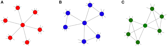
Figure 1. Network topologies, each with degree z = 6. (A) z-regular network (red) with n = 2, m = 6 and C_Δ = 0; (B) moderately clustered network (blue) with n = 3, m = 3 and C_Δ = 0.2; (C) highly clustered network (green) with n = 4, m = 2 and C_Δ = 0.4.

3. Complex Contagion Model

In this section we define our complex contagion model. First we briefly define the susceptible-infected (SI) model for comparison purposes. In the case of the continuous-time SI model (which is a simple contagion model) an infected node transmits disease to all its network neighbors at a rate β, where a neighboring node's probability of changing state from this contact is βdt in an infinitesimal time interval of length dt. A susceptible node with i infected neighbors therefore is exposed to i independent sources of infection, so the probability that the node does not become infected in a time interval dt is (1 − β dt)ⁱ, with the probability that the node does become infected being 1 − (1 − β dt)ⁱ. We define the transition rate $F_i^{SI}$ by letting the probability of infection in a small-time interval dt equal $F_i^{SI}dt$. As dt → 0 this probability becomes, βi dt, and so the transition rate for a node with i infected neighbors is

$\begin{array}{cc}{F}_i^{SI}=\beta i.& \left(2\right)\end{array}$

The transition rate scales linearly with the number i of infected neighbors, which is reasonable for a biological contagion where each possible infection event is independent of the others. However, for a social contagion a node will rarely adopt a behavior after a single exposure, it is only after several exposures that a node becomes likely to adopt [15].

As a deliberately simplified model for complex contagion we therefore propose the following transition rate function:

$\begin{array}{cc}\begin{array}{l}{F}_i^{CC}=\{\begin{array}{ll}0\hfill & \text{if }i=0,\hfill \\ 1\hfill & \text{if }i=1,\hfill \\ \beta \hfill & \text{if }i>1.\hfill \end{array}\hfill \end{array}& \left(3\right)\end{array}$

where β is the rate at which a susceptible node changes state, given multiple exposures. To model complex contagion with strong social reinforcement, for example, we can set β ≫ 1. Figure 2 compares the transition rates for SI and Complex Contagion [Equations (2) and (3), respectively] as a function of the number i of infected neighbors of a susceptible node. Considering Equation (3) and assuming β ≥ 2, if a node has multiple infected neighbors (i ≥ 2) it has an increased propensity to adopt in comparison to a node with only one infected neighbor (i = 1). In an experiment where the contagion begins with a small fraction of infected nodes the chance that a node will receive multiple exposures is much higher on a clustered network than on an random network, resulting in faster spread over clustered topologies. As we show below, this very simple representation of a complex contagion can capture the spreading behavior observed by Centola while still remaining amenable to mathematical analysis.

FIGURE 2

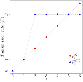
Figure 2. Comparison of transition rates, F_i for simple contagion (SI) and complex contagion (CC). Here β = 5 and i is the number of infected neighbors.

4. Clique Approximation

4.1. Clique Approximation Scheme

Many approximation schemes have been developed in order to help approximate the relationships between macroscopic observables (such as the fraction of nodes infected) and stochastic microscopic (node-level) events, such as the number of infected neighbors of each node. Such approximation schemes vary in their level of complexity, with an inherent trade-off between accuracy and complexity. There are two main approximation schemes, the mean-field (MF) and pair-approximation (PA) methods.

Briefly, the MF approximation assumes that the states of every node in the network are independent. Pair-approximation (PA) methods extend the MF approximation to incorporate information about the pair-wise correlations between susceptible nodes and their neighbors' states. For a more detailed discussion of these methods refer to Porter and Gleeson [11] and references therein. The MF and PA methods assume that the networks are locally tree-like (absence of local clustering). Violations of this assumption results in poor approximations to the true behavior of the spreading dynamics. As clustering is an integral part of the networks we consider here, we require the development of an analytical framework that can take into account both the complex contagion and the presence of clustering in clique-type networks. We will refer to this as the clique approximation (CA) scheme. Figure 3 provides a schematic of the level of local topology that each approximation scheme takes into account.

FIGURE 3

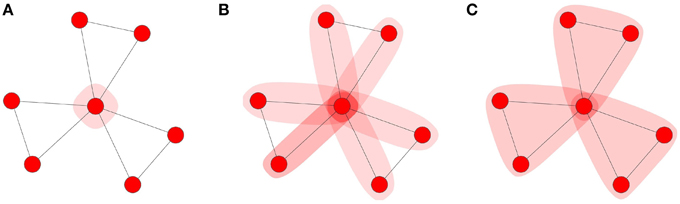
Figure 3. Approximation schemes: (A) MF, (B) PA, and (C) CA scheme. The shaded regions represents how much of the local topology is used to approximate the number of infected neighbors of an updating node.

We extend the method introduced by Hebert-Dufresne et al. [19] which they used to study SIS disease-spread dynamics (where an infected node can transition back to the susceptible state) on clique-styled networks. Our initial focus is on extending their method from simple contagions to apply it to complex contagion models such as Equation (3). In the CA scheme we track the time-dependent fraction c_i(t) of cliques that contain i infected nodes, where the transition of a clique with i infected nodes to a clique with i + 1 infected nodes is described by the time-dependent transition rate γ_i(t), as illustrated in Figure 4. Recall from Section 2 that the networks we examine are created from basic motifs where each clique had n nodes and each node is part of m cliques. Consequently, the networks are (1) z-regular (all nodes have the same degree) and (2) each node has the same local topology (refer to Figure 1 for examples).

FIGURE 4

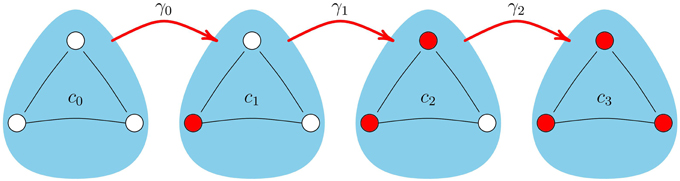
Figure 4. Transition of a clique, with n = 3, between states. Note the transition rates γ_i are time-dependent quantities, given by Equation (9).

Tracking the dynamical states of cliques, as opposed to nodes, results in a more complicated system of equations than the MF or PA methods. The added complexity is required to account for the presence of clustering in the network. We wish to calculate the fraction of infected nodes at time t, which we denote ρ(t). To create an evolution equation for ρ(t) we first calculate the rate of change of the fraction c_i(t) of cliques with i infected nodes at time t. Note the normalization condition $\sum _{i=0}^n{c}_i=1$ applies at all times t. The number of nodes that can leave a clique in state c_i−1 and enter state c_i is the total number n of nodes in that clique minus the number of nodes that are already infected at time t, i.e., n−(i−1). Similarly, the fraction of nodes that can leave a clique in state c_i and move to a clique in state c_i+1 is (n − i)c_i. Applying the relevant transition rates (γ_i−1 and γ_i, respectively) at which nodes change from one clique class to another (Figure 4) results in:

$\begin{array}{cc}\begin{array}{l}\frac{d{c}_i(t)}{dt}=(n-i+1)c_{i-1}(t){\gamma }_{i-1}(t)\hfill \\ -(n-i)c_i(t){\gamma }_i(t)\hfill \\ \text{for}i=0,1,\mathrm{...},n.\hfill \end{array}& \left(4\right)\end{array}$

(Note the explicit dependence of variables on t is henceforth omitted for convenience.) Using Equation (4) we can calculate dρ/dt by realizing that each clique with i infected nodes contributes i/n nodes to the total fraction of infected nodes:

$\begin{array}{cc}\frac{d\rho }{dt}=\frac{1}{n}{\displaystyle \sum _{i=0}^{n}i}\frac{d{c}_i}{dt}.& \left(5\right)\end{array}$

However, Equation (4) is not closed because we need to use an approximation scheme to write the transition rates γ_i in terms of the c_i(t) variables. Note that the total fraction of susceptible nodes in the network at time t is given by $1/n\sum _{i=0}^n(n-i)c_i$. We begin by calculating the probability, denoted Π_i, that at time t a chosen susceptible node is in a clique with i infected neighbors. This probability can be represented as the conditional probability Pr[i_inf|s] = Pr[(i_inf)&(s)]/Pr[s]. The numerator is the joint probability of randomly selecting a susceptible node from a clique and the clique having i infected neighbors. To calculate this we first note that the probability of selecting a clique with i infected nodes is c_i and in a c_i clique the number of susceptible nodes is (n − i). Thus, the probability of selecting a susceptible node from a c_i clique is (n−i)/n, yielding the required probability Pr[(i_inf)&(s)] = c_i(n − i)/n. The denominator (the probability of selecting a susceptible node from a clique, Pr[s]) can be obtained calculating the marginal distribution of s (i.e., by summing c_i(n − i)/n over i) yielding $\sum _{i=0}^n{c}_i(n-i)/n$. Taking the ratio of the former to the latter yields the required probability

$\begin{array}{cc}{\Pi }_i=\frac{(n-i)c_i}{{\displaystyle \sum _{j=0}^n(n-j)}{c}_j}.& \left(6\right)\end{array}$

The probability distribution Π_i can be succinctly represented as a probability generating function (PGF) (see [23] for details), which is a polynomial function defined as

$\begin{array}{cc}P(y)={\displaystyle \sum _{i=0}^n{\Pi }_i}{y}^i;& \left(7\right)\end{array}$

note that the probabilities (Π_i) can be obtained in the usual way by repeated differentiation of the PGF:

$\begin{array}{cc}{\Pi }_i=\frac{1}{i!}\frac{d^{i}P}{d{y}^i}{|}_{y=0}.& \left(8\right)\end{array}$

This PGF provides a convenient method for calculating the probabilities inside a clique. However, a susceptible node in a chosen clique also receives exposures from infected nodes in other cliques, see Figure 5. Therefore, any approximation of γ_i needs to take into account not only the infected nodes inside a clique (the green area in Figure 5), but also the probability that the susceptible node comes into contact with infected nodes in its neighboring cliques (the blue area in Figure 5). Defining ${\Pi }_{i_e}^{m-1}$ as the probability that a susceptible node in a chosen clique has i_e infected neighbors in its other m − 1 cliques, the probability distribution ${\Pi }_{i_e}^{m-1}$ has PGF [P(y)]^m−1. To approximate γ_i, we consider a clique with i infected nodes in it and look at one of the n − i susceptible nodes to calculate the probability that this node transitions to the infected state. Such a transition changes the state of the clique, moving it from the c_i class to the c_i+1 class. Consider the m − 1 other cliques that the node is part of, letting i_e be the number of infected nodes present in the neighboring cliques, then the total number of infected neighbors is i + i_e and the corresponding transition rate is F_i+ie. (Here and henceforth, we write F_i in place of $F_i^{CC}$). Of course i_e can vary from 0 to z − (n − 1), therefore to approximate γ_i we weight F_i+ie by the probability of observing i_e infected neighbors in the neighboring cliques, yielding:

$\begin{array}{cc}{\gamma }_i={\displaystyle \sum _{i_e=0}^{z-n+1}{\Pi }_{i_e}^{m-1}}{F}_{i+i_e}.& \left(9\right)\end{array}$

FIGURE 5

Figure 5. Schematic for clique approximation.

We assume that an initial fraction ρ₀ of randomly-chosen nodes are in the infected state at t = 0. The probability that a clique contains i infected nodes at t = 0 is therefore given by the binomial distribution:

$\begin{array}{cc}{c}_i(t=0)=\left(\begin{array}{c}n\\ i\end{array}\right){({\rho }_0)}^i{(1-{\rho }_0)}^{n-i},& \left(10\right)\end{array}$

which defines the initial conditions for the system given by Equation (4). With Equation (9) we can now solve Equation (4) numerically using the initial conditions (10) and thus calculate the total fraction of infected nodes at a given time for the networks of interest. In the next section we derive an early time approximation to the CA scheme to analytically find examples where quicker diffusion occurs on clustered networks than on the corresponding random network, similar to the results of Centola's experiments.

4.2. Linearization of the CA Model

In the previous section we derived the CA scheme, which captured the presence of clustering on clique-type networks. We wish to gain insight into the early spreading behavior produced by our complex contagion model (3) on the clustered networks outlined in Section 2. As previously mentioned, the CA scheme can be solved numerically using standard differential equation solvers, however it is also possible to find an approximate analytic solution to the early-time behavior. This is done by first perturbing the system (4) about a suitable fixed point and then linearizing the solution. The fixed point of interest is that corresponding to no infected nodes in the network (c₀ = 1 and c_i = 0 for i ≥ 1). We perturb this fixed point by introducing a small positive parameter ϵ such that

$\begin{array}{cc}\begin{array}{l}{c}_0=1+ϵ{\tilde{c}}_0,\hfill \\ c_i=ϵ{\tilde{c}}_i\text{for }i>0,\hfill \end{array}& \left(11\right)\end{array}$

where ${\tilde{c}}_i$ are time-dependent quantities. Applying Equation (11) to the system of Equation (4) yields the perturbed system of equations

$\begin{array}{cc}\begin{array}{l}ϵ\frac{d{\tilde{c}}_0}{dt}=-n{\gamma }_0-ϵn{\gamma }_0{\tilde{c}}_0\hfill \\ ϵ\frac{d{\tilde{c}}_1}{dt}=n{\gamma }_0+ϵn{\gamma }_0{\tilde{c}}_0-ϵ(n-1){\gamma }_1{\tilde{c}}_1\hfill \\ ϵ\frac{d{\tilde{c}}_i}{dt}=ϵ(n-i+1){\gamma }_{i-1}{\tilde{c}}_{i-1}\hfill \\ -ϵ(n-i){\gamma }_i{\tilde{c}}_i\text{ for }i>1.\hfill \end{array}& \left(12\right)\end{array}$

The γ_i's require the approximation of ${\Pi }_{i_e}^{m-1}$, the probability that a susceptible node in a chosen clique has i_e infected neighbors in the remaining m − 1 other cliques. These probabilities were built from the PGF defined by Equation (7) and applying the perturbation of Equation (11) to this results in

$\begin{array}{cc}P(y)=1+\frac{ϵ}{n}{\displaystyle \sum _{i=0}^n}((n-i){\tilde{c}}_i{y}^i-(n-i){\tilde{c}}_i)+\mathcal{O}({ϵ}^2),& \left(13\right)\end{array}$

where we are considering the asymptotic limit ϵ → 0 throughout this discussion and neglecting terms of order ϵ² and higher. We can find the PGF that corresponds to the distribution of probabilities for ${\Pi }_{i_e}^{m-1}$ by noting that

$\begin{array}{cc}{[P(y)]}^{m-1}=1+ϵ\frac{m-1}{n}{\displaystyle \sum _{i=0}^n}((n-i){\tilde{c}}_i{y}^i-(n-i){\tilde{c}}_i)+{O}({ϵ}^2).& \left(14\right)\end{array}$

Next, we use Equation (14) to retrieve the required probabilities via the usual method of differentiation (Equation (8)). Using this relationship we find the first-order approximations

$\begin{array}{cc}\begin{array}{l}{\Pi }_0^{m-1}\approx 1-ϵ\frac{(m-1)}{n}{\displaystyle \sum _{i=0}^n(n-i)}{\tilde{c}}_i,\hfill \\ {\Pi }_i^{m-1}\approx ϵ\frac{m-1}{n}(n-i){\tilde{c}}_i\text{for }i=1\text{ to }n.\end{array}& \left(15\right)\end{array}$

We are now able to approximate the γ_i's by applying Equation (15) to Equation (9) and using the fact that F₀ = 0 (i.e., nodes require an infected neighbor before they can become infected), resulting in the following

$\begin{array}{cc}\begin{array}{l}{\gamma }_i={\displaystyle \sum _{i_e=0}^n{\Pi }_{i_e}^{m-1}}{F}_{i+i_e}\hfill \\ =F_i-F_iϵ\frac{m-1}{n}{\displaystyle \sum _{i_e=0}^n(n-i_e)}{\tilde{c}}_{i_e}\hfill \\ +ϵ\frac{m-1}{n}{\displaystyle \sum _{i_e=1}^n(n-i_e)}{\tilde{c}}_{i_e}{F}_{i_e+i}+{O}({ϵ}^2).\hfill \end{array}& \left(16\right)\end{array}$

Inserting these rates into Equation (12) and noting that γ₀ is ${O}$(ϵ) while γ_i = F_i + ${O}$(ϵ) for i ≥ 1, we obtain the linearization of the CA system:

$\begin{array}{cc}\begin{array}{l}\frac{d{\tilde{c}}_0}{dt}=-(m-1){\displaystyle \sum _{i_e=1}^n(n-i_e)}{\tilde{c}}_{i_e}{F}_{i_e}+{O}(ϵ),\\ \frac{d{\tilde{c}}_1}{dt}=(m-1){\displaystyle \sum _{i_e=1}^n(n-i_e)}{\tilde{c}}_{i_e}{F}_{i_e}-(n-1)F_1{\tilde{c}}_1+{O}(ϵ),\\ \frac{d{\tilde{c}}_i}{dt}=(n-i+1)F_{i-1}{\tilde{c}}_{i-1}-(n-i)F_i{\tilde{c}}_i+{O}(ϵ)\text{for }i>1.\end{array}& \left(17\right)\end{array}$

Now we have a system of equations that describes the early spreading behavior for a general transition rate function F_i. We want to use this to find a linearized solution (ρ_l(t)) that approximates the behavior of the CA scheme. Let $\text{C}={({\tilde{c}}_0,\dots ,{\tilde{c}}_{n-1})}^T$ and further define dC/dt = f(C, t). The linearized system (17) is defined by

$\begin{array}{cc}\frac{dC}{dt}=JC,& \left(18\right)\end{array}$

where J is the n × n Jacobian matrix with element ∂f_i/∂C_j in the ith row and the jth column. Note that the ${\tilde{c}}_n$ variable does not feature in our calculation of J because it is fully determined by the relationship ${\tilde{c}}_n=1-\sum _{i=0}^{n-1}{\tilde{c}}_i$. The general solution of systems like (18) typically can be written as

$\begin{array}{cc}C(t)={\displaystyle \sum _{j=0}^{n-1}{\xi }_j}{e}^{{\lambda }_{j}t}{u}_j,& \left(19\right)\end{array}$

where ξ_j is a constant, λ_j is the eigenvalue and u_j is the corresponding eigenvector of J [24]. The constants ξ_j can be calculated by using the initial conditions $\text{C}(t=0)=\sum _{j=0}^n{\xi }_j{\text{u}}_j$ (refer to Equation (10) for initial conditions for the system). The fixed point that we considered was c₀ = 1 and c_i = 0 for i > 0, where there were no infected nodes on the network. Our linearized solution is therefore valid for small perturbations from this, i.e., when the initial fraction of infected nodes is small (ρ(t) is small and ${O}({\rho }_0^2)$ terms are negligible). The linearized approximation to the total fraction of infected nodes at time t is given by

$\begin{array}{cc}\rho (t)\approx {\rho }_l(t)=\frac{1}{n}{\displaystyle \sum _{i=0}^{n}i}{\tilde{c}}_i(t).& \left(20\right)\end{array}$

This formulation now allows us to examine the early-time spreading behavior that is produced by our complex contagion model (and see Appendix B for a simple worked example). It is also possible to find the level of social reinforcement β for which a clustered network will propagate a complex contagion faster than a random network. The largest eigenvalue of the Jacobian matrix (which we denote λ_max) appearing in the linearization Equation (19) provides the largest contribution to the early-time growth of Equation (20), and so to ρ(t). Thus, by comparing the λ_max value for each network for a given β and noting which network has the larger value, we can infer the case where the complex contagion will diffuse faster, at least at early times. This will be used in the following section in conjunction with the full CA scheme and the linearized solution to examine the complex contagion model on networks with various levels of clustering.

5. Results

In Section 4.1 we described the clique approximation (CA) scheme that we use to account for the presence of clustering in clique-type networks for monotone binary-state dynamics. We also linearized the CA scheme to approximate the early-time spreading behavior (Section 4.2). In this section, we compare the accuracy of the full CA scheme and the linearized approximation to Monte Carlo (MC) simulations of the complex contagion model given by Equation (3) (for details on simulations please refer to Appendix C). This allows us to establish the accuracy of both the CA scheme and its linearized approximation across clique-type networks and varying level of social reinforcement (as parameterized by β).

Recall that we consider three z-regular network topologies with degree 6 (refer back to Figure 1). First, a random network (n = 2 and m = 6), which has the lowest density of triangles (C_Δ = 0), then a moderately clustered network where each clique has three nodes and each node is part of three cliques (C_Δ = 0.2), and lastly, a highly clustered network where each clique has four nodes and each node is a part of 2 cliques (C_Δ = 0.4). Figure 6 presents the results across the three topologies that we consider and for two values of β. The CA method clearly provides a highly accurate approximation to ρ(t) across the three network topologies. The linearized approximation of the CA scheme also provides accurate approximations for the early-time growth of ρ(t). However, once the fraction of infected nodes becomes large during the later stages of spreading the approximation begins to break down.

FIGURE 6

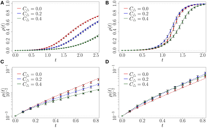
Figure 6. Fraction ρ(t) of infected nodes from CA and linearized solution, compared with Monte Carlo simulations (symbols), on random (red), moderately clustered (blue), and highly clustered (green) networks. (A) β = 1, CA scheme; (B) β = 6, CA scheme; (C) β = 1, linearized; (D) β = 6, linearized. Symbols represent the mean of 10 Monte Carlo realizations (the error bars indicate one standard deviation above and below the mean), solid lines represent the CA results, and dashed lines the linearized approximation. Note that the y-axis of (C,D) are logarithmic. The initial fraction of infected is ${\rho }_0=10^{-3}$, simulated network sizes are N = 10⁵, using step size dt = 10⁻³.

Now we examine the spreading behavior that our complex contagion model $F_i^{CC}$ produces on clustered networks. In the definition of $F_i^{CC}$ the parameter β is the rate at which a susceptible node will become infected if more than one of its neighbors is infected. As β increases we expect the infection to spread faster on the two clustered networks than on the random network (at least at early times) because of the existence of reinforcement signals from triangles.

For comparison, we consider β = 1, meaning that a susceptible node with one infected neighbor has the same infection rate as a susceptible node with multiple infected neighbors. From Figures 6A,C we see that in this case the behavior spreads fastest on the random (C_Δ = 0) network, because the random network allows the maximum number of unique exposures from newly infected nodes.

However, for larger values of β it becomes more advantageous for early-stage spreading to have a non-zero density of triangles than a tree-like structure in the local topology. By increasing β to 6 we find this is the case (see Figure 6D). Note that at early times (before t = 1) the random network consistently infects a lower fraction of the population than the clustered networks; we analyze this phenomenon further below.

Empirical observations of spreading behavior on networks shows that typically only a small fraction of the total network ever adopts a behavior. Centola [15] observed that the average percentage of the network that adopted was 38 and 53% for the random and clustered networks respectively. The networks used in his experiments were relatively small, with N ≤ 144 nodes. If our complex contagion model is reflective of the spreading behavior in real life contagions we should observe the same behavior for small ρ(t) which corresponds to the early-time behavior (which we consider in Figure 8). Before we examine this in detail we calculate the critical reinforcement levels for which we expect clustered networks to produce faster early time spreading than the random network (at least in the limit of very large network size, N → ∞, for which our approximations are valid).

As mentioned in Section 4.2, by finding the network topology with the largest λ_max for a given β we can identify which network will produce the fastest diffusion of an early-stage complex contagion. For the random network topology (C_Δ = 0) the largest eigenvalue is λ_max = 4. For the moderately clustered network topologies the largest eigenvalue is ${\lambda }_{max}=1/2(2-\beta +\sqrt{4+20\beta +{\beta }^2})$, while the highly clustered network topology has largest eigenvalue ${\lambda }_{max}=1/2(-\beta +\sqrt{\beta }\sqrt{24+\beta })$. By plotting how these vary with β we can identify the level of social reinforcement required to produce faster spreading on the clustered networks than on the random network at early time. From Figure 7 we note that for β > 4 (respectively, β > 8) the moderately (highly) clustered network should produce faster diffusion than the random network. The main limitation of the predicted critical β's is that the exponential growth rate λ_max must dominate in Equation (19) over a sufficient range for its contributions to become pronounced. To obtain this behavior ρ₀ must be very small. This ensures that the initial transient behavior (the contributions from the other eigenvalues) dies off quickly and the exponential growth at rate λ_max dominates. Therefore, in Figure 8 we show the predicted fraction of infected nodes from the full CA model at early stages for a very small fraction of infected nodes, ${\rho }_0=10^{-8}$, which would correspond to a very large network.

FIGURE 7

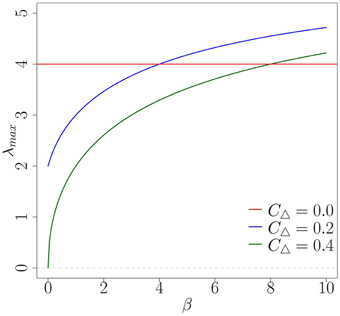
Figure 7. Comparison of λ_max for varying β on the three network topologies. The largest eigenvalues for the moderately clustered network (blue) and the highly clustered network (green) intercept the random case (red) at β = 4 and β = 8, respectively.

FIGURE 8

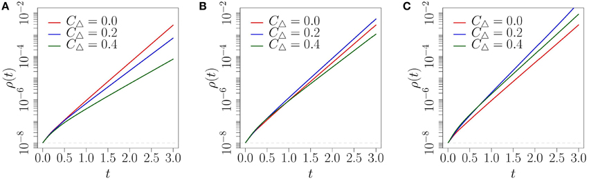
Figure 8. Fraction ρ(t) of infected nodes on three network topologies, using the CA scheme: (A) β = 2; (B) β = 5; (C) β = 10. Note that the y-axis is logarithmic and ${\rho }_0=10^{-8}$.

Similar to what we observed in Figure 6, the level of social reinforcement dictates how fast the diffusion spreads on each network at early times in Figure 8. We also observe that the order of the networks that provide the fastest diffusion is well reflected by the comparison of each network's λ_max illustrated in Figure 7. More specifically, in Figure 8A where β = 2, we see that the level of social reinforcement is not high enough to cause faster spreading on the clustered networks than on the corresponding random network. Increasing β to 5 we observe faster spreading on the moderately clustered network than on the random network, with the highly clustered network producing the slowest diffusion (see Figure 8B). Increasing β further to 10 we observe faster spreading of both clustered networks over the random network (Figure 8C), again in accordance with what is expected from Figure 7. Although the critical levels of social reinforcement predicted in Figure 7 are accurate for ρ₀ ≪ 1, qualitatively similar behavior is produced for larger values of ρ₀ (refer to Figure 6), but with stronger influence of initial transients.

Finally, we show for completeness that our complex contagion model can produce faster spreading on a hexagonal lattice compared with a random network, which mimics Centola's experimental setup (see Appendix A for details). The topology of the hexagonal lattice is illustrated in Figure 10A, and it has clustering coefficient of 0.4. We simulate the complex contagion on this network using the Monte Carlo method on large networks (N = 10⁵) with the hexagonal lattice structure.

The results of the simulations are compared to the expected diffusion on a random and highly clustered network of the same degree (z = 6) using the CA method (see Figure 9). We find similar results to those noted in the analysis of the clique-type networks. For low levels of social reinforcement (β ≤ 3) the random network provides the fastest spreading (see Figures 9A,B). However, when β is increased to 4 we observe faster diffusion on the hexagonal lattice and the highly clustered network than on the corresponding random network (see Figure 9C). Both the hexagonal lattice and the highly clustered network appear to have roughly the same critical level of social reinforcement for this initial fraction of infected nodes (${\rho }_0=10^{-3}$). By increasing β further to 10 (see Figure 9D) we find that the hexagonal lattice provides the fastest diffusion at early time.This is interesting as both the highly clustered network and the hexagonal lattice have the same clustering coefficient of C_Δ = 0.4. This is explained by the difference in structure between the hexagonal lattice and the highly clustered network. The hexagonal lattice has a higher density of cycles of length greater than 3. The highly clustered network on the other hand has a lower density of cycles of length greater than 3 as each node is randomly connected to each clique. This results in faster spreading on the hexagonal lattice at early time than on the highly clustered network due to the increased chance of a susceptible node receiving multiple exposures from infected nodes. This qualitatively reproduces the pattern of spreading behavior observed by Centola, where for a sufficient level of social reinforcement it is possible to produce faster spreading on clustered networks than a random network of the same degree. In the next section we conclude the paper with a summary, some comments on the results and provide possible directions for future research.

FIGURE 9

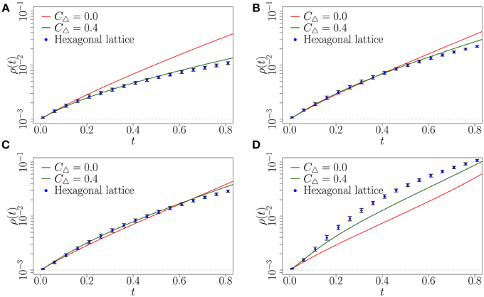
Figure 9. Fraction ρ(t) of infected nodes on random network (solid red line), highly clustered clique-type network (solid green line) and hexagonal lattice (blue points). Solid lines represent the results from the CA method. Symbols represent the mean of 10 Monte Carlo realizations (the error bars indicate one standard deviation above and below the mean). (A) β = 1; (B) β = 3; (C) β = 4; (D) β = 10. Parameters ρ₀, N and dt are as in Figure 6.

6. Conclusion

In this paper we aimed to model—in an analytically tractable fashion—the spreading of behaviors such as the adoption of new innovations. Such spreading processes are influenced by the social networks that connect people. Centola performed an experiment where he tracked the diffusion of such behavior (the use of a health forum) across artificially created networks [15]. These networks allowed him to control the level of clustering (density of cycles of length three) in the local topology and to isolate its effect on how the behavior diffused (refer to Figure 10). He observed that nodes that received multiple reinforcing signals had a higher propensity to adopt compared to those that only received one signal, which was much more beneficial to the spreading of the contagion on the clustered networks. This resulted in the contagion spreading farther and faster on the clustered-lattices than on the corresponding random networks.

FIGURE 10

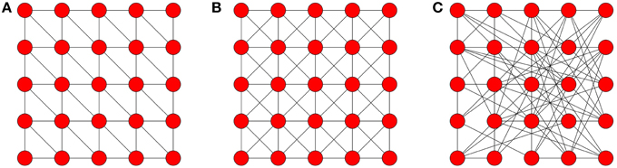
Figure 10. Network topologies. Note that Centola used networks of sizes 98, 128, and 144. These networks are wrapped around a torus to maintain the degree of each node. (A) hexagonal neighborhood; (B) Moore lattice; (C) random graph.

Our goal was to find a suitably simple characterization for complex contagion that remained amenable to analysis. We proposed modeling the complex contagion using monotone binary-state dynamics with the transition rate function defined by $F_i^{CC}$ (see Section 3). Each node is either susceptible (has not yet adopted) or infected (adopted). This simple characterization proved to be quite effective in enabling us to obtain analytical insight. We compared the spreading behavior produced by the complex contagion model across three topologies with varying levels of clustering (see Figure 1 for the topologies and Figure 6 for results). By varying the propensity for a node to become infected given multiple infected neighbors we were able to produce faster spreading on clustered networks then on the random network, which is qualitatively similar behavior to that observed by Centola (Figure 6B). We also showed, via simulation, that our complex contagion model could produce similar spreading behavior between a hexagonal lattice and comparable random network as the previously mentioned analytic results for the clique-type networks (see Figure 9).

None of these results could have been obtained without tackling the problem of approximating monotone binary-state dynamics on clustered networks. As described in Section 4.1, standard approximation schemes (mean-field and pair approximation) perform poorly in the presence of clustering. They are heavily dependent on the assumption that the network is locally tree-like (that is no cycles of length three in the network). However, the use of clustered networks is crucial to the examination of the complex contagion model, as the presence of triangles are central to the social reinforcement mechanism that we wished to examine. This necessitated the development of the CA method which accurately accounted for the effects of clustering in the local topology of the clique-based networks we examined (see Section 4 for details). The CA method proved to be highly accurate for these types of topologies. A linearized approximation to the early-time spreading behavior of the complex contagion model was obtained. Using this we were able to calculate critical levels of social reinforcement required for the contagion to spread faster on clustered networks than on the corresponding random network (refer to Figure 7).

The characterization of a complex contagion spreading process by a single-parameter function in Equation (3) provided a suitable balance between simplicity and realistic behavior. However, the approximation scheme we develop is applicable to any F_i function, and so more realistic models can easily be examined in this framework. Further examination of more realistic characterization of complex contagions should also be developed, for example including a time-decay in the memory of each node. It is reasonable to assume that the true mechanism that governs complex contagion depends on the interplay between the strength of social reinforcement and also temporal effects, such as the timing between exposures.

Author Contributions

JG and PF designed the research and developed the approximation schemes; DOS and GOK performed the calculations and numerical simulations; DOS led the writing of the paper.

Conflict of Interest Statement

The authors declare that the research was conducted in the absence of any commercial or financial relationships that could be construed as a potential conflict of interest.

Acknowledgments

This work was partly funded by Science Foundation Ireland (awards 11/PI/1026 and 12/IA/I683), the Irish Research Council (award GOIPG/2014/887) and by the European Commission through FET-Proactive project PLEXMATH (FP7-ICT-2011-8; grant number 317614).

References

1. Newman MEJ. Properties of highly clustered networks. Phys Rev E (2003) 68:026121. doi: 10.1103/PhysRevE.68.026121

CrossRef Full Text | Google Scholar

2. Ugander J, Backstrom L, Marlow C, Kleinberg J. Structural diversity in social contagion. Proc Natl Acad Sci USA. (2012) 109:5962–6. doi: 10.1073/pnas.1116502109

CrossRef Full Text | Google Scholar

3. Broder A, Kumar R, Maghoul F, Raghavan P, Rajagopalan S, Stata R, et al. Graph structure in the web. Comput Netw. (2000) 33:309–20. doi: 10.1016/S1389-1286(00)00083-9

CrossRef Full Text

4. Maslov S, Sneppen K. Specificity and stability in topology of protein networks. Science (2002) 296:910–3. doi: 10.1126/science.1065103

PubMed Abstract | CrossRef Full Text | Google Scholar

5. Aral S, Muchnik L, Sundararajan A. Distinguishing influence-based contagion from homophily-driven diffusion in dynamic networks. Proc Natl Acad Sci USA. (2009) 106:21544–9. doi: 10.1073/pnas.0908800106

CrossRef Full Text | Google Scholar

6. Baños RA, Borge-Holthoefer J, Moreno Y. The role of hidden influentials in the diffusion of online information cascades. EPJ Data Sci. (2013) 2:1–16. doi: 10.1140/epjds18

CrossRef Full Text | Google Scholar

7. Nematzadeh A, Ferrara E, Flammini A, Ahn YY. Optimal network modularity for information diffusion. Phys Rev Lett. (2014) 113:088701. doi: 10.1103/PhysRevLett.113.088701

PubMed Abstract | CrossRef Full Text | Google Scholar

8. Borge-Holthoefer J, Baños RA, González-Bailón S, Moreno Y. Cascading behaviour in complex socio-technical networks. J Complex Netw. (2013) 1:3–24. doi: 10.1093/comnet/cnt006

CrossRef Full Text | Google Scholar

9. Centola D, Macy M. Complex contagions and the weakness of long ties. Am J Sociol. (2007) 113:702–34. doi: 10.1086/521848

CrossRef Full Text | Google Scholar

10. Kitsak M, Gallos LK, Havlin S, Liljeros F, Muchnik L, Stanley HE, et al. Identification of influential spreaders in complex networks. Nat Phys. (2010) 6:888–93. doi: 10.1038/nphys1746

PubMed Abstract | CrossRef Full Text

11. Porter MA, Gleeson JP. Dynamical systems on networks: a tutorial (2014). arXiv preprint arXiv:1403.7663.

Google Scholar

12. Newman ME, Park J. Why social networks are different from other types of networks. Phys Rev E (2003) 68:036122. doi: 10.1103/PhysRevE.68.036122

PubMed Abstract | CrossRef Full Text | Google Scholar

13. Watts DJ, Strogatz SH. Collective dynamics of small-worldnetworks. Nature (1998) 393:440–2. doi: 10.1038/30918

PubMed Abstract | CrossRef Full Text | Google Scholar

14. Shirley MD, Rushton SP. The impacts of network topology on disease spread. Ecol Complex. (2005) 2:287–99. doi: 10.1016/j.ecocom.2005.04.005

CrossRef Full Text | Google Scholar

15. Centola D. The spread of behavior in an online social network experiment. Science (2010) 329:1194–7. doi: 10.1126/science.1185231

PubMed Abstract | CrossRef Full Text | Google Scholar

16. Lü L, Chen DB, Zhou T. The small world yields the most effective information spreading. N J Phys. (2011) 13:123005. doi: 10.1088/1367-2630/13/12/123005

CrossRef Full Text | Google Scholar

17. Pastor-Satorras R, Vespignani A. Epidemic spreading in scale-free networks. Phys Rev Lett. (2001) 86:3200. doi: 10.1103/PhysRevLett.86.3200

PubMed Abstract | CrossRef Full Text | Google Scholar

18. Gleeson JP. Binary-state dynamics on complex networks: pair approximation and beyond. Phys Rev X (2013) 3:021004. doi: 10.1103/PhysRevX.3.021004

CrossRef Full Text | Google Scholar

19. Hébert-Dufresne L, Noël PA, Marceau V, Allard A, Dubé LJ. Propagation dynamics on networks featuring complex topologies. Phys Rev E (2010) 82:036115. doi: 10.1103/PhysRevE.82.036115

PubMed Abstract | CrossRef Full Text | Google Scholar

20. Newman MEJ. Networks: An Introduction. New York, NY: Oxford University Press (2010). doi: 10.1093/acprof:oso/9780199206650.001.0001

CrossRef Full Text | Google Scholar

21. Newman ME. The structure and function of complex networks. SIAM Rev. (2003) 45:167–256. doi: 10.1137/S003614450342480

CrossRef Full Text | Google Scholar

22. Miller JC. Percolation and epidemics in random clustered networks. Phys Rev E (2009) 80:020901. doi: 10.1103/PhysRevE.80.020901

PubMed Abstract | CrossRef Full Text | Google Scholar

23. Johnson NL, Kemp AW, Kotz S. Univariate Discrete Distributions. Vol. 444. Hoboken, NJ: John Wiley & Sons (2005). doi: 10.1002/0471715816

CrossRef Full Text | Google Scholar

24. Drazin PG. Nonlinear Systems. Vol. 10. Cambridge, UK: Cambridge University Press (1992).

Google Scholar

Appendix

A. Centola's Experimental Design

Centola investigated the effects of network structure on the spread of behavior through artificially structured online communities. These networks were carefully created to allows for direct comparison between random graphs (low C_Δ) and clustered lattices (high C_Δ).

In his experiment each network represents the connections of an artificially created on-line health community. Each participant created an anonymous on-line profile, they were then linked to other participants according to a predefined topology (see Figure 10 for examples). Each participant could not communicate with each other directly but were informed of their activities. Participants made decisions on whether or not to adopt a behavior based on their neighbors' activity, in this case the registration to a health forum. The diffusion process was initiated by selecting a random seed node, which signaled (via an automatically sent email) its neighbors, encouraging them to register for the forum. Every time a participant adopted the behavior (registered to the forum), messages were sent to his network neighbors. As the number of nearest neighbors that registered increased, the participant received more signals. Several trials were conducted on two different clustered topologies and two unclustered topologies.

The Hexagonal lattice and Moore lattice corresponded to the clustered topologies used, each having a fixed degree of six and eight for all nodes with a clustering coefficient of 0.4 and 0.43 (see Figures 10A,B), respectively. Each clustered topology was then compared to a random network, where each node has the same degree but the links were randomly assigned, as illustrated in Figure 10C (a random network with fixed degree). Random graphs have the lowest clustering coefficients of all the graphs that Centola used.

B. Linearization - Worked Examples

In this section we provide a simple example of the linearized approximation of the CA scheme described in Section 4.2. The spreading dynamics that we will approximate is the behavior of our complex contagion model defined in Section 3 on a z-regular random network (zero clustering case). Recall that random networks can be described by n = 2 and m = 6, where each node in the network has degree six (see Figure 1). Applying these values to the linearized system of Equation (17) we have

$\begin{array}{cc}\begin{array}{l}\frac{d{\tilde{c}}_0}{dt}=-5{\displaystyle \sum _{i_e=1}^2(2-i_e)}{\tilde{c}}_{i_e}{F}_{i_e}^{CC}+{O}(ϵ),\hfill \\ \frac{d{\tilde{c}}_1}{dt}=5{\displaystyle \sum _{i_e=1}^2(2-i_e)}{\tilde{c}}_{i_e}{F}_{i_e}^{CC}-(2-1)F_1^{CC}{\tilde{c}}_1+{O}(ϵ).\hfill \end{array}& \left(\text{A}1\right)\end{array}$

Recall that we do not require the ${\tilde{c}}_n$ variable as it is fully determined by the other ${\tilde{c}}_i$ variables. The next stage in this approximation is to compute the Jacobain matrix for this system:

$\begin{array}{cc}J=\left(\begin{array}{cc}0& -5\\ 0& 4\end{array}\right).& \left(\text{A}2\right)\end{array}$

Matrix (A2) has eigenvalues λ₁ = 4 and λ₂ = 0, each with associated eigenvectors ${\text{u}}_1={(-5,4)}^T$ and ${\text{u}}_2={(1,0)}^T$, respectively. Applying these to Equation (19), we obtain

$\begin{array}{cc}C(t)={\xi }_1{e}^{{\lambda }_{1}t}{u}_1+{\xi }_2{e}^{{\lambda }_{2}t}{u}_2.& \left(\text{A}3\right)\end{array}$

The constants (ξ₁ and ξ₂) can be easily obtained by noting that $\text{C}(t=0)=\sum _{j=0}^n{\xi }_j{\text{u}}_j$ must equal the initial conditions of Equation (10). We ignore ${O}({\rho }_0^2)$ terms, which yields ξ₁ = ρ₀/2 and ξ₂ = 1 − ρ₀/2. With these constants we are able to calculate the linearized approximation to the fraction of infected nodes on a z-regular random network given by Equation (20) as

$\begin{array}{cc}{\rho }_l(t)=\frac{3}{2}{\rho }_0{e}^{4t}-\frac{{\rho }_0}{2}.& \left(\text{A}4\right)\end{array}$

Notably, in this simple example we find that β ($F_i^{CC}$ for i ≥ 2) does not feature in the result, this is a direct consequence of the assumption that the local topology generated by n = 2 and m = 6 is locally tree-like. Equation (A4) provides an accurate approximation to the early-time spreading behavior of a complex contagion on a tree-like network of degree 6, provided that the initial fraction of infected nodes is small (see Figure 6).

C. Simulation Method

To simulate monotone binary-state dynamics we use Monte Carlo (MC) simulation. To represent the network in the simulations we use an adjacency matrix A, where

$\begin{array}{cc}\begin{array}{l}{A}_{ij}=\{\begin{array}{ll}1\hfill & \text{if there is a link between nodes }i\text{ and }j,\hfill \\ 0\hfill & \text{otherwise, }\hfill \end{array}\hfill \end{array}& \left(\text{A}5\right)\end{array}$

defines an N × N matrix, where N is the number of nodes. Given this matrix we know the connections between nodes. We track the state of each node using the vector v (a N × 1 vector). The element v_i is 0 if the node is susceptible and 1 if infected. To initialize the simulation we randomly assign a fraction ρ₀ of nodes to the infected state at time 0. We wish to simulate the dynamics for the complex contagion model defined in Section 3 by Equation (3). The transition rates in these models depend on the number of infected neighbors of a node. Let η be an N × 1 dimensional vector where η_i is the number of infected neighbors of node i. The vector of η_i values can be easily calculated using the matrix multiplication

$\begin{array}{cc}\eta =Av.& \left(\text{A}6\right)\end{array}$

The probability that node i will change state is given by p = F_ηidt, where F_ηi is the transition rate for node i (which has η_i infected neighbors). This gives the update rule for the state of node i, where v_i = 1 if p > u, for u drawn from a uniform distribution on [0, 1]. The fraction of infected nodes is then updated ($\rho (t+dt)=\frac{1}{N}\sum \text{v}$) and time, t, is advanced by dt. These steps are repeated until either ρ(t) = 1 or until a maximum time is reached (t_max). This process yields one realization of the dynamics, it is repeated M times (the number of MC realizations) and the ensemble-average fraction of infected nodes is calculated to approximate the expected behavior of the dynamics. The parameters used for simulations are as follows unless otherwise stated: N = 10⁵, ρ₀ = 10⁻³, t_max = 3, dt = 10⁻³ and M = 10.