Temporal pattern of online communication spike trains in spreading a scientific rumor: how often, who interacts with whom?

1. Introduction

In recent years, online social media (OSM) have become a major communication channel, allowing users to share information in their social and professional circles, to discover relevant information pre-filtered by other users, and to chat with their acquaintances. In addition to their practical use for individuals, OSM have the advantage of generating a rich data set on collective social dynamics, as social relations among individuals, temporal properties of their interactions, and their contents are automatically stored. The study of these digital footprints has led to the emergence of computational social science, allowing to quantify at large-scales our political ideas and preferences [1], to discover roles in social networks [2, 3], to predict our health [4] and personality [5], and to determine external effects on online behavior [6]. Importantly, in OSM, users are at the same time both actors and receivers and therefore the amplification of a trend originates from the interplay between influencing [7, 8] and being influenced [9–13].

A crucial aspect of OSM and more generally of human behavior is the underlying complex dynamics [14–17]. The time series of user activities, e.g., posting a tweet and replying to a message, are quite distinct from uncorrelated (Poisson random) dynamics in the presence of burstiness [18–20], temporal correlations [6, 21, 22], and non-stationarity of human daily rhythm [23, 24], which has significant implications. Diffusion on a temporal network cannot be accurately described by models on static networks and consequently the process presents non-Markovian features with strong influence on the time required to explore the system [25, 26]. Furthermore, the dynamics drives a strong heterogeneity observed in user activity [27, 28] and user/content popularity [29–31]. Specifically, in Twitter, the heterogeneity in popularity has been observed and quantified in different ways by the size of retweet cascades, i.e., users re-transfer messages to their own followers with or without modifying them [32–36] or by the number of mentions of a user name, identified by the symbol @, in other people's tweets [37].

In this paper, we focus on the dynamics of social interactions taking place when diffusing rumors about the discovery of the Higgs boson on July 2012 in Twitter [38]. Our main goal is to find connections between the statistical properties of user time series established on the same subject, e.g., the announcement of the discovery of the Higgs boson, and their activity and popularity. To this end, we analyze tweets including social interactions, such as retweets of a message (RT), mentions of a user name (@), and replies to a message (RE). For each type of the interactions, a user can either play an active, e.g., retweeting, or a passive, e.g., being retweeted, role. Therefore, we characterize each user by 8 time series: one active and one passive time series for each of the 3 types of interaction as well as for the aggregation of all interactions, as illustrated in Figure 1. Active time series are denoted as WHO and passive time series are defined by WHOM. We then investigate whether the statistical properties of each signal is a good predictor for the activity and popularity of a user.

FIGURE 1

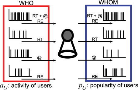
Figure 1. Illustration of communications in Twitter. The sketch summarizes the two positions of each user, e.g., active (who) and passive (whom). Who interacts in time with any other whom by retweeting (RT) the messages and mentioning (@) the user names of whom in a message and replying (RE) to the messages from whom. Quantifying temporal patterns in time series of who with various ranges of the activity of users a_U and of whom by increasing the popularity of users p_U is the main scope of this paper.

The following sections are organized as follows. In Section 2, we describe the data set and provide basic statistical properties of who and whom time series. In Section 3, we introduce a technique dedicated to the analysis of non-stationary time series, so-called local variation, originally established for neuron spike trains [39–42] and recently applied to hashtag spike trains in Twitter [43, 44]. In Section 4, we search for statistical relations between local variation and measures of popularity of a user. Finally, Section 5 summarizes the key results and raises open questions.

2. Activity and Popularity of Users

Our aim is to examine the dynamics of user communications in Twitter. We investigate how frequently users talk to each other on a certain topic, e.g., the discovery of the Higgs boson, and identify how complex dynamic patterns of the communications evolve in time. To this end, we focus on the three different types of interaction between users, retweet (RT), mention (@), and reply (RE). Twitter users can adopt a tweet of someone and use it again in their own tweet by RT or contact to other users directly by typing user names in a message called @ or simply RE to any tweets, e.g., regular tweets, retweets, and tweets/retweets including @s. Typically, @s and REs are associated to personal interactions between users, whereas RTs are responsible for large-scale information diffusion in the social network and for the emergence of cascades. Here, we count all types of interaction as a part of complex information diffusion in the network.

Interactions in Twitter are performed between at least two users (for instance, a user can mention several other users in a single tweet). Each action is directed and characterized by its timestamp. The users performing the action play active roles (who users), the users receiving their attention play a passive role (whom users), and each user can appear in both active and passive roles described in Figure 1. Therefore, we construct active and passive RT, @, and RE spike trains for each user.

2.1. Data Set

As a test bed, we consider the publicly available Higgs Twitter data set [38, 45], first collected to track the spread of the rumor on the discovery of the Higgs boson via RT, @, or RE. The data set is composed of tweets containing one of the following keywords or hashtags related to the discovery of the Higgs boson, “lhc,” “cern,” “boson,” and “higgs.” The start date is the 1st July 2012, 00:00 a.m. and the final date is the 7th July 2012, 11:59 p.m., which covers the announcement date of the discovery, the 4th July 2012, 08:00 a.m. All dates and timestamps in the data are converted to the Greenwich mean time. Detailed information on the data collection procedure and basic statistics can be found in Domenico et al. [38].

In total, the data is composed of 456,631 users (nodes) and 563,069 interactions (edges). Among those, we detect 354,930 RT, 171,237 @, and 36,902 RE, which shows that RT is more popular than the other communication channels. For RT interactions, we find 228,560 users join in who, in contrast, only 41,400 users appear in whom. These numbers are smaller for @, e.g., 102,802 who and 31,477 whom, and even smaller for RE, with 27,227 who and 18,578 whom. In each case, whom is much lower than who, as expected because a small number of users tend to attract a large fraction of attention in both friendship [46, 47] and online social [48–52] networks. This observation is confirmed in Figure 2, where we present Zipf plots associated to each interaction, clearly showing a strong heterogeneity in the system. For who, the frequency of the user communication f_U ranks how active users are and measures the activity of users a_U, on the other hand, for whom, f_U quantifies how often the users or their tweets are addressed and so gives the popularity of users p_U.

FIGURE 2

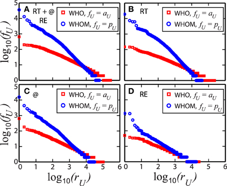
Figure 2. How often users in who pool communicate with users appear in whom. Zipf plots describe heterogeneities of users in the types of Twitter interaction, e.g., (A) all of retweet, RT, mention, @, and reply, RE, (B) only RT, (C) only @, and finally (D) only RE. The frequency of the communication f_U is measured in two-fold: The activity of who (red squares) a_U and the popularity of whom (blue circles) p_U. The x−axis ranks the users r_U from high f_U to low values. Each plot indicates that who more likely contacts to someone, as observed in the smoother decays, however only few users in whom are addressed and become popular in these communications.

3. Local Variation of Who and Whom

3.1. Communication Spike Trains

Evaluating each directed interaction (RT, @, and RE) of the users in the pool of who with any users in the whom class, as sketched in Figure 1, we extract salient temporal patterns of the user communication time series. We don't check whether the whom participates in the conversation in a later stage and only construct independent time series of the individual who and whom. The elements of the time series are the timestamps of the data [38, 45] providing us the exact time in second of the interaction and the user name or ID of the corresponding who and whom. Ordering the timestamps from the earliest to the latest, we generate spike trains carrying full story of the communication of each user. The resultant user communication spike trains are grouped in eight: For each who and whom, the spike trains of all interactions together (i) and the spike trains of filtered timestamps of RT (ii), @ (iii), and RE (iv).

3.2. Local Variation

A standard way of investigating the dynamics of human communication is to examine the statistics of the inter-event spike intervals such as its probability distribution [14], short-range memory coefficient and burstiness parameter [15] or Fano factor. However, recent works have showed that further detail analysis is required to resolve temporal correlations [31, 32], bursts [19–22], and cascading [53] driven by circadian rhythm [23, 24], complex decision-making of individuals [3, 27, 54], and external factors [6] such as the announcement of discoveries, as considered in the current data [38].

To uncover the dynamics of the communication spike trains elaborately, we apply the local variation L_V originally defined to characterize non-stationary neuron spike trains [39–42] and very recently has been used to analyze hashtag spike trains [43, 44]. Unlike the memory coefficient and burstiness parameter [15], L_V provides a local temporal measurement, e.g., at τ_i of a successive time sequence of a spike train …, τ_i−1, τ_i, τ_i+1, …, and so compares temporal variations with their local rates [41]

$\begin{array}{ll}{L}_V=\frac{3}{N-2}{\displaystyle \sum _{i=2}^{N-1}}{\left(\frac{({\tau }_{i+1}-{\tau }_i)-({\tau }_i-{\tau }_{i-1})}{({\tau }_{i+1}-{\tau }_i)+({\tau }_i-{\tau }_{i-1})}\right)}^2& (1)\end{array}$

where N is the total number of spikes. Equation (1) also takes the form [41]

$\begin{array}{ll}{L}_V=\frac{3}{N-2}{\displaystyle \sum _{i=2}^{N-1}}{\left(\frac{\Delta {\tau }_{i+1}-\Delta {\tau }_i}{\Delta {\tau }_{i+1}+\Delta {\tau }_i}\right)}^2& (2)\end{array}$

Here, Δτ_i+1 = τ_i+1−τ_i quantifies the forward delays and Δτ_i = τ_i−τ_i−1 represents the backward waiting times for an event at τ_i. Importantly, the denominator normalizes the quantity such as to account for local variations of the rate at which events take place. By definition, L_V takes values in the interval (0:3) [43]. It has been shown that helps at classifying dynamical patterns successfully [39, 40, 42–44]. Following the analysis of Gamma processes [39, 40, 43] conventional in neuron spike analysis [42], it is known that L_V = 1 for temporarily uncorrelated (Poisson random) irregular spike trains, and that higher values are associated to a burstiness of the spike trains. In contrast, smaller values indicate a higher regularity of the time series.

We now perform an analysis of L_V on the user communication spike trains. Equation (2) is performed through the spike trains with removing multiple spikes taking place within 1 s. Such events are rare and their impact on the value of L_V has been shown to be limited [43]. Figure 3 describes the distribution of L_V, P(L_V) of full spike trains all together with RT, @, and RE for the who (a, b) and whom (c, d). Grouping L_V based on the frequency f_U, e.g., the activity of the who a_U and the popularity of the whom p_U, we examine the temporal patterns of the trains in different classes of a_U and p_U. For the real data in (a, c), in Figure 3A, L_V is always larger than 1 in any values of a_U, suggesting that all users playing a role in who contact to the whom in bursty communications. However, in Figure 3C, we observe distinct behavior of the whom users and bursts present only for low p_U. By increasing p_U, L_V ≈ 1 indicating that there is no temporal correlation among the who referring the whom and L_V is slightly smaller than 1 for the most popular users, indicating a tendency toward regularity in the time series, as also observed for the hashtag spike trains [43]. These observations are significantly different for artificial spike trains constructed by randomly permuting the real full spike train and so expected to generate non-stationary Poisson processes. Therefore, all distributions are centered around 1 in this case, independently of a_U and p_U, as shown in Figures 3B,D. The randomization and obtaining a null set follow the same procedure explained in detail in Sanli and Lambiotte [43].

FIGURE 3

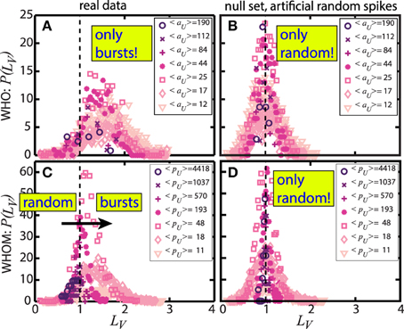
Figure 3. Probability density function of the local variation L_V, P(L_V) of who (A,B) and whom (C,D) users in various ranges of the two communication frequencies, e.g., a_U and p_U. (A,C) describe the results of the real data. When we only observe bursty communication patters in who independently of the average user activity frequency 〈a_U〉 in (A), significant variations in L_V by increasing the average user popularity 〈p_U〉 are clear in (C). The results prove that popular users are addressed randomly in time and slightly more regular patterns observed in the most popular users. On the other hand, (B,D) present the statistics of artificially generated random spikes serving as a null model and all frequency ranges give the distributions around 1, as expected for temporarily uncorrelated signals.

Even though Figure 3 represents P(L_V) of full spike trains, i.e., all interactions together, P(L_V) of individual RT, @, and RE communication spike trains describes very similar temporal behavior for both the who and whom. Figure 4 summarizes the detail of P(L_V), the mean of L_V, μ(L_V) with the corresponding standard deviations σ(L_V) as error bars, comparatively. The results highlight that to classify the communication temporal patterns neither the position of the users, whether active or passive, nor the types of the interaction, but the frequency of the communication f_U such as a_U and p_U plays a major role. All Figures 4A–D, we observe three regions: Bursts in low f_U, log₁₀〈f_U〉 < 2.5, irregular uncorrelated (Poisson random) dynamics in moderate and high f_U, log₁₀〈f_U〉 ≈ 2.5–3, and regular patterns in very high f_U, log₁₀〈f_U〉 > 3. This conclusion supports the importance of frequency so time parameter overall human behavior [14, 16]. Applying standard linear fittings to the underlying data of Figure 4, composed of 5104 data points for whom, the understanding can be further proven. We observe the significant negative trend of L_V with increasing p_U, i.e., the slope is −0.32.

FIGURE 4

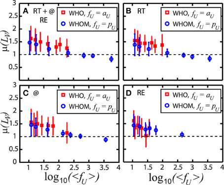
Figure 4. Mean μ of the local variation L_V of the user communication spike trains vs. the logarithmic average frequency log₁₀〈f_U〉. The results of who are represented by red squares and blue circles describe that of whom. Types of the interaction are investigated in detail: (A) All communications of retweet, RT, mention, @, and reply, RE. (B) Only RT. (C) Only @. (D) Only RE. Independent of the types of the interaction, the frequency of communication, e.g., the activity of users a_U and the popularity of users p_U, designs overall communication patterns. While low f_U gives bursty patterns with L_V > 1, moderate f_U indicates irregular uncorrelated (Poisson random) signals, e.g., L_V ≈ 1. For all high f_U, L_V < 1 presenting the regularity of the communications. The error bars show the corresponding standard variations.

We now perform a more thorough comparison in Figure 5, on the disparity of L_V in different frequency ranges. To this end, we calculate the standard z-values in two ways. First, to compare L_V of the full spike trains with L_V of only RT and also with L_V of only @ spike trains, $L_V^{RT}$ and $L_V^{@}$, respectively, we introduce

$\begin{array}{ll}z(f_U)=\frac{\mu (L_V^k)-{\mu }_0(L_V)}{\sigma (L_V^k)∕\sqrt{f_U^k}}& (3)\end{array}$

Here, k in superscripts labels the interaction, e.g., either RT or @. Precisely, $L_V^k$ is determined based on a filtered spike train composed of the user timestamps of either RT or @, as already used in (Figures 4B,C). In addition, μ^k is the mean of $L_V^k$, also presented in Figures 4B,C, and μ₀ is the mean L_V of the full spike train, given in Figure 4A.

FIGURE 5

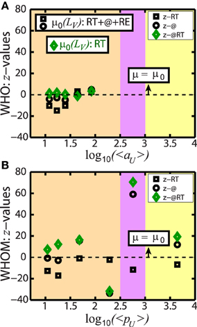
Figure 5. Detail comparison between the temporal patterns of different interactions in each frequency range. While x−axis is the logarithmic average of frequency, e.g., (A) log₁₀〈a_U〉 for who and (B) log₁₀〈p_U〉 for whom, y−axis provides the calculation of three z-values (i) z−RT in black squares, the comparison of L_V of the full spike train with L_V of RT, (ii) z−@ in black circles, the same with L_V of @, and (iii) z−@RT in green diamonds, the comparison between L_V of @ and RT. All z-values are consistent with each other such that except moderate frequency range in (B), e.g., z−@ and z−@RT, we observe small z concluding that the temporal patterns in the similar frequency ranges are in a good agreement. The three distinct regions are colored due to the discovered patterns in calculating L_V in Figure 4. Orange shaded area describes the ranges of the bursty patterns (a_U and low p_U), purple area is for the Poisson random dynamics (moderate p_U), and yellow area covers the regular patterns (high p_U).

In Figure 5, black squares show z-values of RT and black circles describe z-values of @. For who in Figure 5A where L_V only presents bursty patterns (orange shaded area) and low a_U, we have small z-values proving the agreement of the temporal patterns suggested by L_V in the same a_U. However, for whom in Figure 5B where we have rich values of p_U compared to the values of a_U, while z-values are small in bursty patterns (low p_U, orange area) as also in who and in regular patterns (high p_U, yellow area), larger z−@ value (the black circle) is calculated in uncorrelated Poisson dynamics (moderate p_U, purple area). The disagreement of L_V with large z−@ indicates that even though L_V ≈ 1 in this region the results of @ are quite sensitive in the same p_U, which is not observed in z−RT (the black square).

Furthermore, we repeat the analysis across communication channels by comparing temporal patterns of RT and @ as follows

$\begin{array}{ll}z(f_U)=\frac{\mu (L_V^{@})-{\mu }_0(L_V^{RT})}{\sigma (L_V^{@})∕\sqrt{f_U^{@}}}& (4)\end{array}$

The corresponding z-values, z−@RT are presented in green diamonds in Figure 5. Comparing to the previous z−RT and z−@, we now obtain even lower values for who (Figure 5A) showing a better agreement between RT and @ patterns. Moreover, we have a very similar trend for whom (Figure 5B) as before and so a large fluctuation is only observed in the purple area.

4. Correlation of L_V in User Communication Habits

In this final section, our interest turns into building new measures to quantify how the local variation L_V fluctuates inside different classes of the frequency, f_U. What extend temporal communication habits of two independent users in the same f_U ranges agree with each other is the first question we address. Second, we examine whether the temporal patterns of the interactions are consistent for the same users and how the metric varies with increasing f_U.

We consider $r_{ij}^{k{k}^{\prime }}(f_U)$, the Pearson correlation coefficient of L_V of two different users selected independently from the same f_U classes

$\begin{array}{ll}{r}_{ij}^{k{k}^{\prime }}(f_U)=\frac{{\displaystyle \sum _{i,j=1,i\ne j}^{N_U}}[L_{V_i}^k-\mu (L_{V_i}^k)][L_{V_j}^{k^{\prime }}-\mu (L_{V_j}^{k^{\prime }})]}{\sigma (L_{V_i}^k)\sigma (L_{V_j}^{k^{\prime }})}& (5)\end{array}$

where $\sigma (L_{V_i}^k)=\sqrt{{\displaystyle \sum _{i=1}^{N_U}}{\left[L_{V_i}^k-\mu (L_{V_i}^k)\right]}^2}$. Here, L_Vi and L_Vj are the local variations of user i and j, respectively, μ's are the corresponding mean values, and N_U is the total number of users. Moreover, k and k′ represent all permutations among the full, RT, and @ spike trains. Furthermore, $r_{ij}^{k{k}^{\prime }}(f_U)$ is evaluated for who and whom, separately. Therefore, i and j are different users, but from the same (who/whom) pool and in the same frequency classes of a_U and p_U, as grouped in Figure 3. Note that before performing Equation (5), the corresponding L_V's in the same f_U class are ordered from the highest to the smallest (or vice versa) not to deform $r_{ij}^{k{k}^{\prime }}(f_U)$ artificially due to the random selection.

Figure 6 presents the results of $r_{ij}^{k{k}^{\prime }}(f_U)$ for who in (a, b) and whom in (c, d). Similar to z-values performed in the previous Section, we suggest three correlation coefficients: Red (left) triangles describe $r_{ij}^{full,RT}$, blue (right) triangles are for $r_{ij}^{full,@}$, and black and green diamonds show the values of $r_{ij}^{RT,@}$. The average frequency of the users 〈f_U〉 in the same class is similar but not equal and that is why Figures 6B,D are plotted with respect to both the mean frequencies of RT and @, e.g., the average activity 〈a_U〉 and popularity 〈p_U〉 of RT and @. All correlations are above 0.85 proving the high dependency of the communication patterns of the users in the same 〈f_U〉, independently of the types of the interaction.

FIGURE 6

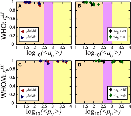
Figure 6. Linear correlations of L_V of user pairs. The standard Pearson correlation coefficient quantifies the dependency on the temporal communication habits of two different users independently chosen from the same frequency classes, as introduced in Figure 3. The coefficient covers 3 potential relations in the communication interactions, e.g., full and RT spike trains, red (left) triangles, full and @, blue (right) triangles, and finally RT and @, black and green diamonds. These 3 coefficients are calculated for who (A,B) and whom (C,D), separately. Six coefficients in total prove that the temporal patterns present high consistency in each average frequency classes, the activity 〈a_U〉 and the popularity 〈p_U〉. In (B,D), the corresponding coefficients are described with the sensitivity of the frequency classes since the average frequency in the class of RT is so similar, but not exactly equal to that of @. The colored areas are as defined in Figure 5 and characterize the three main regions of the temporal patterns of the individual user spike trains, e.g., bursts (orange), irregular random (purple), and regular patterns (yellow).

We now consider Equation (5) with imposing the same user and repeat the procedure above for the correlation coefficient

$\begin{array}{ll}{r}_i^{k{k}^{\prime }}(f_U)=\frac{{\displaystyle \sum _i^{N_U}}[L_{V_i}^k-\mu (L_{V_i}^k)][L_{V_i}^{k^{\prime }}-\mu (L_{V_i}^{k^{\prime }})]}{\sigma (L_{V_i}^k)\sigma (L_{V_i}^{k^{\prime }})}& (6)\end{array}$

Figure 7 summarizes the results of Equation (6). While Figures 7A,C are in parallel with that of Figure 6 with slightly lower correlations for @ (blue right triangles), distinct behavior is observed in Figures 7B,D. Low correlations in Figure 7B indicate that the same who users present different temporal behavior in RT and @. On the other hand, Figure 7D shows an interesting temporal habit of whom users. Having no remarkable dependency captured in low popular users, we show that the correlation increases with 〈p_U〉 describing that the popular users are addressed in RT and @ in a temporarily similar procedure.

FIGURE 7

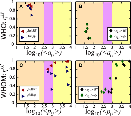
Figure 7. Linear correlations of L_V of the same users. The procedure and representation of the coefficients follow the same strategy as introduced in Figure 6. However, we now impose the same users in the same frequency classes. Even though (A,C) present the agreement in the temporal patterns of full and RT spike trains of the same users, with high correlation coefficients in almost all frequency ranges, (B) indicates lower consistency between RT and @ spike trains during entire activity 〈a_U〉 and (D) provides a significant result. While less temporal coherence is observed between RT and @ spike trains in low popularity 〈p_U〉, the correlation drastically increases with 〈p_U〉.

4.1. Nomenclature

• OSM: Online Social Media,

• @: Mention a user name in a tweet message,

• RE: Reply to a tweet or retweet message,

• RT: Retweet, share a message of other users in her/his own tweet blog,

• WHO: Twitter users starting an interaction via @ or RE or RT with any other users,

• WHOM: Twitter users addressed by who such that their message is retweeted or user name is mentioned in a message by who or they get a reply from who.

Any relation between who and whom such as the following-follower is not imposed.

5. Discussion

In this paper, our interest is to quantify online user communication in Twitter. To reduce the complexity in the communication, the data studied here consider only a unique subject which users talk about, that is the discovery of the Higgs boson on July 4, 2012 within a restricted time window, e.g., 6 days [38]. The main aim is to extract salient temporal patterns of communication in various types of interaction observed in Twitter such as retweet (RT), mention (@), and reply (RE). Adopting the technique so-called local variation L_V originally introduced for neuron spike trains [39–42] and recently has applied to hashtag spike trains in Twitter [43, 44], we perform detailed analysis on user communication spike trains. Showing strong influences of the frequency of the hashtag spike trains on the resultant temporal patterns in the earlier work [43, 44], in parallel we here examine the differences in the patterns induced by the frequency of the user communication spike trains, f_U.

We investigate user communication spike trains in two categories, the first set of users are the active ones, who users, and the other set is composed of the passive users, whom users, in the communication, and each user can appear in both pools. For who, f_U simply gives what extend users contact to whom and so it is the activity of who, a_U. On the other hand, for whom, the generated spike trains present how often who refers the messages or the user names of whom and therefore, f_U is the popularity of whom, p_U. Providing comparative statistics on L_V of who and whom with increasing a_U and p_U, respectively, we observe quite distinct temporal behavior of online users. First, we observe an asymmetry between active and passive interactions, as only the former give rise to hubs, with few users attracting a large share of the attention. Moreover, who constantly presents bursts, L_V > 1 for all values of a_U, whereas whom demonstrates various dynamic behavior patterns, depending on the popularity: The least popular users with low p_U experience bursty time series, popular users with moderate and high p_U are contacted by temporarily uncorrelated who users and so show Poisson random spike trains L_V ≈ 1, and the most popular users with the maximum p_U are referred regularly in time, e.g., L_V < 1.

These scenarios are independent of both the position of users, e.g., who or whom, and the preferred interactions, e.g., whether RT or @, suggesting that the frequency of the communication dominates to design social dynamic behavior. This conclusion is also supported by high correlation coefficients of L_V on the user pairs in the same frequency classes. Furthermore, the linear correlation of L_V on the same users reveals interesting patterns. There, we observe that only popular users have similar dynamic behavior in both RT and @, which confirms that both metrics are complementary to characterize the influence of users.

The analysis could be improved by integrating the communication spike trains with the following-follower relation in Twitter, and focusing on the who and whom trains of connected users. An important concern is the limited time period of the data which the collection started 3 days before the announcement of the discovery and continued until 3 days after this date. Yet, it has been shown that the dynamics of the communication is drastically different before/after and during the announcement [38], and this variation could be investigated in our analysis. Our study shares the similar aims of the other research on online user behavior and the influence of the frequency in online platforms such as Flickr, Delicious and StumbleUpon, which user profiles have been included in the analysis [47]. This understanding could be also applied to our analogy with considering further details in the data.

5.1. Data Sharing

The full data studied in this paper has open access [38, 45].

Author Contributions

Conceived and designed the experiments: CS. Performed the experiments: CS. Analyzed the data: CS. Contributed reagents/materials/analysis tools: RL, CS. Wrote the paper: CS, RL.

Funding

The EU 7th Framework OptimizR Project: 48909A2 CE OPTIMIZR (Grant holder: RL, Funding receiver: CS—http://optimizr.eu/) and FNRS MIS F4527.12 48888F3 (Grant holder: RL, Funding receiver: CS—http://www.fnrs.be/).

Conflict of Interest Statement

The authors declare that the research was conducted in the absence of any commercial or financial relationships that could be construed as a potential conflict of interest.

Acknowledgments

CS acknowledges supports from the European Union 7th Framework OptimizR Project and FNRS (le Fonds de la Recherche Scientifique, Wallonie, Belgium). This paper presents research results of the Belgian Network DYSCO (Dynamical Systems, Control, and Optimization), funded by the Interuniversity Attraction Poles Programme, initiated by the Belgian State, Science Policy Office.

References

1. Abisheva A, Garimella VRK, Garcia D, Weber I. Who watches (and shares) what on youtube? and when?: using twitter to understand youtube viewership. In: Proceedings of the 7th ACM International Conference on Web Search and Data Mining, WSDM '14. New York, NY: ACM (2014). pp. 593–602.

2. Wu S, Hofman JM, Mason WA, Watts DJ. Who says what to whom on twitter. In: Proceedings of the 20th International Conference on World Wide Web, WWW '11. New York, NY: ACM (2011). pp. 705–14.

3. Xuan Q, Gharehyazie M, Devanbu PT, Filkov V. Measuring the effect of social communications on individual working rhythms: a case study of open source software. In: Social Informatics (SocialInformatics), 2012 International Conference on. Washington, DC (2012). pp. 78–5.

4. Choudhury MD, Gamon, Counts, Horvitz. Predicting depression via social media. In: Kiciman E, Ellison NB, Hogan B, Resnick P, Soboroff I, editors. Proceedings of the Seventh International AAAI Conference on Weblogs and Social Media. Ann Arbor, MI: Association for the Advancement of Artificial Intelligence (AAAI) (2013). pp. 128–37.

5. Lambiotte R, Kosinski M. Tracking the digital footprints of personality. Proc IEEE (2014) 102:1934–9. doi: 10.1109/JPROC.2014.2359054

CrossRef Full Text | Google Scholar

6. Mathiesen J, Angheluta L, Ahlgren PTH, Jensen MH. Excitable human dynamics driven by extrinsic events in massive communities. Proc Natl Acad Sci USA. (2013) 110:17259–62. doi: 10.1073/pnas.1304179110

CrossRef Full Text | Google Scholar

7. Bakshy E, Hofman JM, Mason WA, Watts DJ. Everyone's an influencer: quantifying influence on twitter. In: Proceedings of the Fourth ACM International Conference on Web Search and Data Mining, WSDM '11. New York, NY: ACM (2011). pp. 65–74.

8. Gonzalez-Bailon S, Borge-Holthoefer J, Moreno Y. Broadcasters and hidden influentials in online protest diffusion. Am Behav Sci. (2013) 57:943–65. doi: 10.1177/0002764213479371

CrossRef Full Text | Google Scholar

9. Bakshy E, Karrer B, Adamic LA. Social influence and the diffusion of user-created content. In: Proceedings of the 10th ACM Conference on Electronic Commerce, EC '09. New York, NY: ACM (2009). pp. 325–34.

10. Lin YR, Bagrow JP, Lazer D. More voices than ever? quantifying media bias in networks. In: Nicolov N, Shanahan JG, editors. Proceedings of the Fifth International AAAI Conference on Weblogs and Social Media. Barcelona: Association for the Advancement of Artificial Intelligence (AAAI) (2011). pp. 193–200.

11. Kwon KH, Stefanone MA, Barnett GA. Social network influence on online behavioral choices: exploring group formation on social network sites. Am Behav Sci. (2014) 58:1345–60. doi: 10.1177/0002764214527092

CrossRef Full Text | Google Scholar

12. Zhang J, Tang J, Li J, Liu Y, Xing C. Who influenced you? predicting retweet via social influence locality. ACM Trans Knowl Discov Data (2015) 9:25:1–26. doi: 10.1145/2700398

CrossRef Full Text | Google Scholar

13. Lerman K, Yan X, Wu XZ. The majority illusion in social networks. ArXiv e-prints (2015) 1506.03022:1–10.

Google Scholar

14. Barabási AL. The origin of bursts and heavy tails in human dynamics. Nature (2005) 435:207–11. doi: 10.1038/nature03459

PubMed Abstract | CrossRef Full Text | Google Scholar

15. Goh KI, Barabasi AL. Burstiness and memory in complex systems. Europhys Lett. (2008) 81:48002. doi: 10.1209/0295-5075/81/48002

CrossRef Full Text | Google Scholar

16. Miritello G, Lara R, Moro E. Time allocation in social networks: correlation between social structure and human communication dynamics. In: Holme P, Saramaki J, editors. Temporal Networks. Berlin; Heidelberg: Springer (2013). pp. 175–90.

17. Formentin M, Lovison A, Maritan A, Zanzotto G. Hidden scaling patterns and universality in written communication. Phys Rev E (2014) 90:012817. doi: 10.1103/PhysRevE.90.012817

CrossRef Full Text | Google Scholar

18. Wang P, Lei T, Yeung CH, Wang BH. Heterogenous human dynamics in intra- and inter-day time scales. Europhys Lett. (2011) 94:18005. doi: 10.1209/0295-5075/94/18005

CrossRef Full Text | Google Scholar

19. Zhou T, Zhao ZD, Yang Z, Zhou C. Relative clock verifies endogenous bursts of human dynamics. Europhys Lett. (2012) 97:18006. doi: 10.1209/0295-5075/97/18006

CrossRef Full Text | Google Scholar

20. Colman ER, Greetham DV. Memory and burstiness in dynamic networks. Phys Rev E (2015) 92:012817. doi: 10.1103/PhysRevE.92.012817

CrossRef Full Text | Google Scholar

21. Karsai M, Kaski K, Barabási AL, Kertesz J. Universal features of correlated bursty behaviour. Sci Rep. (2012) 2:397. doi: 10.1038/srep00397

PubMed Abstract | CrossRef Full Text | Google Scholar

22. Jo HH, Perotti JI, Kaski K, Kertesz J. Correlated bursts and the role of memory range. Phys Rev E (2015) 92:022814. doi: 10.1103/PhysRevE.92.022814

PubMed Abstract | CrossRef Full Text | Google Scholar

23. Jo HH, Karsai M, Kertesz J, Kaski K. Circadian pattern and burstiness in mobile phone communication. New J Phys. (2012) 14:013055. doi: 10.1088/1367-2630/14/1/013055

CrossRef Full Text | Google Scholar

24. Kim J, Lee D, Kahng B. Microscopic modelling circadian and bursty pattern of human activities. PLoS ONE (2013) 8:e58292. doi: 10.1371/journal.pone.0058292

PubMed Abstract | CrossRef Full Text | Google Scholar

25. Iribarren JL, Moro E. Impact of human activity patterns on the dynamics of information diffusion. Phys Rev Lett. (2009) 103:038702. doi: 10.1103/PhysRevLett.103.038702

PubMed Abstract | CrossRef Full Text | Google Scholar

26. Lambiotte R, Tabourier L, Delvenne JC. Burstiness and spreading on temporal networks. Eur Phys J B (2013) 86:320. doi: 10.1140/epjb/e2013-40456-9

CrossRef Full Text | Google Scholar

27. Wang C, Huberman BA. How random are online social interactions? Sci Rep. (2012) 2:633. doi: 10.1038/srep00633

PubMed Abstract | CrossRef Full Text | Google Scholar

28. Formentin M, Lovison A, Maritan A, Zanzotto G. Universal activity pattern in human interactive dynamics. ArXiv e-prints (2014) 1405.5726:1–5.

Google Scholar

29. Ferrara E, Interdonato R, Tagarelli A. Online popularity and topical interests through the lens of instagram. In: Proceedings of the 25th ACM Conference on Hypertext and Social Media, HT '14. New York, NY: ACM (2014). pp. 24–34.

30. Ratkiewicz J, Fortunato S, Flammini A, Menczer F, Vespignani A. Characterizing and modeling the dynamics of online popularity. Phys Rev Lett. (2010) 105:158701. doi: 10.1103/PhysRevLett.105.158701

PubMed Abstract | CrossRef Full Text | Google Scholar

31. Coscia M. Competition and success in the meme pool: a case study on quickmeme.com. In: International AAAI Conference on Weblogs and Social Media (2013). pp. 100–9. Available online at: http://www.aaai.org/ocs/index.php/ICWSM/ICWSM13/paper/view/5990

32. Myers SA, Leskovec J. The bursty dynamics of the twitter information network. In: Proceedings of the 23rd International Conference on World Wide Web, WWW '14. New York, NY: ACM (2014). pp. 913–24.

33. ten Thij M, Ouboter T, Worm D, Litvak N, van den Berg H, Bhulai S. Modelling of trends in twitter using retweet graph dynamics. In: Bonato A, Graham FC, Pralat P, editors. Algorithms and Models for the Web Graph, Vol. 8882, of Lecture Notes in Computer Science. Springer International Publishing (2014). pp. 132–47. Available online at: http://dx.doi.org/10.1007/978-3-319-13123-8_11

34. Zhao Q, Erdogdu MA, He HY, Rajaraman A, Leskovec J. SEISMIC: a self-exciting point process model for predicting tweet popularity. In: Fayyad U, Cao L, Zhang C, editors. KDD15. Sydney: ACM (2015).

35. Boyd D, Golder S, Lotan G. Tweet, tweet, retweet: conversational aspects of retweeting on twitter. In: System Sciences (HICSS), 2010 43rd Hawaii International Conference on. Honolulu, HI (2010). pp. 1–10.

36. Zaman TR, Herbrich R, Gael JV, Stern D. Predicting information spreading in twitter. In: Computational Social Science and the Wisdom of Crowds Workshop (Colocated with NIPS 2010) (2010). Available online at: http://research.microsoft.com/apps/pubs/default.aspx?id=141866

37. Greetham DV, Ward. Conversations on twitter: structure, pace, balance. In: Kanawati R, Pensa RG, Rouveirol C, editors. Proceedings of the 2nd International Workshop on Dynamic Networks and Knowledge Discovery. CEUR Workshop Proceedings. Nancy (2014). pp. 73–84.

38. Domenico MD, Lima A, Mougel P, Musolesi M. The anatomy of a scientific rumor. Sci Rep. (2013) 3:2980. doi: 10.1038/srep02980

PubMed Abstract | CrossRef Full Text | Google Scholar

39. Shinomoto S, Shima K, Tanji J. Differences in spiking patterns among cortical neurons. Neural Comput. (2003) 15:2823–42. doi: 10.1162/089976603322518759

PubMed Abstract | CrossRef Full Text | Google Scholar

40. Miura K, Okada M, Amari S. Estimating spiking irregularities under changing environments. Neural Comput. (2006) 18:2359–86. doi: 10.1162/neco.2006.18.10.2359

PubMed Abstract | CrossRef Full Text | Google Scholar

41. Omi T, Shinomoto S. Optimizing time histograms for non-poissonian spike trains. Neural Comput. (2011) 23:3125–44. doi: 10.1162/NECO_a_00213

PubMed Abstract | CrossRef Full Text | Google Scholar

42. Shinomoto S, Kim H, Shimokawa T, Matsuno N, Funahashi S, Shima K, et al. Relating neuronal firing patterns to functional differentiation of cerebral cortex. PLoS Comput Biol. (2009) 5:e1000433. doi: 10.1371/journal.pcbi.1000433

PubMed Abstract | CrossRef Full Text

43. Sanli C, Lambiotte R. Local variation of hashtag spike trains and popularity in twitter. PLoS ONE (2015) 10:e0131704. doi: 10.1371/journal.pone.0131704

PubMed Abstract | CrossRef Full Text | Google Scholar

44. Sanli C, Lambiotte R. Local variation of collective attention in hashtag spike trains. In: Modeling and Mining Temporal Interactions: Papers from the 2015 ICWSM Workshop (2015). pp. 8–12.

Google Scholar

45. Leskovec J, Krevl A. SNAP Datasets: Stanford Large Network Dataset Collection (2014). Available online at: http://snap.stanford.edu/data

46. Saramaki J, Leicht EA, Lopez E, Roberts SGB, Reed-Tsochas F, Dunbar RIM. Persistence of social signatures in human communication. Proc Natl Acad Sci USA. (2014) 111:942–7. doi: 10.1073/pnas.1308540110

PubMed Abstract | CrossRef Full Text | Google Scholar

47. Meo Pd, Ferrara E, Abel F, Aroyo L, Houben GJ. Analyzing user behavior cross social sharing environments. ACM Trans Intell Syst Technol. (2014) 5:14:1–31.

48. Huberman BA, Romero DM, Wu F. Social networks that matter: twitter under the microscope. First Monday (2009) 14:1–9. doi: 10.5210/fm.v14i1.2317

CrossRef Full Text

49. Gonçalves B, Perra N, Vespignani A. Modeling Users' activity on twitter networks: validation of dunbar's number. PLoS ONE (2011) 6:e22656. doi: 10.1371/journal.pone.0022656

PubMed Abstract | CrossRef Full Text | Google Scholar

50. Weng L, Flammini A, Vespignani A, Menczer F. Competition among memes in a world with limited attention. Sci Rep. (2012) 2:335. doi: 10.1038/srep00335

PubMed Abstract | CrossRef Full Text | Google Scholar

51. Gleeson JP, Ward JA, O'Sullivan KP, Lee WT. Competition-Induced criticality in a model of meme popularity. Phys Rev Lett. (2014) 112:048701. doi: 10.1103/PhysRevLett.112.048701

PubMed Abstract | CrossRef Full Text | Google Scholar

52. Cetin U, Bingol HO. Attention competition with advertisement. Phys Rev E (2014) 90:032801. doi: 10.1103/PhysRevE.90.032801

PubMed Abstract | CrossRef Full Text | Google Scholar

53. Borge-Holthoefer J, Banos RA, Gonzalez-Bailon S, Moreno Y. Cascading behaviour in complex socio-technical networks. J Complex Netw. (2013) 1–22. doi: 10.1093/comnet/cnt006

CrossRef Full Text | Google Scholar

54. Jo HH, Pan RK, Kaski K. Time-varying priority queuing models for human dynamics. Phys Rev E (2012) 85:066101. doi: 10.1103/PhysRevE.85.066101

PubMed Abstract | CrossRef Full Text | Google Scholar