Hecke Groups, Dessins d'Enfants, and the Archimedean Solids

1. Introduction

Grothendieck's dessins d'enfants—bipartite graphs drawn on Riemann surfaces—arise with ever-increasing frequency in twenty-first century mathematical physics, appearing in e.g., the study of ${N}$ = 2 supersymmetric gauge theories [1–3], elliptically fibred Calabi-Yaus [4–6], toric conformal field theories [7, 8], topological strings [9, 10], and elsewhere. Given this growing ubiquity, it is valuable to study both the basic theory of dessins, and the applications of this theory to particularly significant cases. This paper aims to achieve both such goals, by first reviewing the mathematical results which connect dessins d'enfants to the theory of Hecke groups, before applying this work to the dessins for the so-called Archimedean solids. The hope is to provide a compendium of computational results to aid future research featuring these objects.

With the above in mind, let us begin our story by recalling that the Platonic solids are the convex polyhedra with equivalent faces composed of congruent convex regular polygons; these objects have been known and studied for millennia. These solids also appear in mathematical physics: for example, the symmetries of the Platonic solids are related to D-brane orbifold theories [11]. Now, more broadly, another well-known class of convex polyhedra are the Archimedean solids: the semi-regular convex polyhedra composed of two or more types of regular polygons meeting in identical vertices, with no requirement that faces be equivalent. There are three categories of such Archimedean solids: (I) the Platonic solids; (II) two infinite series solutions – the prisms and anti-prisms; and (III) 14 further exceptional cases.

In Magot and Zvonkin [12], a novel approach to the Archimedean solids was taken by interpreting the graphs of these solids as clean dessins d'enfants. By clean, we mean that all the nodes of one of the two possible colors of the bipartite graph have valency two [13, 14]. Now, the planar graph of any polytope can be interpreted as a clean dessin by inserting a black node into every edge of the graph, and coloring every vertex white. In this way, one can construct dessins for all the Archimedean solids. In each case, the underlying Riemann surface is the sphere ℂℙ¹, and the dessins are drawn in a planar projection.

In a parallel vein, trivalent clean dessins can be associated to conjugacy classes of subgroups of the modular group Γ = PSL(2, ℤ). (Recall that the modular group Γ ≡ Γ(1) is the group of linear fractional transformations $z\to \frac{az+b}{cz+d}$, with a, b, c, d ∈ ℤ and ad − bc = 1. The presentation of Γ is 〈x, y|x² = y³ = I〉.) To do so, we replace all n-valent vertices of the dessin with oriented n-gons. This constructs a Schreier coset graph, which displays the permutation action of generators x and y on each coset Gx_i of PSL(2, ℤ) = ⋃_iGx_i, i = 1, …, μ, where μ is the index of some subgroup G in PSL(2, ℤ) [15]. Generalizing, any clean dessin (not necessarily trivalent) can be associated with a conjugacy class of subgroups of a certain so-called Hecke group H_n, defined as having presentation 〈x, y|x² = yⁿ = I〉.

Once a Hecke subgroup G has been associated to the dessin in question, further results follow. For example, one can quotient the upper half plane by G to construct the surface ${H}$∕G. From this, one can construct a Belyi map (in a manner detailed in the main body of this paper), i.e., a holomorphic map to ℙ¹ ramified at only {0, 1, ∞}. To each Belyi map there corresponds a unique dessin; precisely the dessin with which we began! Hence, this chain of connections compactifies to a circle.

Returning now to the Archimedean solids, we see that, interpreting these as dessins, we should be able to explore the above circle of connections via explicit computations. Indeed, the Belyi maps associated to these dessins have already been computed in Magot and Zvonkin [12]; therefore, our task is to complete the circle by computing representatives of the conjugacy classes of Hecke subgroups associated to these objects. Not only will this provide an illustration of this aspect of the mathematical theory underlying dessins, but it will also provide a useful resource for further research in this area. Indeed, given that some dessins for the Archimedean solids have have already arisen in areas of mathematical physics (see for example [3, 4, 6]), it is not unreasonable to expect that such dessins will continue to manifest themselves in future research.

The structure of this paper is as follows. In Section 2 we present some technical details regarding Hecke groups and dessins d'enfants. We show that it is possible to interpret each clean dessin as the Schreier coset graph for a conjugacy class of subgroups of a certain Hecke group, and review the circle of connections mentioned above. In Section 3, we find the permutation representations for the conjugacy classes of subgroups of Hecke groups corresponding to every Archimedean solid, and provide an algorithm to compute explicit generating sets of matrices for representatives of these conjugacy classes in each case. In Section 4, we close with some conclusions, returning to the specific applications of this work in various subfields of mathematical physics.

2. Dessins d'Enfants and Hecke Groups

In this section, we review some essential details regarding both Hecke groups and clean dessins d'enfants. We begin by considering the modular group Γ ≅ H₃, as although this is isomorphic to only one particular Hecke group, it is by far the most well-studied, and we shall draw upon the presented results at several points in the ensuing discussion. Subsequently, we discuss Hecke groups more generally, before moving on to consider clean dessins and their associated Belyi maps. Note that the connection between trivalent dessins and the modular group is discussed in Jones and Singerman [16, 17], while the relation between Hecke groups and maps is discussed in e.g., [18]. With these results in hand, we describe how every clean dessin is isomorphic to the Schreier coset graph for a conjugacy class of subgroups of a Hecke group, and how the circle of connections closes via a correspondence between such subgroups and the Belyi maps for the original dessins.

2.1. The Modular Group

To begin, let us recall some essential details regarding the modular group Γ. This is the group of linear fractional transformations $\mathbb{Z}\ni z\to \frac{az+b}{cz+d}$, with a, b, c, d ∈ ℤ and ad − bc = 1. It is generated by the transformations T and S defined by:

$\begin{array}{cc}T(z)=z+1,S(z)=-1/z.& \left(1\right)\end{array}$

The presentation of Γ is 〈S, T|S² = (ST)³ = I〉, and we will later discuss the presentations of certain modular subgroups. The 2 × 2 matrices for S and T are as follows:

$\begin{array}{cc}T=\left(\begin{array}{cc}1& 1\\ 0& 1\end{array}\right),S=\left(\begin{array}{cc}0& -1\\ 1& 0\end{array}\right).& \left(2\right)\end{array}$

Letting x = S and y = ST denote the elements of order 2 and 3, respectively, we see that Γ is the free product of the cyclic groups $C_2=\langle x|x^2=I\rangle$ and $C_3=\langle y|y^3=I\rangle$. It follows that 2 × 2 matrices for x and y are:

$\begin{array}{cc}x=\left(\begin{array}{cc}0& -1\\ 1& 0\end{array}\right),y=\left(\begin{array}{cc}0& -1\\ 1& 1\end{array}\right).& \left(3\right)\end{array}$

With these details in hand, we can consider some important subgroups of Γ.

2.1.1. Congruence Modular Subgroups

The most significant subgroups of Γ are the congruence subgroups, defined by having the entries in the generating matrices S and T obeying some modular arithmetic. Some conjugacy classes of congruence subgroups of particular note are the following:

• Principal congruence subgroups:

$\Gamma \left(m\right):=\left\{A\in \text{SL}(2;\mathbb{Z});A\equiv \pm I\text{mod}m\right\}/\left\{\pm I\right\};$

• Congruence subgroups of level m: subgroups of Γ containing Γ(m) but not any Γ(n) for n < m;

• Unipotent matrices:

${\Gamma }_1\left(m\right):=\left\{A\in \text{SL}(2;\mathbb{Z});A\equiv \pm \left(\begin{array}{cc}1& b\\ 0& 1\end{array}\right)\text{mod}m\right\}/\left\{\pm I\right\};$

• Upper triangular matrices:

${\Gamma }_0\left(m\right):=\left\{\left(\begin{array}{cc}a& b\\ c& d\end{array}\right)\in \Gamma ;c\equiv 0\text{mod}m\right\}/\left\{\pm I\right\}.$

• The congruence subgroups

$\Gamma \left(m;\frac{m}{d},ϵ,\chi \right):=\left\{\pm \left(\begin{array}{cc}1+\frac{m}{ϵ\chi }\alpha & d\beta \\ \frac{m}{\chi }\gamma & 1+\frac{m}{ϵ\chi }\delta \end{array}\right);\gamma \equiv \alpha \text{mod}\chi \right\}$

for certain choices of m, d, ϵ, χ (see [4, 6]).

We note here that:

$\begin{array}{cc}\Gamma \left(m\right)\subseteq {\Gamma }_1\left(m\right)\subseteq {\Gamma }_0\left(m\right)\subseteq \Gamma .& \left(4\right)\end{array}$

In Section 3 of this paper, we shall remark on the connections between some specific conjugacy classes of congruence modular subgroups and the Archimedean solids.

2.2. Hecke Groups

We can now extend our discussion of the modular group Γ ≅ H₃ to the more general Hecke groups H_n. The Hecke group H_n has presentation 〈x, y|x² = yⁿ = I〉, and is thus the free product of cyclic groups $C_2=\langle x|x^2=I\rangle$ and $C_n=\langle y|y^n=I\rangle$. Note that Γ ≅ H₃ where Γ is the modular group; and that H_n is the triangle group (2, n, ∞). H_n is generated by transformations T and S now defined by:

$\begin{array}{cc}T(z)=z+{\lambda }_n,S(z)=-1/z,& \left(5\right)\end{array}$

where λ_n is some real number to be determined. The 2 × 2 matrices for these S and T are:

$\begin{array}{cc}T=\left(\begin{array}{cc}1& {\lambda }_n\\ 0& 1\end{array}\right),S=\left(\begin{array}{cc}0& -1\\ 1& 0\end{array}\right).& \left(6\right)\end{array}$

Letting x = S and y = ST as in our discussion of Γ, we see that 2 × 2 matrices for x and y are:

$\begin{array}{cc}x=\left(\begin{array}{cc}0& -1\\ 1& 0\end{array}\right),y=\left(\begin{array}{cc}0& -1\\ 1& {\lambda }_n\end{array}\right).& \left(7\right)\end{array}$

For H_n, we clearly have (ST)ⁿ = I, thereby constraining λ_n for a given n [19]. Diagonalising y to compute yⁿ explicitly places a constraint which allows for a solution of λ_n; we find the following general expression, as well as some important values for small n:

In particular, the λ_n are algebraic numbers.

2.2.1. Congruence Subgroups of Hecke Groups

By way of extension of the above discussion of subgroups of the modular group Γ, it is useful to consider congruence subgroups of Hecke groups. The Hecke groups are discrete subgroups of PSL(2, ℝ); in fact, the matrix entries are in ℤ[λ_n], the extension of the ring of integers by the algebraic number λ_n. Note that:

$\begin{array}{cc}{H}_n\subset \text{PSL}\left(2,\mathbb{Z}\left[{\lambda }_n\right]\right).& \left(9\right)\end{array}$

However, unlike the special case of the modular group, this inclusion is strict. With this point in mind, we can define the congruence subgroups of Hecke groups in the following way [19]. Let I be an ideal of ℤ[λ_n]. We then define:

$\begin{array}{cc}\begin{array}{l}\text{PSL}\left(2,\mathbb{Z}\left[{\lambda }_n\right],I\right)=\{\left(\begin{array}{cc}a& b\\ c& d\end{array}\right)\in \text{PSL}\left(2,\mathbb{Z}\left[{\lambda }_n\right]\right);\\ a-1,b,c,d-1\in I\}.\end{array}& \left(10\right)\end{array}$

By analogy, we also define:

$\begin{array}{cc}{\text{PSL}}^1\left(2,\mathbb{Z}\left[{\lambda }_n\right],I\right)=\left\{\left(\begin{array}{cc}a& b\\ c& d\end{array}\right)\in \text{PSL}\left(2,\mathbb{Z}\left[{\lambda }_n\right]\right);a-1,c,d-1\in I\right\}& \left(11\right)\end{array}$

$\begin{array}{cc}{\text{PSL}}^0\left(2,\mathbb{Z}\left[{\lambda }_n\right],I\right)=\left\{\left(\begin{array}{cc}a& b\\ c& d\end{array}\right)\in \text{PSL}\left(2,\mathbb{Z}\left[{\lambda }_n\right]\right);c\in I\right\}.& \left(12\right)\end{array}$

Then we can define the congruence subgroups H_n(m), $H_n^1\left(m\right)$, and $H_n^0\left(m\right)$ of H_n as follows:

$\begin{array}{cc}{H}_n\left(I\right)=\text{PSL}\left(2,\mathbb{Z}\left[{\lambda }_n\right],I\right)\cap H_n;& \left(13\right)\end{array}$

$\begin{array}{cc}{H}_n^1\left(I\right)={\text{PSL}}^1\left(2,\mathbb{Z}\left[{\lambda }_n\right],I\right)\cap H_n;& \left(14\right)\end{array}$

$\begin{array}{cc}{H}_n^0\left(I\right)={\text{PSL}}^0\left(2,\mathbb{Z}\left[{\lambda }_n\right],I\right)\cap H_n.& \left(15\right)\end{array}$

We have:

$\begin{array}{cc}{H}_n\left(I\right)\subseteq H_n^1\left(I\right)\subseteq H_n^0\left(I\right)\subseteq H_n.& \left(16\right)\end{array}$

By analogy with our discussion of the modular group, we define congruence subgroups of level m of the Hecke group H_n as subgroups of H_n containing H_n(m) but not any H_n(p) for p < m [20]. With these details regarding Hecke groups and their subgroups in hand, we can now consider their connections to clean dessins d'enfants.

2.3. Dessins d'Enfants and Belyi Maps

A dessin d'enfant in the sense of Grothendieck is an ordered pair 〈X, ${D}$〉, where X is an oriented compact topological surface and ${D}$ ⊂ X is a finite graph satisfying the following conditions [13]:

1. ${D}$ is connected.

2. ${D}$ is bipartite, i.e., consists of only black and white nodes, such that vertices connected by an edge have different colors.

3. X \ ${D}$ is the union of finitely many topological discs, which we call the faces.

We can interpret any polytope as a dessin by inserting a black node into every edge, and coloring all vertices white. This process of inserting into each edge a bivalent node of a certain color is standard in the study of dessins d'enfants and gives rise to so-called clean dessins, i.e., those for which all the nodes of one of the two possible colors have valency two. An example of this procedure for the cube is shown in Figure 1.

FIGURE 1

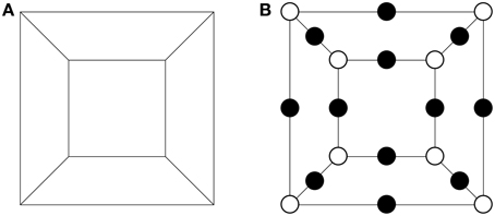
Figure 1. Interpreting the planar graph of the cube as a clean dessin. (A) The planar graph for the cube. (B) The corresponding clean dessin.

There is a one-to-one correspondence between dessins d'enfants and Belyi maps [13, 16, 17]. A Belyi map is a holomorphic map to ℙ¹ ramified at only {0, 1, ∞}, i.e., for which the only points $\tilde{x}$ where $\frac{d}{dx}\beta \left(x\right){|}_{\tilde{x}}=0$ are such that $\beta \left(\tilde{x}\right)\in \left\{0,1,\infty \right\}$. We can associate a Belyi map β(x) to a dessin via its ramification indices: the order of vanishing of the Taylor series for β(x) at $\tilde{x}$ is the ramification index $r_{\beta \left(\tilde{x}\right)\in \left\{0,1,\infty \right\}}\left(i\right)$ at that ith ramification point [4, 6]. To draw the dessin from the map, we mark one white node for the ith pre-image of 0, with r₀(i) edges emanating therefrom; similarly, we mark one black node for the jth pre-image of 1, with r₁(j) edges. We connect the nodes with the edges, joining only black with white, such that each face is a polygon with 2r_∞(k) sides [6]. The converse direction (from dessins to Belyi maps) is detailed in e.g., [13], and involves using the dessin to construct a so-called triangle decomposition of the surface X in which it is embedded, before constructing a unique Belyi function from that decomposition. For more information on dessins and Belyi maps, the reader is referred to Girondo and Gonzalez-Diez [13], Schneps [21], Lochak and Schneps [22, 23].

2.4. Belyi Maps from Hecke Subgroups

Let G be a torsion-free subgroup of the Hecke group H_n of finite index (i.e., a subgroup that contains no element of finite order other than the identity). Then, the compact surface X_G is obtained from the surface ${H}$∕G (where ${H}$ is the upper half plane) by adding finitely many points on the boundary real line of ${H}$, called cusps (in mathematical language: one for each G-orbit of boundary points at which the stabilizer is non-trivial). For example, choosing n = 3 and letting G be the full modular group Γ, there is a single cusp, equivalent to any rational number under G, namely, the point at infinity—this is the one-point compactification of the complex plane into the Riemann sphere. Then (returning to the general case), after carrying out this compactification, the holomorphic projection π : ${H}$∕G → ${H}$∕H_n ≅ ℂ extends to a Belyi map $\beta :X_G\to {\mathbb{P}}^1$, with each cusp of X_G mapped by β to the single cusp {∞} of H_n which compactifies the plane ${H}$∕H_n to ℂ∪∞ = ℙ¹ [24]. In turn, this Belyi map will have a unique associated dessin, as discussed in the previous section.

2.5. Schreier Coset Graphs

As mentioned, the Hecke group H_n has presentation 〈x, y|x² = yⁿ = I〉, and is thus the free product of cyclic groups $C_2=\langle x|x^2=I\rangle$ and $C_n=\langle y|y^n=I\rangle$. Given the free product structure of H_n, we see that its Cayley graph is an infinite free n-valent tree, but with each node replaced by an oriented n-gon. Now, for any finite index subgroup G of H_n, we can quotient the Cayley graph to arrive at a finite graph by associating nodes to right cosets and edges between cosets which are related by action of a group element. In other words, this graph encodes the permutation representation of H_n acting on the right cosets of G. This is called a Schreier coset graph, sometimes also referred to in the literature as a Schreier-Cayley coset graph, or simply a coset graph.

It is useful consider the permutations induced by the respective actions of x and y on the cosets of each Hecke subgroup; denote these by σ₀ and σ₁, respectively. We can find a third permutation σ_∞ by imposing the following condition, thereby constructing a permutation triple [16, 17]:

$\begin{array}{cc}{\sigma }_0·{\sigma }_1·{\sigma }_{\infty }=1.& \left(17\right)\end{array}$

The permutations σ₀, σ₁, and σ_∞ give the permutation representations of H_n on the right cosets of each subgroup in question. As elements of the symmetric group, σ₀ and σ₁ can easily be computed from the Schreier coset graphs by following the procedure elaborated in Sebbar [25], i.e., by noting that the doubly directed edges represent an element x of order 2, while the positively oriented triangles represent an element y of order n. Since the graphs are connected, the group generated by x and y is transitive on the vertices. Clearly, σ₀ and σ₁ tell us which vertex of the coset graph is sent to which, i.e., which coset of the Hecke subgroup in question is sent to which by the action of H_n on the right cosets of this subgroup.

Now, as detailed in Singerman and Wolfart [26], there is a direct connection between the Schreier coset graphs and the dessins d'enfants for each class of Hecke subgroups: the dessins d'enfants for a certain conjugacy class of subgroups of a Hecke group H_n can be constructed from the Schreier coset graphs by replacing each positively oriented n-gon with a white node, and inserting a black node into every edge. Conversely, the Schreier coset graphs can be constructed from the dessins by replacing each white node with a positively oriented n-gon, and removing the black node from every edge. Crucially, the dessin constructed in this way is the same dessin as that associated to the Belyi map for the surface X_G as discussed above, where G is the conjugacy class of Hecke subgroups under consideration [24, 26].

This last result means that our chain of connections between Hecke groups and dessins d'enfants has come full circle: for a given conjugacy class of subgroups G of a Hecke group H_n, there is an associated (compactified) surface X_G; in each case there exists a Belyi map $\beta :X_G\to {\mathbb{P}}^1$. Every such Belyi map has a unique associated dessin, which in turn can be translated into a Schreier coset graph for a certain conjugacy class of Hecke subgroups—precisely the G from which we began!

3. Hecke Subgroups and Archimedean Solids

Having reviewed the theory connecting dessins d'enfants with Hecke subgroups, we can now apply this theory to the particular case of the Archimedean solids. In this section, we first give a precise definition of these geometrical entities. We then identify the conjugacy class of Hecke subgroups corresponding to each Archimedean solid, by giving the permutation representations σ₀ and σ₁ for each such class. Finally, we discuss some interesting aspects of these results.

3.1. Platonic and Archimedean Solids

The Platonic solids are the regular, convex polyhedra; they are the tetrahedron, cube, octahedron, dodecahedron and icosahedron. In order to introduce the wider class of Archimedean solids, consider planar graphs without loops, and with vertices of degree k > 2. Following Magot and Zvonkin [12], let us call the list of numbers (f₁, f₂, …, f_k), where the f_i are the number of edges of the adjacent faces taken in the counter-clockwise direction around the vertex, the type of that vertex. Two such lists are equivalent if one can be obtained from the other by (a) making a cyclic shift and (b) inverting the order of the f_i. A solid is called Archimedean if the types of all its vertices are equivalent [12]¹.

We emphasize a subtlety here. One informal way of defining the Archimedean solids is as the semi-regular convex polyhedra composed of two or more types of regular polygons meeting in identical vertices, with no requirement that faces be equivalent. Identical vertices is usually taken to mean that for any two vertices, there must be an isometry of the entire solid that takes one vertex to the other. Sometimes, however, it is only required that the faces that meet at one vertex are related isometrically to the faces that meet at the other. On the former definition, the so-called pseudorhombicuboctahedron, also known as the elongated square gyrobicupola, is not considered an Archimedean solid; on the latter it is. The formal definition of the Archimedean solids above corresponds to the latter definition here; it is this latter definition which which we shall use.

The solids which satisfy the condition for being Archimedean are:

 I  The five Platonic solids;

 II  Two infinite series (the prisms and anti-prisms);

III  Fourteen exceptional solutions².

All these solids are listed in Table 1. For completeness, we also give the symmetry groups of each of these solids in the column labeled “Sym,” written in Schönflies notation. Here, we recognize the standard tetrahedral, octahedral and icosahedral groups:

$\begin{array}{cc}T\simeq A_4,O\simeq S_4,I\simeq A_5,& \left(18\right)\end{array}$

as well as the dihedral group D_n. The subscripts d and h denote extra symmetries about a horizontal (h) or diagonal (d) plane.

TABLE 1

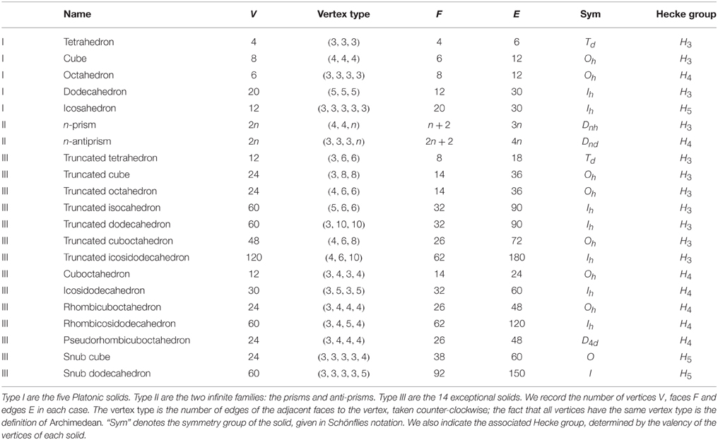
Table 1. The Archimedean solids.

3.2. Hecke Subgroups for the Archimedean Solids

As discussed, we can interpret all the Archimedean solids as clean dessins d'enfants by inserting a black node into every edge and coloring every vertex white. By the correspondences detailed in the previous section, we should then be able to associate a class of Hecke subgroups to every Archimedean solid. To achieve this, we begin by converting the dessins for these solids to Schreier coset graphs, reading off the associated permutations σ₀ and σ₁ for the conjugacy class of subgroups of the relevant Hecke group in each case; these results are tabulated in Appendix A. Next, we find a representative of the conjugacy class of subgroups of the relevant Hecke group in each case by inputting the permutations σ₀ and σ₁ into the GAP [31] algorithm presented in Appendix B. This yields a representative of the conjugacy classes of subgroups in each case.

To illustrate this procedure, consider the specific example of the octahedron. Inputting the permutations for the octahedron into the algorithm of Appendix B yields the following generators for a representative of the conjugacy class of subgroups of H₄ associated to this solid:

$\begin{array}{cc}\begin{array}{l}\{\left(\begin{array}{cc}-1& 0\\ 3\sqrt{2}& -1\end{array}\right),\left(\begin{array}{cc}1& -3\sqrt{2}\\ 0& 1\end{array}\right),\left(\begin{array}{cc}-7& -3\sqrt{2}\\ 6\sqrt{2}& 5\end{array}\right),\left(\begin{array}{cc}-7& -6\sqrt{2}\\ 3\sqrt{2}& 5\end{array}\right),\\ \left(\begin{array}{cc}5& -6\sqrt{2}\\ 3\sqrt{2}& -7\end{array}\right),\left(\begin{array}{cc}5& -3\sqrt{2}\\ 6\sqrt{2}& -7\end{array}\right),\left(\begin{array}{cc}11& -15\sqrt{2}\\ -15\sqrt{2}& 41\end{array}\right)\}.\end{array}& \left(19\right)\end{array}$

Note that comparison with our results concerning congruence subgroups of Hecke groups in Section 2.2 reveals that the octahedron corresponds to the principal congruence subgroup H₄(3). Repeating this procedure for all Archimedean solids, we find a number of results worthy of comment:

• While the octahedron corresponds to the conjugacy class of Hecke subgroups H₄(3), no other Archimedean solid is readily associated with congruence Hecke subgroups in an analogous manner.

• From Section 2.2, the matrices of H₄ are of the following two types:

$\begin{array}{cc}\left(\begin{array}{cc}a& b\sqrt{2}\\ c\sqrt{2}& d\end{array}\right),\left(\begin{array}{cc}a\sqrt{2}& b\\ c& d\sqrt{2}\end{array}\right)& \left(20\right)\end{array}$

The elements of the first type form a subgroup of index 2 in H₄; all the subgroups of H₄ corresponding to the Archimedean solids turn out to be subgroups of this subgroup.

• We have seen that, interpreted as dessins, the tetrahedron, cube and dodecahedron correspond to the conjugacy classes of subgroups Γ(3), Γ(4), and Γ(5), respectively [6]. In addition to these three arising as the dessins corresponding to certain congruence subgroups of the modular group, the dessins for the 33 conjugacy classes of genus zero, torsion-free congruence subgroups (discussed in detail in He et al. [6]) reveal that other Archimedean solids also correspond to certain conjugacy classes of congruence subgroups of the modular group. Specifically, the truncated tetrahedron is associated with the modular subgroup Γ₀(2) ∩ Γ(3), while the 8-prism is associated with the subgroup Γ(8;2, 1, 2). Given this, the question arises as to whether the other trivalent Archimedean solids can also be associated with congruence subgroups of the modular group. This can be checked in Sage [32] using the permutations σ₀ and σ₁ as input; doing so, we find that the answer to this question is in general negative. As a more specific result, we find that the truncated tetrahedron is the only trivalent, exceptional Archimedean solid which corresponds to a conjugacy class of congruence subgroups of the modular group.

4. Conclusions

In this paper, we have reviewed the connections between dessins d'enfants and Hecke subgroups. We have applied this theory to the case of the Archimedean solids, showing how, through interpretation as clean dessins, each of these geometric objects can be associated with a conjugacy class of subgroups of Hecke groups. In addition to opening up one more area of research into the Archimedean solids, this work is useful from the point of view of mathematical physics, as it can help to shed new light on cases where dessins naturally arise in physical contexts. To take two examples:

1. Certain ${N}$ = 2 supersymmetric gauge theories in four dimensions [33, 34] naturally give rise to trivalent dessins [3] (including Archimedean dessins); with the theory of this paper in mind, this suggests an otherwise overlooked connection between these gauge theories and modularity.

2. In He and McKay [4–6], it is shown that certain Calabi-Yaus give rise to clean, trivalent dessins, including many Archimedean dessins. Again, the theory of this paper therefore suggests a connection between the theory of Hecke groups and these Calabi-Yaus.

The general lessson is the following: given the growing ubiquity of dessins in mathematical physics, it is important to be clear and explicit on the connections of these objects to other areas of mathematics. Hence, it is important to illustrate the theory underlying these connections. It is particularly useful to lay out this theory explicitly in special cases such as that of the Archimedean solids, which we expect (on both inductive grounds and grounds of simplicity) to arise with greatest frequency in physical contexts.

Conflict of Interest Statement

The authors declare that the research was conducted in the absence of any commercial or financial relationships that could be construed as a potential conflict of interest.

The Reviewer Vishnu Jejjala, has previously published with an author of this manuscript, Dr He; the Editorial Office and Chief Editor confirm the review was carried out to the highest ethical standards.

Acknowledgments

YH thanks the Science and Technology Facilities Council, UK, for an Advanced Fellowship and for STFC grant ST/J00037X/1; the Chinese Ministry of Education, for a Chang-Jiang Chair Professorship at NanKai University; the city of Tian-Jin for a Qian-Ren Scholarship; the US NSF for grant CCF-1048082; as well as City University, London; the Department of Theoretical Physics, Oxford; and Merton College, Oxford, for their enduring support. JR is supported by an AHRC studentship at the University of Oxford, and is also indebted to Merton College for their support.

Footnotes

1. ^It is worth listing some classical sources on the Archimedean solids. Theses objects were first discussed by Archimedes, in a now lost work to which Pappus refers [27]. In the fifteenth century, the solids were rediscovered by Kepler [28]. Classical geometers who discuss the Archimedean solids include Sommerville [29] and Miller [27].

2. ^An interesting aside: It is known that the five Platonic solids correspond to three symmetry groups, which in turn are related to the exceptional Lie algebras E_{6, 7, 8}, and furthermore to Arnold's simple surface singularities with no deformations [30]. It is curious that the next order generalization of the simple singularities, with exactly one deformation modulus, has 14 exceptional cases. We conjecture, therefore, some connection to the exceptional Archimedean solids.

3. ^Of course, one should note that the octahedron and icosahedron could also be defined as subgroups of the modular group Γ, as their duals are trivalent.

References

1. Ashok S, Cachazo F, DellAquila E. Strebel differentials with integral lengths and Argyres-Douglas singularities. Preprint (2006). arXiv:hep-th/0610080.

Google Scholar

2. Ashok S, Cachazo F, DellAquila E. Children's drawings from Seiberg-Witten curves. Commun Number Theory Phys. (2007). 1:237–305. doi: 10.4310/CNTP.2007.v1.n2.a1

CrossRef Full Text | Google Scholar

3. He Y-H, Read J. Dessins d'enfants in ${N}$ = 2 generalised quiver theories. J High Energy Phys. (2015) 85:1–29. doi: 10.1007/JHEP08(2015)085

CrossRef Full Text | Google Scholar

4. He Y-H, McKay J. ${N}$ = 2 gauge theories: congruence subgroups, coset graphs and modular surfaces. J Math Phys. (2013) 54:012301. doi: 10.1063/1.4772976

CrossRef Full Text | Google Scholar

5. He Y-H, McKay J. Eta products, BPS states and K3 surfaces. J High Energy Phys. (2014) 2014:113. doi: 10.1007/JHEP01(2014)113

CrossRef Full Text | Google Scholar

6. He Y-H, McKay J, Read J. Modular subgroups, dessins d'enfants and elliptic K3 surfaces. LMS J Comput Math. (2013) 16:271–318. doi: 10.1112/S1461157013000119

CrossRef Full Text | Google Scholar

7. Hanany A, He YH, Jejjala V, Pasukonis J, Ramgoolam S, Rodriguez-Gomez D. The beta ansatz: a tale of two complex structures. J High Energy Phys. (2011) 1106:056. doi: 10.1007/JHEP06(2011)056

CrossRef Full Text | Google Scholar

8. Jejjala V, Ramgoolam S, Rodriguez-Gomez D. Toric CFTs, permutation triples and Belyi Pairs. J High Energy Phys. (2011) 1103:065. doi: 10.1007/JHEP03(2011)065

CrossRef Full Text | Google Scholar

9. Dumitrescu O, Mulase M, Safnuk B, Sorkin A. The spectral curve of the Eynard-Orantin recursion via the Laplace transform. In: Dzhamay A, Maruno K, Pierce VU, editors. Algebraic and Geometric Aspects of Integrable Systems and Random Matrices, Contemporary Mathematics, Vol. 593. Boston, MA: American Mathematical Society (2013). pp. 263–315.

10. Kazarian M, Zograf P. Virasoro constraints and topological recursion for Grothendieck's dessin counting. Lett Math Phys. (2015). 105:1057–1084. doi: 10.1007/s11005-015-0771-0

CrossRef Full Text | Google Scholar

11. Hanany A, He YH. Non-abelian finite gauge theories. High Energy Phys. (1999) 9902:013. doi: 10.1088/1126-6708/1999/02/013

PubMed Abstract | CrossRef Full Text | Google Scholar

12. Magot N, Zvonkin A. Belyi functions for Archimedean solids. Dis Math. (2000) 217:249–271. doi: 10.1016/S0012-365X(99)00266-6

CrossRef Full Text | Google Scholar

13. Girondo E, Gonzalez-Diez G. Introduction to Compact Riemann Surfaces and Dessins d'Enfants, London Mathematical Society Student Texts, Vol. 79. Cambridge, UK: Cambridge University Press (2012).

Google Scholar

14. Zvonkin A. Functional composition is a generalized symmetry. Symmetry (2011) 22:391–426.

PubMed Abstract

15. McKay J, Sebbar A. J-Invariants of arithmetic semistable elliptic surfaces and graphs. In: Proceedings on Moonshine and Related Topics. Montréal, QC (2001). pp. 119–30.

16. Jones GA, Singerman D. Theory of maps on orientable surfaces. Proc Lond Math Soc. (1978) 3–37:273–307. doi: 10.1112/plms/s3-37.2.273

CrossRef Full Text | Google Scholar

17. Jones GA, Singerman D. Belyi functions, hypermaps and Galois groups. Bull Lond Math Soc. (1996) 28:561–90. doi: 10.1112/blms/28.6.561

CrossRef Full Text | Google Scholar

18. Cangül I, Singerman D. Normal subgroups of Hecke groups and regular maps. Math Proc Camb Philos Soc. (1998) 123:59–74. doi: 10.1017/s0305004197002004

CrossRef Full Text

19. Ivrissimtzis I, Singerman D. Regular maps and principal congruence subgroups of Hecke groups. Eur J Comb. (2005) 26:437–456. doi: 10.1016/j.ejc.2004.01.010

CrossRef Full Text | Google Scholar

20. Ikikardes S, Sahin R, Cangul IN. Principal congruence subgroups of the Hecke groups and related results. Bull Braz Math Soc. (2009) 40:479–494. doi: 10.1007/s00574-009-0023-y

CrossRef Full Text | Google Scholar

21. Schneps L, (ed.). The Grothendieck Theory of Dessins D'enfants. London Mathematical Society Lecture Note Series, Vol. 200. Cambridge, UK: Cambridge University Press (1994).

Google Scholar

22. Lochak P, Schneps L, (eds.). Geometric Galois Actions 1. London Mathematical Society Lecture Note Series, Vol. 242. Cambridge, UK: Cambridge University Press (1997).

Google Scholar

23. Lochak P, Schneps L, (eds.). Geometric Galois Actions 2. London Mathematical Society Lecture Note Series, Vol. 243. Cambridge, UK: Cambridge University Press (1997).

Google Scholar

24. Harvey W. Teichmüller spaces, triangle groups and Grothendieck dessins. In: Papadopoulos A, editor. Handbook of Teichmüller Theory, Vol. 1. Zürich: European Mathematical Society (2007). pp. 249–292.

25. Sebbar A. Modular subgroups, forms, curves and surfaces. Can Math Bull. (2002) 45:294–308. doi: 10.4153/CMB-2002-033-1

CrossRef Full Text | Google Scholar

26. Singerman D, Wolfart J. Cayley graphs, Cori hypermaps, and dessins d'enfants. ARS Math Contemp. (2008) 1:144–53.

Google Scholar

27. Grünbaum B. An enduring error. Elem Math. (2009) 64:89–101. doi: 10.4171/EM/120

PubMed Abstract | CrossRef Full Text

28. Field J. Rediscovering the Archimedean polyhedra: Piero della Francesca, Luca Pacioli, Leonardo da Vinci, Albrecht Dürer, Daniele Barbaro, and Johannes Kepler. Arch Hist Exact Sci. (1997) 50. doi: 10.1007/BF00374595

CrossRef Full Text | Google Scholar

29. Sommerville DMY. Semi-regular networks of the plane in absolute geometry. Trans R Soc Edinb. (1906) 41:725–747. doi: 10.1017/S0080456800035560

CrossRef Full Text | Google Scholar

30. Brieskorn E, Pratoussevitch A, Rothenhäusler F. The combinatorial geometry of singularities and Arnold's series E, Z, Q. Mosc Math J. (2003) 3:273–333.

31. The GAP Group. GAP – Groups, Algorithms, and Programming, Version 4.5.6. (2012). Available online at: http://www.gap-system.org

32. Sage. Sage – Version 5.3. (2012). Available online at: http://www.sagemath.org

33. Gaiotto D. ${N}$ = 2 dualities. J High Energy Phys. (2012) 34:8. doi: 10.1007/JHEP08(2012)034

PubMed Abstract | CrossRef Full Text | Google Scholar

34. Tachikawa Y. ${N}$ = 2 supersymmetric dynamics for pedestrians. Lect. Notes Phys. (2014) 890. doi: 10.1007/978-3-319-08822-8

CrossRef Full Text | Google Scholar

Appendix

A. Permutations for the Archimedean Solids

In this appendix, we present the permutations σ₀ and σ₁ corresponding to the conjugacy classes of Hecke subgroups for each of the Archimedean solids. Although it is in principle easy to read these permutations off from the Schreier coset graphs in the manner detailed in Section 2.5, the procedure is extremely time-consuming, so it is worth presenting the results in full here. The method for computing explicit generators for a representative of each class of subgroups is detailed in the following appendix.

As a technical point, note that we have just presented the permutations σ₀ in each case. The permutations σ₁ can be written down by populating 2E∕n n-tuples with numerals in ascending order from 1 to 2E, where E is the number of edges of the solid, and H_n is the associated Hecke group as given in Table 1. So, for example, the permutations σ₁ for the octahedron are: (1, 2, 3, 4) (5, 6, 7, 8) (9, 10, 11, 12) (13, 14, 15, 16) (17, 18, 19, 20) (21, 22, 23, 24).

A.1. Platonic Solids

Interpreted as clean dessins d'enfants, the tetrahedron, cube, and dodecahedron correspond to the conjugacy classes of principal congruence subgroups Γ(3), Γ(4), and Γ(5), respectively [6]. In addition, from Table 1 we can see that the remaining two Platonic solids—the octahedron and the icosahedron—correspond to conjugacy classes of subgroups of H₄ and H₅, respectively³. The permutations σ₀ for these classes are:

Octahedron: (1, 5) (6, 11) (4, 12) (2, 13) (3, 23) (8, 14) (7, 18) (10, 19) (9, 22) (16, 24) (15, 17) (20, 21)

Icosahedron: (1, 6) (10, 11) (5, 15) (2, 21) (3, 16) (4, 43) (7, 22) (8, 27) (9, 33) (12, 34) (13, 37) (14, 42) (17, 25) (23, 26) (28, 32) (35, 36) (38, 41) (20, 44) (18, 46) (24, 47) (30, 48) (29, 52) (31, 53) (40, 54) (39, 57) (45, 58) (19, 59) (50, 60) (55, 56) (49, 51)

A.2. Prisms and Antiprisms

The prisms and antiprisms form infinite series of Archimedean solids. Since all prisms are trivalent, all correspond to a conjugacy class of subgroups of Γ; since all antiprisms are 4-valent, all correspond to a conjugacy class of subgroups of H₄. We can construct general expressions for the permutations σ₀ and σ₁ for the prisms and antiprisms. These expressions can be used to find the permutations σ₀ and σ₁ for any particular (anti)prism of interest.

Prisms:

Call the n-gon faced prism the n-prism. The n-prism has the following permutations σ₀ and σ₁:

$\begin{array}{cc}\begin{array}{l}{\sigma }_0:\left(3n-2,3\right)\left(3n-1,6n-2\right)\left(6n-1,3n+3\right)\\ ·{\displaystyle \prod _{i=0}^{n-2}\left(3i+1,3i+6\right)}\left(3i+2,3n+3i+1\right)\\ \left(3n+3i+2,3n+3i+6\right)\\ {\sigma }_1:{\displaystyle \prod _{i=0}^{n+2}\left(3i+1,3i+2,3i+3\right)}.\end{array}& \left(\text{A}1\right)\end{array}$

Antiprisms:

Call the n-gon faced anti-prism the n-antiprism. The n-antiprism has the following permutations σ₀ and σ₁:

$\begin{array}{cc}\begin{array}{l}{\sigma }_0:\left(4n-3,4\right)\left(4n-2,8n-2\right)\left(3,8n-1\right)\left(4n+1,8n\right)\\ ·{\displaystyle \prod _{i=0}^{n-2}\left(4i+1,4i+8\right)}\left(4i+2,4n+4i+2\right)\\ \left(4i+7,4n+4i+3\right)\left(4n+4i+4,4n+4i+5\right)\\ {\sigma }_1:{\displaystyle \prod _{i=0}^{n+2}\left(4i+1,4i+2,4i+3,4i+4\right)}.\end{array}& \left(\text{A}2\right)\end{array}$

A.3. Exceptional Archimedean Solids

In addition to the Platonic solids and the prisms and antiprisms, there remain 14 exceptional Archimedean solids, as given in Table 1. Here we give the permutations σ₀ for each corresponding class of Hecke subgroups.

Truncated tetrahedron: (1, 32) (3, 4) (2, 7) (5, 9) (6, 24) (8, 10) (11, 13) (12, 18) (15, 16) (17, 19) (14, 28) (29, 31) (33, 34) (30, 36) (26, 35) (20, 25) (23, 27) (21, 22)

Truncated cube: (3, 4) (2, 7) (5, 9) (60, 61) (63, 55) (57, 58) (20, 22) (21, 27) (24, 25) (11, 13) (12, 18) (15, 16) (39, 45) (43, 42) (38, 40) (30, 31) (29, 35) (32, 34) (66, 72) (65, 68) (67, 70) (48, 49) (47, 53) (50, 52) (1, 59) (62, 64) (69, 54) (51, 6) (41, 46) (8, 10) (56, 23) (36, 71) (33, 37) (17, 44) (14, 19) (26, 28)

Truncated octahedron: (1, 11) (2, 4) (5, 8) (9, 10) (12, 13) (3, 36) (6, 56) (7, 65) (35, 26) (32, 34) (29, 31) (27, 28) (25, 17) (16, 14) (15, 24) (21, 22) (18, 19) (23, 68) (70, 69) (66, 67) (62, 64) (63, 72) (59, 61) (57, 58) (51, 60) (50, 52) (54, 55) (49, 48) (45, 71) (20, 42) (30, 37) (39, 40) (38, 47) (44, 46) (41, 43) (33, 53)

Truncated icosahedron: (1, 14) (11, 13) (8, 10) (5, 7) (2, 4) (3, 16) (15, 28) (12, 26) (9, 22) (6, 20) (19, 35) (32, 34) (17, 31) (18, 58) (56, 60) (29, 55) (30, 53) (50, 52) (27, 49) (25, 47) (45, 46) (44, 23) (24, 41) (38, 40) (21, 37) (36, 73) (33, 64) (59, 61) (57, 110) (54, 107) (51, 98) (48, 95) (43, 86) (42, 83) (39, 77) (71, 75) (70, 68) (65, 67) (66, 62) (63, 116) (115, 113) (111, 112) (108, 109) (106, 104) (101, 103) (100, 99) (96, 97) (92, 94) (89, 91) (87, 88) (84, 85) (80, 82) (119, 79) (78, 118) (74, 76) (120, 122) (72, 164) (69, 158) (117, 155) (114, 149) (146, 105) (140, 102) (93, 137) (131, 90) (128, 81) (163, 161) (159, 160) (156, 157) (152, 154) (150, 151) (147, 148) (143, 145) (141, 142) (138, 139) (134, 136) (132, 133) (129, 130) (125, 127) (123, 124) (121, 165) (162, 166) (153, 179) (144, 176) (135, 173) (126, 170) (167, 169) (171, 172) (174, 175) (177, 178) (168, 180)

Truncated dodecahedron: (1, 29) (3, 32) (30, 31) (27, 44) (23, 25) (24, 43) (21, 41) (18, 40) (17, 19) (11, 13) (15, 39) (12, 38) (5, 7) (9, 35) (6, 34) (2, 4) (26, 28) (22, 20) (14, 16) (8, 10) (36, 62) (33, 46) (45, 107) (42, 92) (37, 77) (61, 59) (60, 66) (63, 64) (47, 49) (51, 120) (48, 119) (108, 109) (111, 105) (104, 106) (90, 96) (93, 94) (89, 91) (74, 76) (78, 79) (75, 81) (58, 56) (50, 52) (55, 53) (54, 122) (57, 123) (121, 136) (117, 118) (112, 110) (116, 113) (115, 135) (114, 134) (133, 149) (101, 103) (95, 97) (98, 100) (102, 131) (99, 130) (132, 146) (86, 88) (80, 82) (83, 85) (87, 128) (84, 127) (129, 142) (71, 73) (65, 67) (68, 70) (72, 126) (69, 125) (124, 139) (137, 154) (156, 153) (152, 138) (151, 180) (179, 150) (148, 176) (177, 178) (174, 175) (173, 147) (170, 145) (171, 172) (168, 169) (165, 166) (164, 144) (143, 167) (162, 163) (159, 160) (141, 158) (140, 161) (155, 157)

Truncated cuboctahedron: (1, 23) (24, 20) (21, 17) (18, 14) (15, 12) (10, 9) (7, 6) (4, 3) (2, 25) (22, 29) (19, 32) (16, 35) (13, 38) (11, 41) (8, 44) (5, 46) (26, 28) (30, 55) (56, 58) (31, 59) (33, 34) (36, 62) (63, 64) (65, 37) (39, 40) (42, 67) (68, 70) (43, 71) (45, 48) (47, 49) (50, 52) (27, 53) (54, 77) (51, 73) (76, 74) (78, 79) (75, 119) (57, 86) (60, 89) (88, 87) (85, 83) (90, 91) (61, 98) (66, 101) (100, 99) (95, 97) (102, 103) (72, 113) (69, 110) (111, 112) (114, 115) (107, 109) (80, 82) (84, 128) (126, 127) (81, 125) (129, 130) (132, 133) (96, 134) (92, 94) (93, 131) (135, 136) (137, 105) (104, 106) (108, 140) (138, 139) (141, 142) (117, 143) (123, 144) (120, 121) (116, 118) (122, 124)

Truncated icosidodecahedron: (1, 29) (26, 28) (23, 25) (20, 22) (17, 19) (15, 16) (11, 14) (8, 10) (5, 7) (2, 4) (3, 31) (30, 59) (27, 56) (24, 52) (21, 50) (18, 47) (13, 44) (12, 41) (9, 38) (6, 34) (33, 60) (58, 89) (88, 86) (85, 57) (53, 55) (83, 54) (80, 82) (79, 51) (48, 49) (46, 77) (75, 76) (45, 74) (42, 43) (40, 71) (68, 70) (39, 67) (35, 37) (36, 65) (64, 62) (61, 32) (90, 119) (87, 116) (84, 113) (81, 109) (78, 107) (73, 104) (72, 101) (69, 98) (66, 95) (63, 91) (93, 121) (123, 179) (178, 176) (175, 174) (173, 120) (118, 117) (115, 170) (169, 167) (166, 164) (163, 162) (161, 114) (112, 110) (111, 158) (155, 157) (152, 154) (149, 151) (108, 148) (105, 106) (103, 146) (143, 145) (140, 142) (138, 139) (102, 137) (99, 100) (97, 134) (131, 133) (128, 130) (125, 127) (96, 124) (92, 94) (122, 181) (180, 269) (177, 260) (257, 172) (171, 254) (168, 251) (165, 242) (160, 239) (159, 236) (156, 233) (153, 224) (150, 221) (147, 218) (144, 215) (141, 206) (136, 203) (135, 200) (132, 197) (129, 188) (126, 185) (184, 182) (183, 270) (268, 266) (265, 262) (264, 261) (259, 258) (256, 255) (252, 253) (248, 250) (247, 245) (244, 243) (241, 240) (237, 238) (234, 235) (230, 232) (227, 229) (226, 225) (222, 223) (219, 220) (216, 217) (214, 212) (209, 211) (207, 208) (204, 205) (202, 201) (199, 198) (196, 194) (191, 193) (189, 190) (186, 187) (267, 271) (263, 323) (249, 314) (246, 311) (231, 302) (228, 299) (290, 213) (210, 287) (195, 278) (192, 274) (276, 329) (328, 326) (325, 272) (273, 324) (322, 320) (319, 317) (316, 315) (313, 312) (308, 310) (307, 305) (304, 303) (300, 301) (296, 298) (293, 295) (291, 292) (288, 289) (284, 286) (281, 283) (279, 280) (275, 277) (330, 332) (327, 359) (321, 356) (353, 318) (350, 309) (347, 306) (344, 297) (294, 341) (285, 338) (282, 335) (333, 334) (331, 360) (358, 357) (355, 354) (351, 352) (348, 349) (345, 346) (342, 343) (339, 340) (337, 336)

Cuboctahedron: (1, 10) (11, 14) (15, 8) (4, 5) (2, 21) (3, 17) (20, 6) (7, 31) (30, 16) (27, 13) (22, 9) (12, 26) (25, 39) (28, 42) (43, 29) (32, 46) (47, 19) (18, 33) (24, 34) (23, 38) (35, 37) (40, 41) (44, 45) (36, 48)

Icosidodecahedron: (1, 9) (10, 17) (18, 26) (27, 34) (35, 4) (3, 37) (2, 5) (6, 12) (11, 13) (14, 20) (19, 21) (22, 25) (28, 29) (30, 33) (36, 40) (38, 41) (44, 79) (39, 78) (8, 45) (7, 49) (46, 52) (16, 54) (55, 57) (15, 58) (24, 63) (64, 65) (23, 66) (32, 70) (31, 74) (71, 73) (75, 77) (80, 110) (76, 109) (42, 48) (47, 82) (81, 43) (50, 53) (56, 86) (51, 85) (60, 93) (59, 62) (61, 94) (67, 69) (72, 102) (101, 68) (89, 96) (95, 100) (90, 99) (98, 107) (103, 108) (97, 104) (105, 112) (111, 116) (106, 115) (84, 113) (83, 117) (114, 120) (88, 118) (87, 92) (91, 119)

Rhombicuboctahedron: (1, 5) (6, 9) (10, 13) (4, 14) (2, 17) (3, 30) (20, 31) (8, 33) (7, 38) (34, 37) (12, 54) (11, 59) (55, 58) (15, 70) (67, 69) (16, 66) (18, 36) (35, 48) (21, 47) (19, 24) (40, 41) (39, 53) (50, 56) (42, 49) (57, 64) (61, 79) (68, 80) (65, 60) (72, 76) (28, 73) (25, 32) (29, 71) (22, 82) (27, 81) (23, 26) (44, 45) (46, 86) (43, 87) (51, 63) (62, 91) (52, 90) (75, 77) (74, 95) (78, 94) (84, 96) (83, 85) (88, 89) (92, 93)

Rhombicosidodecahedron: (1, 19) (4, 5) (8, 12) (11, 16) (15, 20) (2, 21) (3, 28) (6, 29) (7, 36) (9, 40) (10, 44) (13, 47) (14, 52) (17, 56) (18, 237) (240, 22) (24, 25) (27, 30) (32, 33) (35, 37) (39, 41) (43, 48) (46, 49) (51, 53) (55, 238) (54, 116) (57, 239) (23, 68) (26, 72) (31, 80) (34, 84) (38, 92) (42, 96) (45, 104) (50, 108) (115, 58) (60, 61) (64, 65) (67, 69) (71, 73) (76, 77) (79, 81) (83, 85) (88, 89) (91, 93) (95, 97) (100, 101) (103, 105) (107, 109) (112, 113) (114, 117) (175, 118) (62, 124) (63, 128) (66, 132) (70, 131) (74, 136) (75, 140) (78, 144) (82, 143) (86, 148) (87, 152) (90, 156) (94, 155) (98, 160) (99, 164) (102, 168) (106, 167) (110, 172) (111, 176) (119, 121) (123, 125) (127, 129) (130, 133) (135, 137) (139, 141) (142, 145) (147, 149) (151, 153) (154, 157) (159, 161) (163, 165) (166, 169) (171, 173) (59, 120) (122, 184) (126, 188) (134, 192) (138, 196) (146, 200) (150, 204) (158, 208) (162, 212) (170, 213) (174, 177) (183, 185) (187, 189) (191, 193) (195, 197) (199, 201) (203, 205) (207, 209) (211, 214) (178, 216) (180, 181) (182, 224) (186, 223) (190, 228) (194, 227) (198, 232) (202, 231) (206, 236) (210, 235) (215, 218) (179, 217) (222, 225) (226, 229) (230, 233) (234, 219) (220, 221)

Pseudorhombicuboctahedron: (1, 5) (6, 10) (11, 14) (4, 15) (2, 17) (3, 46) (20, 47) (8, 21) (7, 26) (22, 25) (9, 30) (12, 35) (31, 34) (13, 38) (16, 43) (39, 42) (18, 24) (23, 53) (50, 56) (19, 49) (28, 58) (59, 61) (32, 62) (27, 29) (33, 65) (66, 70) (40, 71) (36, 37) (44, 45) (48, 80) (76, 79) (41, 75) (52, 77) (51, 81) (84, 96) (78, 95) (55, 82) (83, 88) (60, 85) (54, 57) (86, 64) (63, 68) (67, 91) (87, 90) (89, 93) (73, 94) (72, 74) (69, 92)

Snub cube: (1, 18) (13, 17) (8, 12) (2, 7) (5, 22) (4, 60) (3, 53) (21, 19) (20, 26) (16, 35) (34, 14) (40, 15) (45, 11) (9, 44) (10, 49) (6, 54) (52, 56) (59, 23) (25, 27) (30, 31) (33, 36) (39, 41) (43, 50) (48, 55) (51, 73) (57, 72) (58, 67) (24, 61) (65, 28) (29, 97) (32, 93) (37, 92) (38, 87) (42, 84) (46, 83) (47, 78) (71, 68) (66, 62) (64, 98) (96, 94) (88, 91) (85, 86) (79, 82) (74, 77) (75, 108) (69, 107) (70, 103) (63, 102) (99, 101) (100, 119) (118, 95) (89, 117) (90, 114) (81, 113) (80, 112) (76, 109) (104, 106) (105, 120) (115, 116) (110, 111)

Snub dodecahedron: (1, 7) (8, 12) (13, 16) (17, 21) (5, 22) (2, 37) (3, 32) (4, 27) (6, 38) (10, 42) (9, 47) (11, 48) (15, 52) (14, 57) (20, 58) (19, 62) (18, 67) (25, 68) (24, 72) (26, 23) (28, 31) (33, 36) (39, 41) (43, 46) (49, 51) (53, 56) (59, 61) (63, 66) (69, 71) (30, 73) (29, 76) (35, 87) (34, 92) (40, 93) (45, 102) (44, 107) (50, 108) (55, 117) (54, 122) (60, 123) (65, 132) (64, 137) (70, 138) (75, 147) (74, 80) (77, 81) (82, 86) (88, 91) (94, 96) (97, 101) (103, 106) (109, 111) (112, 116) (118, 121) (124, 126) (127, 131) (133, 136) (139, 141) (142, 146) (79, 148) (149, 182) (78, 183) (85, 184) (84, 187) (83, 192) (90, 193) (89, 197) (95, 198) (100, 199) (99, 202) (98, 206) (105, 207) (104, 212) (110, 213) (115, 214) (114, 217) (113, 223) (120, 224) (119, 152) (125, 153) (130, 154) (129, 157) (128, 162) (135, 163) (134, 167) (140, 168) (145, 169) (144, 172) (143, 177) (150, 178) (200, 201) (203, 210) (208, 211) (215, 216) (218, 222) (225, 151) (155, 156) (158, 161) (164, 166) (170, 171) (173, 176) (179, 181) (185, 186) (188, 191) (194, 196) (195, 258) (205, 262) (204, 267) (209, 268) (220, 272) (219, 230) (221, 226) (160, 232) (159, 237) (165, 238) (175, 242) (174, 247) (180, 248) (190, 252) (189, 257) (259, 261) (263, 266) (269, 271) (273, 229) (227, 231) (233, 236) (239, 241) (243, 246) (249, 251) (253, 256) (260, 293) (265, 294) (264, 297) (270, 298) (275, 299) (274, 280) (228, 276) (235, 277) (234, 282) (240, 283) (284, 245) (287, 244) (288, 250) (289, 255) (292, 254) (295, 296) (300, 279) (278, 281) (285, 286) (290, 291)

B. Algorithm for Computing Generators for Hecke Subgroups

We can find the generators for a representative of all the conjugacy classes of subgroups of interest using GAP [6, 31]. First, we use the permutation data σ₀, σ₁ obtained from each of the Schreier coset graphs (in turn obtained from each of the dessins) to find the group homomorphism by images between the relevant Hecke group and a representative of the conjugacy class of subgroups of interest. We then use this to define the representative in question. Finally, we use the GAP command IsomorphismFpGroup(G), which returns an isomorphism from the given representative to a finitely presented group isomorphic to that representative. This function first chooses a set of generators of the representative and then computes a presentation in terms of these generators.

To give an example, consider the clean dessin for the octahedron. We can find a set of generators as 2 × 2 matrices for a representative of the associated class of subgroups by implementing the following code in GAP:

gap> f:=FreeGroup(“x”,“y”);
<free group on the generators [ x, y ]>
gap> H4:=f/[f.1^2,f.2^4];
<fp group on the generators [ x, y ]>
gap>hom:=GroupHomomorphismByImages(H4,Group(
(1,5)(6,11)(4,12)(2,13)(3,23)(8,14)(7,18)(10,19)(9,22)(16,24)(15,17)(20,21),
(1,2,3,4)(5,6,7,8)(9,10,11,12)(13,14,15,16)(17,18,19,20)(21,22,23,24)),
GeneratorsOfGroup(H4),
[(1,5)(6,11)(4,12)(2,13)(3,23)(8,14)(7,18)(10,19)(9,22)(16,24)(15,17)(20,21),
(1,2,3,4)(5,6,7,8)(9,10,11,12)(13,14,15,16)(17,18,19,20)(21,22,23,24))]);
[ x, y ] ->
[ (1,5)(2,13)(3,23)(4,12)(6,11)(7,18)(8,14)(9,22)(10,19)(15,17)(16,24)(20,21),
(1,2,3,4)(5,6,7,8)(9,10,11,12)(13,14,15,16)(17,18,19,20)(21,22,23,24) ]
gap> octahedron_group:=PreImage(hom,Stabilizer(Image(hom),1));
Group(<fp, no generators known>)
gap> iso:=IsomorphismFpGroup(octahedron_group);
[ <[ [ 1, 1 ] ]|y∗x∗y∗x^-1∗y∗x^-1>,
<[ [ 2, 1 ] ]|y^-1∗x∗y^-1∗x^-1∗y^-1∗x^-1>,
<[ [ 3, 1 ] ]|y^2∗x∗y∗x^-1∗y∗x^-1∗y^ -1>,
<[ [ 4, 1 ] ]|y^-1∗x∗y∗x∗y∗x^-1∗y^-2>,
<[ [ 5, 1 ] ]|x∗y^2∗x∗y∗x^-1∗y∗x^-1∗y^-1∗x^-1>,
<[ [ 6, 1 ] ]|x∗y^-1∗x∗y∗x∗y∗x^-1∗y^-2∗x^-1>,
<[ [ 7, 1 ] ]|y∗x∗y^-1∗x∗y∗x∗y^-1∗x^-1∗y∗x^-1∗y^-1∗x^-1> ]
-> [ F1, F2, F3, F4, F5, F6, F7 ]

We define the relevant Hecke group (here H₄) in the third line. Then, the only input in each case is the permutation data σ₀, σ₁. Once the output has been obtained, we see the generators (here seven: [F1, F2, F3, F4, F5, F6, F7]) in the final line, as functions of the x and y for the Hecke group in question. Now, returning to the explicit matrices for these x and y presented in Section 2.2, the only thing left to do is to multiply together the matrices and their inverses as indicated. This will produce the generators for each representative, as required.