Soft-Clamp Fiber Bundle Model and Interfacial Crack Propagation: Comparison Using a Non-linear Imposed Displacement

1. Introduction

Crack propagation in heterogeneous media is a rich problem which involves the interplay of various physical processes. The problem has been intensively investigated theoretically, numerically, and experimentally, but a unifying model capturing all the experimental features has not been entirely achieved [1, 2] despite its broad range of implications in engineering and Earth sciences problems [3, 4].

During most regular fracture experiments, the fracture surface can only be observed post mortem [5]. Since Mandelbrot's discovery [6] of fracture surfaces in metal that display fractal properties, there have been many attempts to understand the scaling relations of fracture [5]. In particular, the self-affine nature of fracture surfaces have come under much scrutiny. A self-affine surface h(x) has the following scaling relation [7]

$\begin{array}{cc}h(x)\propto {\lambda }^{\zeta }h(\lambda x),& (1)\end{array}$

where λ is an arbitrary scaling factor and ζ is the roughness exponent.

The slow propagation of a crack front where long range elastic interactions are dominant, is of crucial importance to fill the gap between experiments and models. In an attempt to study the in-situ properties of this process, Schmittbuhl and Måløy [8-10] developed an experiment where they forced the fracture to advance along a weak heterogeneous plane embedded in a transparent medium (Plexiglas). In such an experimental configuration, the propagation of the fracture front can be monitored in great detail using high resolution optical devices from which different properties characterizing the fracture dynamics can be inferred. For instance, the distribution of the local fracture velocities [11] or the multi-scale morphology of the fracture front [12] can notably be measured and are found to be robust parameters when tested against several experimental conditions.

Several theoretical and numerical studies have been devoted to quasi-static models [1, 13]. Such models give rise to an intermittent local activity characterized by a depinning transition and can be viewed as a critical phenomenon [2, 14, 15]. However, these models do not provide a complete modeling of the system as they fail to reproduce all the experimental observations. Notably the front morphology in these models does not display a cross-over length scale with two different roughness exponents above and below it. Such a cross-over was observed experimentally in 2010 by Santucci et al. [12]. They found that the in-plane fractures also had a scale-dependent roughness exponent. At small scales they obtained ζ⁻ = 0.60, while at large scales they showed that ζ⁺ = 0.35. Attempts to model the behavior of the in-plane fracture process had a long time resulted in only the large scale roughness exponent [16, 17], or the small scale roughness exponent in the context of a stress-weighted percolation [18]. Moreover, the scaling relations for fractures have now been established as being both scale and direction dependent [19-22].

Recently, Gjerden et al. [23, 24] presented for the first time roughness exponents compatible with both the large scale and small scale values found in the experiments. Their model was a development of the soft clamp fiber bundle model [25, 26] first introduced by Batrouni et al. [27]. Gjerden et al. implemented this model with a linear spatial gradient in the threshold distribution thereby creating a crack front whose dynamics and morphology could be compared to the experimental observations [24].

Even though the characteristics of the crack front that was created in the soft clamp fiber bundle model through the introduction of a linear gradient matched the experimental observations well, it cannot be ignored that the crack front was generated in a very different way in the experiment. It is therefore important to implement the same boundary conditions in the soft clamp model as was used in the experiments to test whether this change does lead to different results. This is the primary aim of this paper.

We also push further the comparison between theory and experiments, by focusing essentially on (i) the roughness exponent ζ that characterizes the geometry of the front at some given time (ii) the dynamic exponent κ that characterizes the time evolution of the crack front roughness and (iii) the statistics of the velocity fluctuations that show a scaling behavior with an exponent η that is still poorly understood. We note in particular that κ was not measured directly by Gjerden et al.[24], but rather inferred from assuming that the Family-Vicsek scaling assumption holds.

In the following, we first review in Section 2 the main aspects of the experimental setup. In Section 3, we give details on the numerical model based on the soft clamp fiber bundle approach but modified to include both long range elastic interactions owing to the elactically deformable clamped block and a non-linear imposed displacement around the process zone. In Section 4, we compare the experimental observations and numerical results. The predictions of the transient and steady-state scaling of the front morphology is discussed in the light of the experimental evidences. Finally the comparison of the local crack front velocity distribution is presented.

2. Experimental Setup

We compare our numerical results to experimental results obtained with the following setup. It consists of two transparent welded plexiglas (PMMA - poly methyl methacrylate) plates [e.g., 8, 11, 28, 29]. Disorder in the strength of the interface between the two plates is introduced by sandblasting using glass beads of variable diameters (180–300 μm), the opposite surfaces of the two plates that are to be welded together. Welding of the two plates is then achieved by imposing a normal load on the assembled plates while heating the system at 190°C. This thermal annealing produces a cohesive interface weaker than the bulk, along which the sample will break apart under normal opening loading. When the system is loaded from one side, a propagating crack—a fracture front—evolves that moves away from the loaded side. It is this crack we focus upon.

The dimensions are typically 20 cm long, 3 cm wide and 5 mm thick for the bottom plexiglas plate and 1 cm thick for the upper plate. The upper plate is attached to a stiff aluminum frame while a load is applied over the top side of the bottom plate in a direction normal to the plate interface. The vertical displacement imposed on the bottom plate induces stable mode I propagation of a planar fracture along the prescribed weak interface (mode II and III components related to the finite size of the sample and friction along the loading rod are neglected). A sketch of the experiment is given in Figure 1.

FIGURE 1

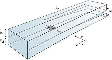
Figure 1. Sketch of the experimental setup. Two PMMA plates of thickness h₁ and h₂ are welded and a mode I fracture propagates at the interface between the two plates. Fracture propagation is caused by the opening, M, between the two plates. The distance between the loading point and the crack front is noted L_a. The crack front propagates along the y direction. The gray rectangle marks the area around the crack front (see Figure 2) we will reproduce in our simulations.

The fracture front creates an optical contrast between the broken and unbroken sections of the interface [28]. This fracture front is then tracked by an optical digital camera (a Nikon D700 with a resolution of 4256 × 2832 pixels at up to 5 images/s for slow monotoring or an Optronis Camrecord 600 with a resolution of 1000 × 1000 pixels at 1000 images/s for fast tracking) in order to extract its position through time [29-31]. The front propagates along the y axis where the origin is defined at the loading point and is positive in the direction of crack propagation (see Figures 1, 2). The x axis is perpendicular to y and defines the coordinate of a point along the front. The large scale bending of the plate at the sample size is well reproduced by the elastic beam theory [29]. At a smaller scale i.e., at the scale of the process zone, the elastic beam theory might however not be any more valid in describing the shape of the plate and typical crack solutions eventually provide more a realistic description as discussed below.

FIGURE 2

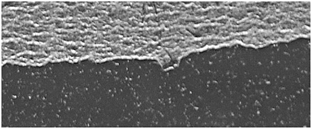
Figure 2. Picture of the crack front area obtained during an experiment. The crack is propagating from top to bottom, the gray part refers to already broken part and the dark area to the unbroken part. The optical contrast between this two parts defines the fracture front. The dimension of the picture in the x-direction is 4 mm.

3. Model

The soft clamp fiber bundle model was first introduced by Batrouni et al. [27] in 2002. We use this model in order to reproduce the phenomena occurring at the process zone scale around the fracture front by introducing the appropriate boundary conditions. We are indeed interested in describing the behavior of the fracture front on a short range from its edge. We thus consider our model as a square of dimension L_f × L_f around the fracture front. This area of the system is illustrated in Figure 1 by the dark square covering a part of the fracture front. This area is divided into N × N sub-squares, each of them containing a single fiber. A discretization size is then dl = L_f/N. The two facing Plexiglas plates are represented as infinite facing half-spaces, and act as clamps attached to the N² fibers. The half spaces are supposed to have an elastic behavior with a Youngs modulus E and a Poisson ratio of ν. An equivalent simpler configuration can be obtained by assuming that one of the half spaces is infinitely stiff. Thus, E will only describe the elastic response of the other half-space. The system is periodic along the x-axis.

The fibers are linearly elastic up to a strength threshold where they break irreversibly and can no longer support any load. On the contrary to Gjerden et al. [24], the thresholds are uniformly spatially distributed between $f_{min}^t$ and $f_{max}^t$, where we have set $f_{min}^t=0$ and $f_{max}^t=1$. The force, f_i, experienced by each individual fiber is given by the Hooke's law:

$\begin{array}{cc}{f}_i=-k(u_i-D_i),& (2)\end{array}$

where i is the index of the fiber, k is the spring constant, equal for all the fibers, D_i is the local position of the rigid plate (e.g., constant for all fibers if the plate is plane and horizontal), u_i is the local displacement of the facing soft elastic half-space created by the strain around the fiber by of this elastic half-space. When D_i = u_i, i.e., the imposed displacement is balancing the strain in the elastic half-space, the force in the fiber is nil. The spatially dependent deformation is calculated by Love's law [32]:

$\begin{array}{cc}{u}_i={\displaystyle \sum _{j\ne i}^{N^2}{G}_j}{f}_j& (3)\end{array}$

where j runs over all the fibers in the array (except the self-induced contribution). The Green function G_j is given by:

$\begin{array}{cc}{G}_j=\frac{1-{\nu }^2}{\pi Ed{l}^2}{\displaystyle {\int }_{-dl/2}^{+dl/2}{\displaystyle {\int }_{-dl/2}^{+dl/2}\frac{dx\prime dy\prime }{|{\overrightarrow{r}}_i(0,0)-{\overrightarrow{r}}_j(x\prime ,y\prime )|}}},& (4)\end{array}$

Integrals in Equation (4) run over each dl² square associated with the fiber j. The x′ and y′ coordinates have their origin in the middle of the discretization area. The vector ${\overrightarrow{r}}_i(x\prime ,y\prime )$ represents the position of the fiber i. E and ν are respectively the Young and Poison coefficients.

During loading in the experiments, the large scale mode I opening, induced by the imposed displacement of the bottom plate, is well reproduced by an elastic beam model [30]. On the contrary, at the process zone scale around the crack tip, the opening is strongly influenced by the fracture mechanics [3]. The opening of the crack δ(y) is then expected to have a square root shape behind the crack front [33]:

$\begin{array}{cc}\delta (y_c-y)=\frac{8(1-{\nu }^2)}{\sqrt{2\pi }}\left(\frac{K}{E}\right)\sqrt{y_c-y}& (5)\end{array}$

where y_c is the average position of the crack tip and K is the stress intensity factor.

Since our investigations focus on the small scales around the fracture front, we assume that elastic crack opening is dominant. Accordingly, we introduced a square root shape of the rigid plate (see Figure 3). The imposed displacement D(y) to the fiber bundle is then proposed to be proportional to the square root of the distance y_c − y to the fracture front [33].

FIGURE 3

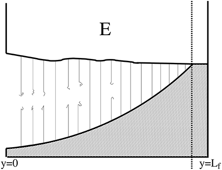
Figure 3. Sketch of the loading of the fiber-bundle model. Individual fibers are represented by dark vertical lines and can be broken or unbroken. The upper plate is the soft elastic block with a Young modulus E. The shape of the rigid bottom plate follows the displacement $D\propto \sqrt{L_f-y}$, as given by Equation (5).

We tested the approach using a non-linear shape of the rigid plate by considering a system with half of the fibers broken (see insert of Figure 4) and computing the resulting opening δ(y) = D(y) − u(y) in the domain of broken fibers, in the limit of infinite strength of the surviving fibers in the rest of the domain. We compared the configuration of a flat shape D(y) = D₀ and a square root shape $D(y)=D_0\sqrt{L_f-y}$ of the rigid plate (see Figure 4). The red line shows the opening field δ(y) between the rigid and the elastic clamps as a function of y for a system of size N = 256. The linear crack tip fracture front is at y_c = 129.

FIGURE 4

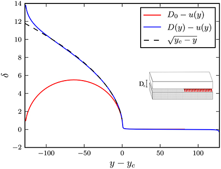
Figure 4. Insert: sketch of the half broken configuration considered in the figure in the case of a flat rigid plate (gray) facing a soft elastic block (white). Fibers in red are only set in the right half of the system. For this test, there are supposed to have an infinite strength, i.e., no possible failure). Main figure: Crack tip opening, δ(y), as a function of the distance to the first intact fiber, y_c. Two cases are considered for the imposed shape of the rigid plate: a flat shape in red and a crack-like shape in blue. A square-root crack fit is displayed as a black line.

When we fit the opening δ(y) with a square root shape similar to Equation (5), we see the difference between both configurations. In the case of a flat plate, the relation only holds in the immediate vicinity of the crack tip. As we increase the distance back to the front, δ(y) soon deviates from the theoretical crack tip opening. This deviation mostly results from the periodic property of the flat shape. With a square root shape illustrated by the blue line in Figure 4, the resulting crack tip opening is nicely fitted by Equation (5) and holds for a much larger portion of the system, over all the process zone of the front.

The force experienced by the fibers ahead of the crack tip for the different loading scheme is shown in Figure 5. We observe, for both the flat and square-root rigid plate shape that the force on the fibers, depends on the distance from the crack tip as an inverse square root profile consistently with elastic crack theory [3]. As we can see from the figure, the imposed square-root shape improves significantly the system compliance except at very large distance ahead of the crack front preventing failure of the fibers in this domain.

FIGURE 5

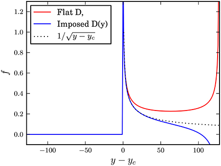
Figure 5. Profile of the force f(y) applied on the fibers ahead of the crack tip for two shapes of the rigid plate (flat in red or square root in blue) in a configuration similar to Figure 4.

We see from both Figures 4, 5 that the loading and the respond of the model become non-physical close to the boundaries of the system. In order to keep the process zone around the fracture tip away from the boundaries, we used the “conveyor belt” technique [34]. Since only the surviving fibers matter in the force field calculations and fibers fail irreversibly, we remove the first broken (i.e., left side in Figure 3) row from our calculations and add a fully intact one at the last (i.e., right side) row. n_c is the number of times a new intact row is introduced during the computation.

We prevented the last (1/2)Nlog(N) rows of fibers from breaking in order to prevent wrap-around of the failed fibers due to the periodic boundary conditions. For L = 256, this meant that four rows were unbreakable.

During the computation of the crack front advance, the system is updated iteratively and quasistatically by removing the fibers one by one following en event-driven algorithm [16]. At each step we compute a new prefactor D₀ that will correspond to a force field where only one of the fibers is experiencing a force equal to its strength threshold. This fiber is actually the closest one to failure and thus requires the least increase of D₀ to break. The fiber is then removed and the procedure is continued until there is no intact fiber left.

When the distances are measured in units of the discretization size dl, the relative influence of the elastic interactions with respect to the global loading has been found to be described by a single parameter named the reduced Young modulus [35]

$\begin{array}{cc}e=\frac{Edl}{N}.& (6)\end{array}$

where E is the Young modulus, N the number of fibers per system length L_f. Indeed, the contribution of the Green function in the force computation of each fiber can be turned on or off, depending on the value e. In the stiff regime, i.e., large e, the fracture process is dominated by a diffusive damage controlled by the strength heterogeneities in the system. When e decreases, the system goes through a cross-over regime where the influence of the elastic forces rises. When e is sufficiently low, the competition between the elastic redistribution and the strength heterogeneities are balanced and the system enters a so-called soft regime. This regime is dominated by localized damage. As we can see from Equation (6), decreasing E, while increasing N in a way that keeps e constant is not affecting the influence of the Green function. We will thus associate the soft systems with large length scales. Similarly, we will associate the stiff systems with short length scales.

4. Results

4.1. Front Morphology: Self-Affine Scaling and Cross-Over Length Scale

Previous experimental studies reported that an interfacial crack front in the present configuration is self-affine with a roughness exponent ζ≃ 0.6 [e.g., 8, 28]. More recent data extracted from numerous experiments and at various scales show that actually two distinct regimes emerge depending on the scale of investigation: at small scales the scaling regime is characterized by a roughness exponent ζ⁻ ≃ 0.60 while at large scale the exponent is lower and is found around ζ⁺ ≃ 0.35 [12]. We aim at a direct comparison of the scaling properties of the simulated crack front and the experimental observations. For this, we identify the fracture front as the interface between the cluster of broken fibers spacially connected (i.e., in the sense of a link between first neighbors) to one side of the system and the cluster of surviving fibers connected to the other side. When this interface is identified, it is approximated as a function of the x-coordinate for each time step t: h(x, t) by using a solid-on-solid (SOS) algorithm. The front line is indeed deduced by taking the first y-value hit when searching along the y-axis from above or below. An example of this front is given by the red line in Figure 6 for stiff systems, and in Figure 7 for soft systems.

FIGURE 6

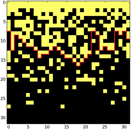
Figure 6. Example of process zone during a simulation for a stiff system (e = 62.5). The dark points refer to broken fibers while yellow points are intact fibers. The system size is N = 32.

FIGURE 7

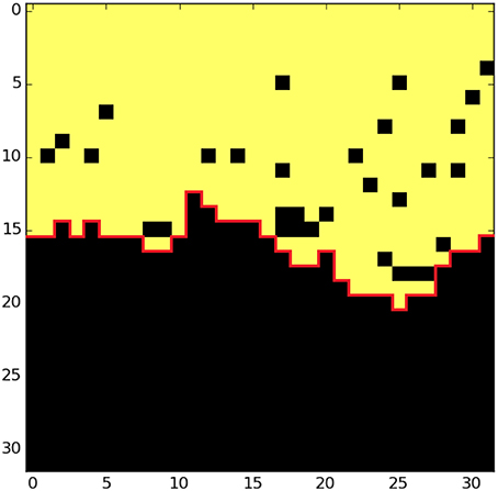
Figure 7. Same as Figure 6 for a soft system (e = 7.6·10⁻⁶).

We investigated the scaling properties of the crack front morphology in our simulations in a similar way to the experiments. In order to find the roughness exponent (cf Equation 1) of the fracture fronts produced by our model, we analyzed them using the average wavelet coefficient method which is shown to be very efficient for data over a limited range of scales [36]. The average wavelet coefficient W(a) is defined as:

$\begin{array}{cc}W(a)={\langle W(a,b)\rangle }_b& (7)\end{array}$

where a is the scale factor of the wavelet transform and b is the translation factor. It scales for a self-affine front as

$\begin{array}{cc}W(a)\propto a^{\zeta +1/2}.& (8)\end{array}$

In Figure 8, we see the average wavelet coefficient (using Daubechies wavelets of order 4) for the stiff regime for different system sizes. We find the roughness exponent of the small systems by making a fit over the three smallest coefficients. We exclude the very smallest, as the discretization size begins to influence the results. This gives us a roughness exponent of ζ₋ = 0.53 ± 0.02.

FIGURE 8

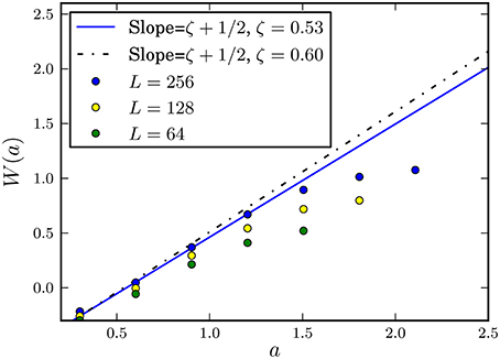
Figure 8. Wavelet analysis of the crack front morphology for different systems sizes (color circles). Results are obtained for stiff systems (i.e., small scale systems) (e = 62.5). The blue line represents the best fit over the obtained points and gives an exponent ζ₋ = 0.53 ± 0.02. The black dashed line refers to the scaling found in the experiments in for small scales: ζ = 0.60 ± 0.05 [12].

It is clear from Figure 8 that the estimated roughness exponent is size dependent. Nevertheless, as the system size increased we observe a convergence of the roughness exponent toward the experimental value represented by the dashed line.

We also performed simulations in the soft regime, which is equivalent to simulating the system on large length scales. We extracted front positions and applied the average wavelet coefficient method to the front morphology. We obtained the roughness exponent by fitting the four largest coefficients for L = 128. This gives: ζ₊ = 0.35 ± 0.01. In Figure 9, we see the wavelet coefficient scaling for this long range regime.

FIGURE 9

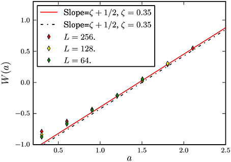
Figure 9. Same as Figure 8 for the soft regime (large scale system) (e = 7.6·10⁻⁶). The experimental value of the roughness exponent for this long range regime is ζ = 0.35 ± 0.05 in agreement with the values obtained from our simulation ζ₊ = 0.35 ± 0.01.

As opposed to the short scale regime, the estimated value of ζ₊ is nearly insensitive to the system size. We also observe that the experimental roughness exponent observed at large length scale [12] is similar to the one we obtained from our simulations.

4.2. Family-Vicsek Scaling

As the fracture front progresses through the system, the memory of the earlier positions fades progressively. We explore this process by creating a differential front h_m with respect to the fracture front at time t₀:

$\begin{array}{cc}{h}_m(x,t)=h(x,t)-h(x,t_0).& (9)\end{array}$

The front width is defined as the root mean square (rms):

$\begin{array}{cc}\sigma (L,t)=\sqrt{{\displaystyle \sum _{x=0}^N{(h_m(x,t,t_0)-{\langle h_m(x,t,t_0)\rangle }_x)}^2}}.& (10)\end{array}$

We chose to use the Family-Vicsek (FV) scaling [37] framework to describe the transient evolution of the differential front:

$\begin{array}{cc}\sigma (t,L)\propto L^{\zeta }f\left(\frac{t}{L^{\kappa }}\right)& (11)\end{array}$

where

$\begin{array}{cc}f(x)=\{\begin{array}{ll}{x}^{\zeta /\kappa }\hfill & x\to 0,\hfill \\ \text{constant}\hfill & x\to \infty .\hfill \end{array}& (12)\end{array}$

and κ is the dynamic exponent.

Since there is no inherent time in the model equations, we have to introduce a a posteriori time definition in order to be able to compare our results to the properties deduced from the experimental setup. We propose to use a simple definition: the average position of the front h_m as a proxy of the time t. Using this time definition, Figures 10 and 11 show the best FV fit for both stiff and soft regimes respectively. It corresponds to the evolution of the rms σ(L, 〈h_m〉) of the front of a system of width L after an average propagation 〈h_m〉. Curves for different system sizes L have been superimposed at best, adjusting the roughness exponent ζ, the dynamic exponent κ and fulfilling the related slope condition: β = ζ/κ.

FIGURE 10

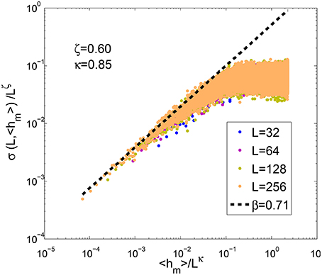
Figure 10. Family-Vicsek scaling for stiff systems i.e., small scale systems (e = 62.5). ζ₋ = 0.6, κ₋ = 0.85 and β₋ = 0.71.

FIGURE 11

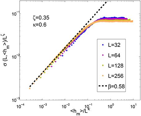
Figure 11. Family-Vicsek scaling for soft systems i.e., large scale systems (e = 7.6·10⁻⁶). ζ₊ = 0.35, κ₊ = 0.6 and β₊ = 0.58.

In both stiff and soft systems, we find the roughness exponent ζ in very good agreement with the results from the average wavelet coefficient method (see Figures 8, 9). The best collapses of the roughness growth curves σ(L, 〈h_m〉) give: κ = 0.85 and β = 0.71 for the stiff regime and κ = 0.6 and β = 0.7 for the soft regime.

4.3. Distribution of Local Velocity

A direct way for studying the dynamics of the fracture propagation is to measure the distribution of the local velocity along the crack front. To obtain this we use the waiting time matrix technique developed by Måløy et al. [11] on experimental data. The waiting time matrix W gives at each sub-squared (i.e., pixel), the time spent by the crack front at this location. This waiting time is measured in our simulations, by identifying the fracture front at each time step (i.e., each broken fiber) and increasing each element of W covered by the crack front by one. After doing this for the entire fracture propagation, we obtain the final estimate of W. From W, we can create the velocity matrix V. Each element of V is indeed the inverse element of W times the discretization length dl¹. This creates a map of the local velocities of the fracture front. Examples of velocity maps are given in Figure 12 for both regimes together with a map at two scales from experimental measurements [31]. It provides a direct visual observation of the pinning of the crack front in our simulation. Comparisons with experimental data show a good agreement and confirm that the stiff regime describes the details of the propagation at small scales and the soft regime at large scales.

FIGURE 12

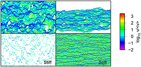
Figure 12. Comparison of the local normalized velocity maps obtained for an experiment at two scales (top): at large scale (top right), and a detail at small scale (top left); and two simulations: in the soft regime (bottom right) and in the stiff regime (bottom left) (bottom). White dots correspond to areas where the local velocity was not measurable, i.e., too fast for the local waiting time method.

Experimentally the distribution of the local velocities v have been found to follow the relation:

$\begin{array}{cc}P(v/\langle v\rangle )\propto {(v/\langle v\rangle )}^{-\eta },\text{for}(v/\langle v\rangle )>1,& (13)\end{array}$

where η = 2.55 ± 0.15 and is found to be a robust feature over many experiments [11, 31, 38].

We see that both regimes (small and large e) produce a power-law decay of the velocity distribution above the average crack velocity consistently with experimental results. The best power law fits for the two regimes, stiff and soft regimes, give η₋ = 2.9 and η₊ = 2.1 respectively.

5. Discussion

To better capture the physical meaning of the controlling parameter e, it is of interest to rewrite e as: $e=d{l}^2/L_f^2·L_f·E$ which reads as: $e=L_f·E/N^2$ where N² is the number of fibers in the system. If one has in mind that L_f·E is the effective stiffness of the elastic medium and N²·1 is the effective stiffness of the set of fibers in parallel (when they are all present and considering a unit stiffness of each fiber), one realizes that e is the ratio of the stiffness of the bulk to the stiffness of the interface: $e=L_f·E/(N^2{k}_f)$ with k_f the stiffness of each fiber. The controlling parameter is then the dimensionless ratio of the two stiffnesses: that of the bulk to that of the interface. When the bulk is very stiff compared to the interface (large e), everything is dominated by the elastic bulk and when the interface is very stiff compared to the bulk, one has a so called soft system.

Using a similar numerical approach, Gjerden et al.[23] obtained advances of the fracture front by introducing a linear gradient in the breaking thresholds with a flat rigid plate. The scaling behavior they found was consistent with a gradient percolation modeling at small scales (large e): ζ₋ = 2/3 and with the contact line model at large scales (small e): ζ₊ = 0.39. In the present problem where there is no gradient in the breaking thresholds but at non-linear displacement loading (a square root profile), we obtained slightly different results. Indeed, the non-linearity may change the scaling exponents in the same way as the introduction of non-linear gradients in the percolation problem [39]. We will pursue this issue in a future publication.

The roughness exponent at small scales with the present model is ζ₋ = 0.60 both from a direct measurement along the fronts using the average wavelet coefficient method and the Family-Vicsek scaling from finite size scaling. This value is very close to the experimental estimate: ζ₋ = 0.60 ± 0.05. At large scales, also both numerical and experimental values match well: ζ₊ = 0.35. Interestingly a recent study [22] reports on a crossover between two scaling regimes of the fracture roughness but invoking a very different mechanism: the porosity of the medium. Below the pore scales, it is argued that the roughness exponent is isotropic with a value close to ζ₋ = 0.8 but at large scale, the roughness exponent is anisotropic with a roughness exponent in the range [0.27 − 0.35]. Actually, it would be of interest to see how the porosity change of the medium is affecting the stiffness of the medium or of the interface and therefore the e modulus.

In Gjerden et al. [24], the dynamical exponent is κ₋ = 1.47 at small scales and κ₊ = 0.75 at large scale. Here we obtained κ₋ = 0.85 and κ₊ = 0.6 which are rather different. Estimates of κ are however not obtained in the same way. In Gjerden et al. [24], they are deduced from a collapse of the front width for different gradients of the strength but not from the finite size scaling. This might explain the discrepancy together with the difference between a linear and a non-linear force perturbation around the fracture tip. κ₋ has been measured in an earlier version of the model [18]: κ₋ = 0.67 and κ₊ with a different approach in Duemmer and Krauth [40]: κ₊ = 0.70.

Comparisons with experimental values of the dynamical exponent κ is rather speculative since there is no experimental measures of κ₋ (e ≫ 1) and κ₊ (e ≪ 1) but of an effective κ for an intermediate e modulus (e ≈ 1). An example of an experimental measure is κ = 1.2 reported by Måløy and Schmittbuhl [41]. An on-going work is devoted to the analysis of the role of the e modulus on the Family-Vicsek scaling and the possible onset of anomalous scaling [42].

The local velocity distribution has also been measured by Gjerden et al. [24] using a linear gradient in the threshold distribution to create the crack front. They followed the same procedure for computing the waiting time matrix as we have done here, and found that, at large scale i.e., for soft systems, the velocity distribution is well fitted by an equation of the form of Equation (13) with an exponent η₊ = 2.53 close to the experimental value.

In Figure 13 we can see the experimental data for the velocity distribution [31], as well as the distribution for the stiff and soft regimes in our model based on a non-linear loading of the system.

FIGURE 13

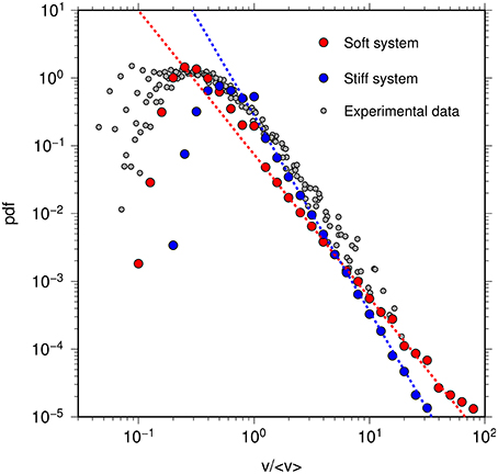
Figure 13. Local velocity distributions from experimental data and stiff and soft models. The best power law fits of the velocity distributions provide estimates of the power law exponents: η₋ = 2.9 (stiff system in red) and η₊ = 2.1 (soft system in blue). For the stiff regime, only velocities in the pinning zones are considered.

6. Conclusions

By introducing a physical loading into the fiber bundle model using a rigid square root shaped plate facing a fully elastic half-space, we obtain very similar results to the experimental values. The square root shape is shown to mimic the elastic opening behind the fracture tip. The scaling of fracture front is shown to exhibit two self-affine regimes using the average wavelet coefficient method (AWC): at small scale (i.e., stiff regime), the roughness exponent is ζ₋ = 0.60 and at large scale (i.e., soft regime), ζ₊ = 0.35 very similarly to the experimental measures reported by Santucci et al. [12] (ζ₋ = 0.60 and ζ₊ = 0.35). The cross-over between both regimes is controlled by the reduced e modulus which is shown to be related to the ratio of the stiffness of the bulk and the stiffness of the interface.

Transient roughening is studied in the Family-Viscek scaling framework. We measured the evolution of the root mean square of the fracture front roughness from a reference front as a function of the average position of the front. We obtained good collapses of the roughness growth for different system sizes using a roughness exponent ζ consistent with the direct measurements and a dynamical exponent κ. For the small scale regime, i.e., the stiff regime, we measured: κ₋ = 0.85. For the large scale regime, i.e., the soft regime, we estimated: κ₊ = 0.60. Both values are consistent with the independently measured β = ζ/κ: β₋ = 0.71 for the stiff regime and β₊ = 0.58 for the soft regime. Our roughness exponents are close to that of Gjerden et al. [23]. The Gjerden analysis for the hard case was based on the assumption that the problem was in the universality class of ordinary percolation. The dynamical exponents κ are on the contrary rather different which is expected to be related to the differences in loading: linear gradient of the fiber strength vs. non-linear imposed displacement. The dynamical exponent seems accordingly more sensitive to the difference in the models. Comparisons with experiments of the dynamical exponent is difficult since there is no measure of the dynamical exponents for the extreme case e ≪ 1 and e ≫ 1 but only for intermediate cases. An interesting forthcoming study will deal with the effect of the e modulus on the dynamical scaling of the fracture front.

We also compared the local velocity distribution of our model to the distribution found in experiments. Both are consistent with a power law distribution: P(v/〈v〉)∝(v/〈v〉)^−η with η_exp = 2.55 for the experiment, η₋ = 2.9 for the stiff regime and η₊ = 2.1 for the soft regime.

Author Contributions

AS did the programming, produced data, some analysis and a first draft. OL did experimental work, produced data and some analysis. He also updated the text. JS did data analysis and updated the manuscript. AH did data analysis and updated the manuscript.

Conflict of Interest Statement

The authors declare that the research was conducted in the absence of any commercial or financial relationships that could be construed as a potential conflict of interest.

The reviewer JB and handling Editor declared a current collaboration and the handling Editor states that the process nevertheless met the standards of a fair and objective review.

Acknowledgments

We thank K. S. Gjerden and K. J. Måløy for insightful discussions and A. Steyer for technical support for the experimental work. We furthermore acknowledge support from ANR SUPNAF, Labex G-EAU-THERMIE PROFONDE (grant no. ANR-11-LABX-0050) and the Norwegian Research Council through grant no. 1999770.

Footnotes

1. ^When W = 0, we replaced the inverse by 9999.9999 in order to ensure that they are indeed treated as large velocities by the program.

References

1. Alava, MJ, Nukala, PK, and Zapperi, S. Statistical models of fracture. Adv Phys. (2006) 55:349–476. doi: 10.1080/00018730300741518

CrossRef Full Text | Google Scholar

2. Bonamy, D, and Bouchaud, E. Failure of heterogeneous materials: a dynamic phase transition? Phys Rep. (2011) 498:1–44. doi: 10.1016/j.physrep.2010.07.006

CrossRef Full Text | Google Scholar

3. Anderson, TL, and Anderson, T. Fracture Mechanics: Fundamentals and Applications. Boca Raton, FL: CRC Press (2005).

Google Scholar

4. Scholz, CH. The Mechanics of Earthquakes and Faulting. Cambridge: Cambridge University Press (2002).

Google Scholar

5. Bouchaud, E. Scaling properties of cracks. J Phys. (1997) 9:4319. doi: 10.1088/0953-8984/9/21/002

PubMed Abstract | CrossRef Full Text | Google Scholar

6. Mandelbrot, BB, Passoja, DE, and Paullay, AJ. Fractal character of fracture surfaces of metals. Nature (1984) 308:721–2. doi: 10.1038/308721a0

CrossRef Full Text | Google Scholar

7. Barabási, AL. Fractal Concepts in Surface Growth. Cambridge: Cambridge University Press (1995).

Google Scholar

8. Schmittbuhl, J, and Måløy, KJ. Direct observation of a self-affine crack propagation. Phys Rev Lett. (1997) 78:3888. doi: 10.1103/PhysRevLett.78.3888

CrossRef Full Text | Google Scholar

9. Delaplace, A, Schmittbuhl, J, and Måløy, KJ. High resolution description of a crack front in an heterogeneous plexiglas block. Phys Rev E (1999) 60:1337–43. doi: 10.1103/PhysRevE.60.1337

PubMed Abstract | CrossRef Full Text | Google Scholar

10. Måløy, KJ, and Schmittbuhl, J. Dynamical events during slow crack propagation. Phys Rev Lett. (2001) 87:105502. doi: 10.1103/PhysRevLett.87.105502

PubMed Abstract | CrossRef Full Text | Google Scholar

11. Måløy, KJ, Santucci, S, Schmittbuhl, J, and Toussaint, R. Local waiting time fluctuations along a randomly pinned crack front. Phys Rev Lett. (2006) 96:045501. doi: 10.1103/PhysRevLett.96.045501

PubMed Abstract | CrossRef Full Text | Google Scholar

12. Santucci, S, Grob, M, Toussaint, R, Schmittbuhl, J, Hansen, A, and Maløy, KJ. Fracture roughness scaling: a case study on planar cracks. Europhys Lett. (2010) 92:44001. doi: 10.1209/0295-5075/92/44001

CrossRef Full Text | Google Scholar

13. Sahimi, M. Non-linear and non-local transport processes in heterogeneous media: from long-range correlated percolation to fracture and materials breakdown. Phys Rep. (1998) 306:213–395. doi: 10.1016/S0370-1573(98)00024-6

CrossRef Full Text | Google Scholar

14. Chen, K, Bak, P, and Obukhov, S. Self-organized criticality in a crack-propagation model of earthquakes. Phys Rev A (1991) 43:625. doi: 10.1103/PhysRevA.43.625

PubMed Abstract | CrossRef Full Text | Google Scholar

15. Dickman, R, Muñoz, MA, Vespignani, A, and Zapperi, S. Paths to self-organized criticality. Brazil J Phys. (2000) 30:27–41. doi: 10.1590/S0103-97332000000100004

CrossRef Full Text | Google Scholar

16. Schmittbuhl, J, Roux, S, Vilotte, JP, and Måløy, KJ. Interfacial crack pinning: effect of nonlocal interactions. Phys Rev Lett. (1995) 74:1787. doi: 10.1103/PhysRevLett.74.1787

PubMed Abstract | CrossRef Full Text | Google Scholar

17. Rosso, A, and Krauth, W. Roughness at the depinning threshold for a long-range elastic string. Phys Rev E (2002) 65:025101. doi: 10.1103/PhysRevE.65.025101

PubMed Abstract | CrossRef Full Text | Google Scholar

18. Schmittbuhl, J, Hansen, A, and Batrouni, GG. Roughness of interfacial crack fronts: stress-weighted percolation in the damage zone. Phys. Rev. Lett. (2003) 90:045505. doi: 10.1103/PhysRevLett.90.045505

PubMed Abstract | CrossRef Full Text | Google Scholar

19. Ponson, L, Bonamy, D, and Bouchaud, E. Two-dimensional scaling properties of experimental fracture surfaces. Phys Rev Lett. (2006) 96:035506. doi: 10.1103/PhysRevLett.96.035506

PubMed Abstract | CrossRef Full Text | Google Scholar

20. Ponson, L, Auradou, H, Vié, P, and Hulin, JP. Low self-affine exponents of fractured glass ceramics surfaces. Phys Rev Lett. (2006) 97:125501. doi: 10.1103/PhysRevLett.97.125501

PubMed Abstract | CrossRef Full Text | Google Scholar

21. Bonamy, D, Ponson, L, Prades, S, Bouchaud, E, and Guillot, C. Scaling exponents for fracture surfaces in homogeneous glass and glassy ceramics. Phys Rev Lett. (2006) 97:135504. doi: 10.1103/PhysRevLett.97.135504

PubMed Abstract | CrossRef Full Text

22. Cambonie, T, Bares, J, Hattali, M, Bonamy, D, Lazarus, V, and Auradou, H. Effect of the porosity on the fracture surface roughness of sintered materials: from anisotropic to isotropic self-affine scaling. Phys Rev E (2015) 91:012406. doi: 10.1103/PhysRevE.91.012406

PubMed Abstract | CrossRef Full Text | Google Scholar

23. Gjerden, KS, Stormo, A, and Hansen, A. Universality classes in constrained crack growth. Phys Rev Lett. (2013) 111:135502. doi: 10.1103/PhysRevLett.111.135502

PubMed Abstract | CrossRef Full Text | Google Scholar

24. Gjerden, KS, Stormo, A, and Hansen, A. Local dynamics of a randomly pinned crack front: a numerical study. Front Phys. (2014) 2:66. doi: 10.3389/fphy.2014.00066

CrossRef Full Text | Google Scholar

25. Pradhan, S, Hansen, A, and Chakrabarti, BK. Failure processes in elastci fiber bundles. Rev Mod Phys. (2010) 82:499. doi: 10.1103/RevModPhys.82.499

PubMed Abstract | CrossRef Full Text

26. Hansen, A, Hemmer, PC, and Pradhan, S. The Fiber Bundle Model. Weinheim: Wiley-VCH (2015).

Google Scholar

27. Batrouni, GG, Hansen, A, and Schmittbuhl, J. Heterogeneous interfacial failure between two elastic blocks. Phys. Rev E (2002) 65:036126. doi: 10.1103/PhysRevE.65.036126

PubMed Abstract | CrossRef Full Text | Google Scholar

28. Delaplace, A, Schmittbuhl, J, and Måløy, KJ. High resolution description of a crack front in a heterogeneous Plexiglas block. Phys Rev E (1999) 60:1337. doi: 10.1103/PhysRevE.60.1337

PubMed Abstract | CrossRef Full Text | Google Scholar

29. Lengliné, O, Toussaint, R, Schmittbuhl, J, Elkhoury, JE, Ampuero, JP, Tallakstad, KT, et, al. Average crack-front velocity during subcritical fracture propagation in a heterogeneous medium. Phys Rev E (2011) 84:036104. doi: 10.1103/PhysRevE.84.036104

PubMed Abstract | CrossRef Full Text

30. Lengliné, O, Schmittbuhl, J, Elkhoury, JE, Ampuero, JP, Toussaint, R, and Måløy, KJ. Down-scaling of the fracture energy during brittle creep experiments. (2011) J Geophys Res. 116:B08215. doi: 10.1029/2010JB008059

CrossRef Full Text

31. Lengliné, O, Elkhoury, JE, Daniel, G, Schmittbuhl, J, Toussaint, R, Ampuero, JP, et, al. Interplay of seismic and aseismic deformations during earthquake swarms: an experimental approach. Earth Planet Sci Lett. (2012) 331–332:215–23. doi: 10.1016/j.epsl.2012.03.022

CrossRef Full Text

32. Love, AEH. The stress produced in a semi-infinite solid by pressure on part of the boundary. Philos Trans R Soc London Ser A (1929) 228:377–420.

Google Scholar

33. Rice, JR. First-order variation in elastic fields due to variation in location of a planar crack front. J Appl Mech. (1985) 52:571–9. doi: 10.1115/1.3169103

CrossRef Full Text | Google Scholar

34. Gjerden, KS, Stormo, A, and Hansen, A. A model for stable interfacial crack growth. In: Journal of Physics: Conference Series. Vol. 402 Bristol, UK: IOP Publishing (2012). p. 012039

Google Scholar

35. Stormo, A, Gjerden, KJ, and Hansen, A. Onset of localization in heterogeneous interfacial failure. Phys Rev E (2012) 86:025101. doi: 10.1103/PhysRevE.86.025101

PubMed Abstract | CrossRef Full Text | Google Scholar

36. Simonsen, I, Hansen, A, and Nes, OM. Determination of the Hurst exponent by use of wavelet transforms. Phys Rev E (1998) 58:2779. doi: 10.1103/PhysRevE.58.2779

CrossRef Full Text | Google Scholar

37. Family, F, and Vicsek, T. Scaling of the active zone in the Eden process on percolation networks and the ballistic deposition model. J Phys A Math Gen. (1985) 18:L75. doi: 10.1088/0305-4470/18/2/005

CrossRef Full Text | Google Scholar

38. Tallakstad, KT, Toussaint, R, Santucci, S, Schmittbuhl, J, and Måløy, KJ. Local dynamics of a randomly pinned crack front during creep and forced propagation: an experimental study. Phys Rev E (2011) 83:046108. doi: 10.1103/PhysRevE.83.046108

PubMed Abstract | CrossRef Full Text | Google Scholar

39. Hansen, A, and Schmittbuhl, J. Origin of the universal roughness exponent of brittle fracture surfaces: stress-weighted percolation on the damage zone. Phys Rev Lett. (2003) 90:045504. doi: 10.1103/PhysRevLett.90.045504

PubMed Abstract | CrossRef Full Text | Google Scholar

40. Duemmer, O, and Krauth, W. Depinning exponents of the driven long-range elastic string. J Stat Mech Theory Exp. (2007) 2007:P01019. doi: 10.1088/1742-5468/2007/01/P01019

CrossRef Full Text | Google Scholar

41. Måløy, KJ, and Schmittbuhl, J. Dynamical event during slow crack propagation. Phys Rev Lett. (2001) 87:105502. doi: 10.1103/PhysRevLett.87.105502

PubMed Abstract | CrossRef Full Text | Google Scholar

42. López, JM, and Schmittbuhl, J. Anomalous scaling of fracture surfaces. Phys Rev E (1998) 57:6405.

Google Scholar