On the Role of Fluctuations in the Modeling of Complex Systems

1. Introduction

One generic type of question a scientist has to face is to understand and explain the behavior of a given system found in nature. This type of problems occur in different fields of physics, chemistry, biology, ecology but also in economics, and sociology. Often the problem is of interdisciplinary nature and has a complex character.

A frequent approach to study such a situation is to introduce a model describing the properties of a system using a set of variables considered to be relevant. However, it is not always obvious to decide what are the relevant variables, because there are several levels of description of reality.

As written by Einstein, “Everything should be made as simple as possible, but not simpler” [1]. Thus, one would like to be able to decide which is the simpler, yet acceptable, model before starting a detailed investigation.

Let us consider, to illustrate this point, the case of a simple fluid. We would like to propose a model explaining and making some predictions concerning the flow of such a liquid in a particular situation (boundary conditions, external forces…). How to model such a fluid? At a macroscopic level, the relevant observables are the so-called hydrodynamic variables, namely the local density, the velocity field, and the pressure [2]. A simple approach is to write hydrodynamic equations based on the laws of classical mechanics and the conservation laws in the problem [3]. One ends up with partial differential equations (continuity and Navier-Stokes equations) which could be in some simple cases solved analytically or generally integrated numerically. But at a different level, one could argue that one knows that a fluid is nothing but a family of interacting molecules and that one knows how these molecules interact among each other. This may be a better description of the reality than the previous one. It is a bottom-up approach and the problem is then how to extract the properties of the hydrodynamic variables from this microscopic modeling. One way is to develop approximative analytical methods, like the Boltzmann formalism [2], another way is to integrate numerically the microscopic equations of motion for the interacting molecules and average out to obtain the hydrodynamic fields. However, this could be a tremendous task in view of the complex form of the inter-molecular interactions. This lead us to ask the following question: how important are the details of the molecular interactions in the determination of the generic form of the equations of motion for the hydrodynamic variables? Or formulated in a different way, is it possible to define a simpler model in which the molecules are replaced by fictitious agents interacting in a simple way, but not too simple, which respect the basic conservations laws of the system? This is indeed possible and realized by the cellular automata or lattice gas approaches which is now widely used in fluid mechanics [4]. The generic form of the equations of motion for the hydrodynamic variables is not affected by this simplification, however the values of the transport coefficients, like the viscosity, depend on the particular approximation used. It turns out that the three different approaches sketched above lead fortunately to the same conclusions for the dynamics of our fluid. However, depending on the particular problem one has to solve, the macroscopic approach and the lattice-gas one could have a drastically different cost.

Sometimes however predictions provided by different levels of description could be totally different. Let us consider two limiting cases: the so-called mean-field approximation where the dynamics is described in terms of spatially averaged quantities and the microscopic approach in which the local properties of the system are taken into account. These two cases differ by the absence or presence of local fluctuations of the relevant variables. The properties predicted by these two different approaches may be drastically different.

It is true that mean-field like approximations are often easy to perform while microscopic calculations can be very complicated due to different reasons, one being the large number of control parameters entering into the model. Thus, the cost of a microscopic approach may be tremendously higher than the cost of a mean-field like approach and it is tempting to restrict oneself to such a simple approach. However, in some cases the fluctuations play a crucial role. We realized that a large body of research papers, mainly in biological or ecological fields, are based on simple mean-field like approximation and that, when discussing with the authors, they often do not understand why fluctuations should enter into their model. Thus, the goal of this paper is twofold, first to illustrate the importance of the fluctuations in a self-contained and pedagogical way, by revisiting two different classes of problems where thorough investigations have been conducted on the role played by the fluctuations.

The first one is equilibrium statistical physics (Section 2). To be explicit we shall discuss the so-called Ising model, describing the equilibrium phase transition between the paramagnetic and ferromagnetic phases of a spin system [5]. This model is a paradigm for equilibrium statistical mechanics and more than 40 thousand research papers have been devoted to this model. This will illustrate, in a pedagogical way what effects fluctuations can possibly have and the possibility to establish a criterion to decide on the relevance of the fluctuations.

The second domain we consider is non-equilibrium statistical physics (Section 3) and we shall concentrate on a class of problems having numerous application in physical-chemistry [6], biology [7], and sociology [8], namely reaction-diffusion systems. New difficulties related to fluctuations in the initial conditions will be discussed and new methodological tools introduced to understand the role played by fluctuations. No criterion concerning the validity of mean-field like approximation can be established.

In Section 4, as a new example of the role of approximation adopted, we present our original research on the dynamics of population of annual plants which are competing among themselves for just one resource (water) through a stochastic dynamics [9]. During each year, they are surviving or dying according to the availability of the resource and their tolerance to lack or surplus of water. At the end of the year, the alive plants produce seeds which are dispersed in their neighborhood and all plants die. At the beginning of a next year, seeds germinate and the yearly cycle starts again. At the crudest level, one considers the average plant density with no spatial dependence, this is the mean-field level. At the opposite end, the dynamics is described by an Individually Based Model (IBM) [10, 11], in which the dynamics of each single plant is followed separately. Which is the best description? Depending on the observable considered, sometimes the two different approaches agree, sometimes they totally disagree. It is difficult in this case to formulate a first principle criterion telling whether much simpler mean-field approximation is good enough, or if we have to turn to the IBM. To the best of our knowledge there is no such a criterion in biological literature neither a detailed study of the problem.

Finally, some conclusions are drawn in Section 5.

2. Equilibrium Statistical Physics

Some materials when cooled down exhibit a phase transition from a paramagnetic phase at high temperature to a ferromagnetic phase at low temperature. This transition takes place at a well defined temperature, the critical or Curie temperature T_c which depends on the material. The low temperature phase is characterized by the presence of a spontaneous magnetization per particle m(T) which depends on the temperature. At zero temperature T = 0, the magnetization is maximal and decreases with increasing T. If m(T) → 0 as T → T_c continuously, one speaks of a “continuous phase transition” while if m(T) → m₀ ≠ 0 as $T\to T_c^{-}$ while m(T) = 0 for T > T_c, one speaks of a “discontinuous transition.” The continuous phase transition is then associated with a spontaneous symmetry breaking and the spontaneous magnetization is called the “order parameter” of the transition. Beside the magnetization m(T) several other physical quantities, like for example the magnetic susceptibility or the specific heat exhibit, near T_c a power law behavior of the type:

$\begin{array}{ll}X(t)~{\mid t\mid }^{-x},& (1)\end{array}$

where t = (T − T_c)/T_c is the so-called reduced temperature and x is the critical exponent associated to the observable X.

Let us consider the simplest case in which the magnetization can be aligned only along a particular direction that we may call z. Thus, the magnetization is a scalar quantity.

How to model such a system? A simple way is to suppose that at a mesoscopic level, the atoms constituting the material are carrying a classical spin variable s_i = ±1, where i denotes the position of the spin and corresponds to a site on a d-dimensional hypercubic lattice for example. The spins are interacting among themselves and with a heat bath at temperature T. The equilibrium properties of the system can then be described in the formalism of equilibrium statistical physics and particularly by the canonical ensemble. The Hamiltonian, describing the energy of the spins system is

$\begin{array}{ll}H=-{\displaystyle \sum _{i,j}}{J}_{i,j}{s}_i{s}_j-h{\displaystyle \sum _i}{s}_i,& (2)\end{array}$

where the sums run over all the sites 1, …, N of the lattice, and h is an external magnetic field. This model is called the Ising model [12]. In the simplest case when only the nearest neighbors interact, J_{i, j} = J if i and j are nearest neighbor and zero otherwise. Moreover, if J > 0 and when h = 0 and T = 0, all the spins are aligned in the same direction. The ground states are then ferromagnetic and one speaks of ferromagnetic like interactions.

The physical observables are directly related to the canonical partition function

$\begin{array}{ll}Z(T,N)=Tr\left[\text{exp}-(\beta H)\right],& (3)\end{array}$

where Tr means the sum over the 2^N possible spin configurations of the system and $\beta ={\left[k_{B}T\right]}^{-1}$, where k_B is the Boltzmann constant. From Z, all thermodynamic quantities can be obtained. The free energy is

$\begin{array}{ll}F(T,N)=-k_{B}TlogZ(T,N),& (4)\end{array}$

the total magnetization

$\begin{array}{ll}M(T,h)=\frac{\partial }{\partial (\beta h)}logZ(T,N)& (5)\end{array}$

and the magnetization per spin in the thermodynamic limit is thus

$\begin{array}{ll}m(T,h)={\displaystyle \underset{N\to \infty }{lim}}{N}^{-1}M(T,h).& (6)\end{array}$

Finally, the zero field specific heat is

$\begin{array}{ll}C(T)=-T\frac{{\partial }^{2}f(T)}{\partial T^2}.& (7)\end{array}$

where f(T) is the free energy per spin. The difficulty is to obtain an analytic solution of the partition function in the thermodynamic limit N → ∞. For a one dimensional system, the transfer matrix method allows one to solve this problem easily. As shown by Ising in 1925, in this case the critical temperature is zero, i.e., there is no phase transition [12]. For dimensions larger than 1, the computation of Z is a formidable task [13]. In d = 2, h = 0, and nearest neighbors interactions, Onsager in a seminal paper [14] showed that there is a transition for T_c given by sinh(2J/(k_BT_c)) = 1. Moreover, this transition is continuous and the spontaneous magnetization behaves, near the critical point, as

$\begin{array}{ll}m(T)=\{\begin{array}{ll}{[1-{(2\text{sinh }2\nu )}^{-4}]}^{1/8}~t^{1/8}\hfill & \text{if }t<0,\hfill \\ 0\hfill & \text{if }t>0,\hfill \end{array}& (8)\end{array}$

where ν = J/(k_BT). The specific heat C(T) has a symmetrical logarithmic divergence at the critical point ν_c, i.e.,

$\begin{array}{ll}C(T)~log(|\nu -{\nu }_c|).& (9)\end{array}$

The behavior of the physical quantities in the vicinity of the critical point has the form of power laws and it is usual to write

$\begin{array}{ll}m(T)~\{\begin{array}{ll}|t{|}^{\beta }\hfill & \text{if }t<0,\hfill \\ 0\hfill & \text{if }t>0,\hfill \end{array}& (10)\end{array}$

and

$\begin{array}{ll}C(T)~{\left|t\right|}^{-\alpha }& (11)\end{array}$

for t → 0. The exponents β and α are called the critical exponents (Note that the symbol β has two different meanings, the inverse temperature as in Equation(3) and the critical exponent of the magnetization as in Equation (10). This is the standard notation for both quantities and there should be no ambiguities when reading the text). For d = 2, the exponents have the values α = 0 and β = 1/8 which are in agreement with experimental data. Moreover, the spatial decay of the two-spins correlation function is exponential with a characteristic length ξ(t) which diverges as a power law of the reduced temperature as T → T_c.

There are still no analytical solutions for d > 2. However, different numerical approaches, like the Monte-Carlo method [15] show that there is a continuous transition for all dimensions d ≥ 2 in zero external field.

The main reason for which it is so difficult to compute the canonical partition function Z(T, N) is the presence of the quadratic terms s_is_j. A simpler way to model the ferromagnetic interactions among the spins consists in assuming that the spin s_i feels the influence of the neighbor spins through an effective or average field. This is the basic idea in the so called mean-field or Curie Weiss theory [16]. Technically it can be realized as follows. Let us write each spin variable s_i as an ensemble average part 〈s_i〉 plus a fluctuating part δs_i. Then the quadratic term can be written as

$\begin{array}{ll}{s}_i{s}_j=\langle s_i\rangle \langle s_j\rangle +\langle s_i\rangle \delta s_j+\langle s_j\rangle \delta s_i+\delta s_i\delta s_j& (12)\end{array}$

The mean-field approximation consist in neglecting the last term quadratic in the fluctuations. Moreover, 〈s_i〉 = m by translational invariance. Thus, the initial Ising Hamiltonian becomes very simple, H → H_mf and

$\begin{array}{ll}{H}_{mf}=12NzJ{m}^2-h_{mf}{\displaystyle \sum _{i=1}^N}{s}_i,& (13)\end{array}$

where z is the coordination number of the lattice (z = 2^d for a d-dimensional hypercubic lattice) and

$\begin{array}{ll}{h}_{mf}=Jzm+h.& (14)\end{array}$

One is left with a very simple problem as the mean-field Hamiltonian is the sum of one spin Hamiltonians. The magnetization per spin obeys the following relation

$\begin{array}{ll}m(T)=tanh\left[{(k_{B}T)}^{-1}(Jzm(T)+h)\right].& (15)\end{array}$

In zero external field, the spontaneous magnetization is zero above the critical temperature $T_c^{mf}=Jz/k_B$ and

$\begin{array}{ll}m(T)~\{\begin{array}{cc}|t{|}^{\beta }& \mathrm{\text{if }}t<0,\\ 0& \mathrm{\text{if }}t>0,\end{array}& (16)\end{array}$

where now $t=(T-T_c^{mf})/(T_c^{mf})$ and β = 1/2. The specific heat (in zero external field) exhibits a discontinuity at $T_c^{mf}$

$\begin{array}{ll}C(T)~\{\begin{array}{ll}3/2k_B& \mathrm{\text{if }}T={\displaystyle {lim}_{ϵ\to 0}}{T}_c^{mf}-ϵ,\\ 0& \mathrm{\text{if }}T>T_c^{mf}.\end{array}& (17)\end{array}$

One notes that the predictions of the mean-field approach are quite different from the ones obtained when the trace over all fluctuations has been accounted for. For example, the mean-field approach predicts a phase transition with a finite critical temperature in all dimensions, while we know that in one dimension T_c = 0. In two dimensions, the behavior of the spontaneous magnetizations is quite different (different critical exponents) and the specific heat has a logarithmic divergence at T_c in one case and a discontinuity in the other case. Thus clearly, the mean-field model which does not take the fluctuations into account is too simple a model to describe correctly the reality. However, in view of its great simplicity it would be useful to know if its prediction are still valid under some conditions. We shall address this problem later.

Before going to this point, we would like to review a different approach which allows us to obtain the mean-field results starting from a microscopic model without neglecting the fluctuations in a brute force manner. This is the Ising model with long range interactions [17]. This approach is not well known outside the community of statistical physicists and, as we shall see later, turns out to be quite useful when applied to ecological or biological problems for which the dynamics involve pair of sites separated by arbitrarily large distances.

Let us return to the Ising Hamiltonian (see Equation 2) but now, we suppose that J_{i, j} couple all the pairs of spins. The interactions have to be properly normalized to guarantee that the thermodynamic limit exists. Thus, the Hamiltonian reads:

$\begin{array}{ll}H=-\frac{J_0}{2N}{\displaystyle \sum _{1\le i<j\le N}}{s}_i{s}_j-h{\displaystyle \sum _{1\le i\le N}}{s}_i& (18)\end{array}$

as s_i = ±1, the canonical partition function can be written as

$\begin{array}{ll}Z(T,N)=\exp (-\nu /2)Tr\exp [\frac{\nu }{2N}{({\displaystyle \sum _{1\le i<j\le N}{s}_i})}^2+b{\displaystyle \sum _{1\le i\le N}{s}_i}],& (19)\end{array}$

where ν = βJ₀ and b = βh. This form still causes problems because all the spins remain coupled by the term quadratic in s_i. However, the spins can be decoupled by using the Hubbard-Stratonovitch [18] transformation:

$\begin{array}{ll}exp\left(\frac{a}{2}\right)={(2\pi )}^{-1/2}{\displaystyle {\int }_{\infty }^{\infty }}exp(-x^2/2+\sqrt{a}x)dx& (20)\end{array}$

with

$\begin{array}{ll}{a}^{1/2}={(\nu /N)}^{1/2}{\displaystyle \sum _{1\le i\le N}}{s}_i.& (21)\end{array}$

Thus, the trace on the 2^N spin configurations decouples and one ends up with the partition function expressed in terms of a very complicated integral, namely

$\begin{array}{l}Z(T,N)={(2\pi )}^{-1/2}\exp (-\nu /2){\displaystyle {\int }_{-\infty }^{\infty }d}x\exp (-x^2/2)\\ {[2\text{ cosh}(x{(\nu /N)}^{1/2}+b)]}^N.& (22)\end{array}$

The computation of this last integral seems to be hopeless. However, in the thermodynamic limit N → ∞, this integral can be computed using the saddle point method. From the value of Z, the free energy density follows and thus the magnetization per spin which obeys the relation

$\begin{array}{ll}m(t,h)=tanh(\nu m+b).& (23)\end{array}$

The critical temperature in this case is given by ν_c = 1, thus k_BT_c = J₀. We thus recover the results of the mean-field or Curie Weiss theory [16]. By forcing all the spins to interact, one introduces some rigidity among them and it is not really surprising that the fluctuations are suppressed.

We can now return to the generic question of when neglecting the fluctuations is a reasonable approximation. This criterion is known as the Ginzburg-Landau criterion [19]. The idea leading to this criterion is quite simple. Let us consider a physical quantity as for example the specific heat C(T). As we have seen above for the 2-d Ising model, near the critical temperature, the mean-field approximation gives for the specific heat C(T) = C₁(T), while the exact theory leads to a logarithmic singularity. Thus C(T) is composed of two parts C(T) = C₁(T) + C₂(T) where C₂(T) is the contribution coming from the fluctuations. Let us call

$\begin{array}{ll}{R}_{GL}=\frac{C_2(T)}{C_1(T)}& (24)\end{array}$

the Ginzburg-Landau parameter. If R_GL ≪ 1, the fluctuations are negligible and the mean-field approximation is acceptable. If R_GL ≫ 1, the fluctuations play a very important role. How to compute R_GL? As we have seen above, in the vicinity of the critical point of a continuous phase transition, the correlation length diverges and cooperative phenomena are very strong. This indicates that the properties of the system are insensitive to the microscopic details. Moreover, the transition is associated with a continuous symmetry breaking characterized by an order parameter. These facts lead Ginzburg and Landau to formulate a phenomenological model [19] capable of describing a wide class of phase transitions. We shall not describe the Ginzburg-Landau theory in great detail, but only recall the main ideas. The key quantity is the order parameter. For simplicity, we restrict ourselves to a scalar order parameter $m(\overrightarrow{r})$ which may vary continuously in a d-dimensional space (note however that the order parameter could be a vector or a tensor). The Ginzburg-Landau Hamiltonian H_GL is then the spatial integral of a polynomial expression of $m(\overrightarrow{r})$ containing powers and gradients. The polynomial should reflects the symmetries of the problem. The Ginzburg-Landau partition function is given by a functional integral over the possible realizations $m(\overrightarrow{r})$ of the Boltzmann factor exp(−βH_GL). The computation of this functional integral is not possible without some approximations. The crudest approximation consists in retaining $m(\overrightarrow{r})$ which minimizes H_GL. This is simply the solution obtained above in the mean-field approximation, m_mf. The next approximation consists in keeping the fluctuations $\delta m(\overrightarrow{r})=m(\overrightarrow{r})-m_{mf}$ to the lowest order. This defines the Gaussian model from which the contribution to the specific heat related to the fluctuations C₂(T) can be computed. Thus, R_GL can be written as

$\begin{array}{ll}{R}_{GL}~{\left|{\zeta }_{T}t\right|}^{(d-4)/2},& (25)\end{array}$

where ζ_T is the so-called Ginzburg parameter which value depends on the system studied. First one notes that the dimension d = d_c = 4, called the upper critical dimension, plays a particular role. For a system in dimension d > 4 the mean-field theory is essentially correct. However, when d < 4 and t small enough, the fluctuations play a very important role. This defines the critical region of width given by |ζ_Tt| = 1. Inside the critical region the fluctuations are important, outside of it they can be neglected. As t increases when d < 4 the role of the fluctuation decreases and a mean-field approximation is again reasonable.

In summary, the fluctuations play a crucial role in many respects. They are responsible for the fact that below d = d_l = 2 there is no ordered phase (d_l is called the lower critical dimension). For d > d_u = 4 the mean-field approximation is essentially correct. For 4 > d > 2 a simple mean-field approach is correct outside the critical region, but incorrect near the critical temperature.

3. Non-Equilibrium Statistical Physics

Reaction-diffusion problems are simple examples of non-equilibrium systems. The understanding of the kinetics of reaction-diffusion problems is an important issue because potential applications of these ideas in different fields, as physics, chemistry, biology or sociology are numerous. For the sake of simplicity, we shall restrict ourselves in this discussion to some simple cases. However, a large literature is devoted to more complicated situations [20, 21].

3.1. Reaction among Two Species with Homogeneous Initial Conditions

Let us consider a simple model in which two species A and B are homogeneously distributed in a d-dimensional box. The two species diffuse independently and react when they meet to form an inert species: A + B → inert. Given some initial uniform densities ρ_A(0) and ρ_B(0) such that ρ_A(0) = ρ_B(0), what are the long term behaviors ρ_A(t) = ρ_B(t) = ρ(t)? This situation could for example model the recombination of electrons and holes or the annihilation of topological defects in solid-state physics. In the simplest approximation, one could assume that the agents are stirred rapidly and then the law of mass action [22] can be applied. Thus

$\begin{array}{ll}\frac{d{\rho }_A(t)}{dt}=\frac{d{\rho }_B(t)}{dt}=-k{\rho }_A(t){\rho }_B(t),& (26)\end{array}$

where k is the reaction rate. In the long time limit, the solution is

$\begin{array}{ll}\rho (t)~\frac{1}{kt}.& (27)\end{array}$

Thus, ρ(t) decreases with time as a power law and the dimension does not enter explicitly in this equation. This derivation corresponds to the mean-field approximation and should be valid only when the species are well stirred. If there is no stirring the species have to find each other by diffusion and thus one expects that the dynamics will be slower and depend on the dimensionality d of the system. Indeed, taking the diffusion into account, the dynamics for the local concentrations is given by the equations

$\begin{array}{ll}\frac{d{\rho }_A(\overrightarrow{r},t)}{dt}=D_A{\nabla }^2{\rho }_A(\overrightarrow{r},t)-k{\rho }_A(\overrightarrow{r},t){\rho }_B(\overrightarrow{r},t),& (28)\end{array}$

and

$\begin{array}{ll}\frac{d{\rho }_B(\overrightarrow{r},t)}{dt}=D_B{\nabla }^2{\rho }_B(\overrightarrow{r},t)-k{\rho }_A(\overrightarrow{r},t){\rho }_B(\overrightarrow{r},t),& (29)\end{array}$

where D_A and D_B are respectively the diffusion coefficients of the A and B agents. Then, if D_A = D_B = D, as noticed by Toussaint and Wilczek [23] the local density differences ${\rho }_A(\overrightarrow{r},t)-{\rho }_B(\overrightarrow{r},t)$ obeys a diffusion equation. As a consequence, central limit arguments led Toussaint and Wilczek to conclude that number of agents decays as ${\rho }_A,{\rho }_B~{(Dt)}^{-d/4}$.

This behavior can be explained by a simple and elegant heuristic argument [24]. Let us consider a box of volume V = ℓ^d inside the system. At time t = 0 the quantity of species A in this volume fluctuates and is $N_A={\rho }_A(0){\ell }^d\pm \sqrt{{\rho }_A(0){\ell }^d}$. After a time ℓ²/D, where D is the diffusion constant (we suppose that D_A = D_B = D), the agents in V will have time to be mixed completely and react, leaving only the residual fluctuations. Residual A in this domain is $\sqrt{{\rho }_A(0){\ell }^d}$ with density $\sqrt{{\rho }_A(0){\ell }^{-d}}$. The system is then formed by a collection of alternating A rich and B rich domains of typical size ℓ ~ (Dt)^1/2 and the global density is then $\rho (t)~\sqrt{\rho (0)}{(Dt)}^{-d/4}$. This decay with the exponent d/4 (for d ≤ 4) is in agreement with the experimental data and the predictions of theoretical models taking the fluctuations into account. When d > 4 the slowest decay is given by the mean-field solution. Thus, in general ρ(t) ~ t^−z with z = min(d/4, 1). Here again, an upper critical dimension d_u = 4 enters into the kinetics of the problem. Neglecting the fluctuations when d < 4 leads to completely wrong conclusions.

Thus, models which are able to describe the properties correctly should take the fluctuations into account and it is not a easy task to solve such a model. Two approaches, one numerical and one analytic are possible. In the first the agents are put on a regular lattice, and very effective algorithms have been developed to describe the diffusion and the reactions of the agents [25]. In the second, we are interested in the universal properties as the long-term behavior of reaction-diffusion models. A natural starting point is to describe the stochastic dynamics of the agents by a master equation governing the time evolution of the probability P({n}, t) that the system is in a given microstate {n} at time t [26]. Reaction-diffusion systems are characterized by the fact that the quantity of the chemical species is not conserved by the dynamics. The corresponding models can then be written in terms of the ladder operators, as shown by Doi [27]. This representation is familiar in quantum mechanics under the name of second quantization. A model allowing more than one agent per site will be described by bosonic creation and annihilation operators. As a result, the first-order temporal evolution of the master equation can be cast into an imaginary-time Schrödinger equation in which the non-hermitian Hamiltonian is expressed in terms of the creation and annihilation operators [28]. The main reason to introduce this second quantized representation is to be able to map the problem to a field theory [29]. Indeed, several powerful tools have developed to extract universal properties of a field theory, like the renormalization group method. Several reviews [29–31] are devoted to these topics and we shall not go into more details here. In summary, fluctuations play a very important role in the dynamics of such homogeneous reaction-diffusion systems.

3.2. Reaction among Two Species with Inhomogeneous Initial Conditions

Another important class of problems in which two species A and B diffuse and react is the case when initially, the two species are separated in space. Let us suppose moreover that when the two species meet, they produce a new species according to the reaction A + B → C. The species C agents is forming a reaction-diffusion front. The understanding of the properties of this front is important to explain the pattern formation which could occur in the wake of this moving front [32]. It is for example part of the mechanism involved in the formation of Liesegang patterns and significant body of research has been recently devoted to this question [6].

In the mean-field spirit, the equations of motion for the local concentrations of the reactant are the ones introduced above (Equations 28 and 29), the novelty being the boundary conditions. Let us assume for simplicity that the different concentrations are then only a function of x. Thus one has ρ_A = a₀, ρ_B = 0, for x < 0 and ρ_A = 0, ρ_B = b₀, for x > 0. The production rate of C is simply

$\begin{array}{ll}R(x,t)=k{\rho }_A(x,t){\rho }_B(x,t),& (30)\end{array}$

where k is the reaction rate. Assuming that D_A = D_B = D, the density differences

$\begin{array}{ll}u(x,t)={\rho }_A(x,t)-{\rho }_B(x,t)& (31)\end{array}$

obeys a diffusion equation the solution of which reads

$\begin{array}{ll}u(x,t)=\frac{1-q}{2}-\frac{1+q}{2}\mathrm{\text{erf}}\left[\frac{x}{2\sqrt{t}}\right],& (32)\end{array}$

where erf (z) is the error function and q = b₀/a₀, with the corresponding boundary conditions. One then notices that the width of the depletion zone W_d defined as the region where ρ_A and ρ_B are significantly smaller than their initial values scales with time as $\sqrt{t}$. Moreover, the center of the reaction zone x_f is given by the condition ρ_A(x_f, t) = ρ_B(x_f, t), giving u(x_f, t) = 0. Thus, it follows that $x_f=\sqrt{(2D_{f}t)}$ where the diffusion constant of the front is determined from erf $\left[\sqrt{(D_f/2)}\right]=(1-q)/(1+q)$. By substitution, this leads to a non-linear partial differential equation of the form

$\begin{array}{ll}\frac{\partial }{\partial t}{\rho }_A(x,t)=\frac{{\partial }^2}{\partial x^2}{\rho }_A(x,t)+u(x,t){\rho }_A(x,t).& (33)\end{array}$

One cannot solve this equation in the general case. However, making the assumption (which can be verified a posteriori) that, in the long time limit, the width of the front w, defined as the second moment of R(x, t) is negligible as compared to the depletion zone W_d, one finds [33] that

$\begin{array}{ll}w~t^{\alpha },\mathrm{\text{with\hspace{1em}}}\alpha =1/6.& (34)\end{array}$

Returning to Equation (33) one finds that ρ_A(x, t) can be written as a scaling form

$\begin{array}{ll}{\rho }_A(x,t)=t^{\beta /2}G[\frac{x-x_f}{t^{\alpha }}],& (35)\end{array}$

where G is a scaling function fulfilling the appropriate boundary conditions. Thus, the production rate can be written as

$\begin{array}{ll}R(x,t)=t^{\beta }F[\frac{x-x_f}{t^{\alpha }}]& (36)\end{array}$

with the exponents satisfy the scaling relation

$\begin{array}{ll}\alpha +\frac{\beta }{2}=1/2.& (37)\end{array}$

It should be stressed that the indices α and β appearing in this paragraph have nothing to do with the critical exponents introduced in the problem of phase transitions discussed above. A natural question arises: how are these results affected by the fluctuations of the two species? The first approach is numerical. Extensive numerical simulations have been done using cellular automata algorithms [25, 34]. The conclusions are that for dimensions d ≥ 2 the scaling relations are verified and the values of the exponents are the ones given by the mean-field approximation. For d = 1, the situation is less clear and the width exponent α turns out to be approximatively α(d = 1) ≈ 0.30 ± 0.01 [35] instead of the mean-field value α_mf = 1/6. Clearly, an analytical approach is desirable to answer the above question. This was possible [36, 37] by realizing that the original time-dependent problem can be replaced by studying the reaction front formed quasi-statically by anti-parallel currents of A and B agents. It turns out [37] that dimensional analysis coupled with consistency arguments are enough to show that d = d_u = 2 is the upper critical dimension at and above which the fluctuations can be neglected. This fact is very important for the modeling of the pattern formed in the wake in the front [32]. Moreover, for d = 1 the width exponent is found to be α(d = 1) = 1/4.

In conclusion, we have seen that for this relatively simple model of non-equilibrium statistical physics, the fluctuations can play a drastic role depending on the initial condition. It is not clear a priori, for a more complicated reaction-diffusion problem, what the best way to model the system is, weather or not to take the fluctuations into account.

4. Plants Dynamics and Biodiversity

We now turn to from reaction-diffusion system to consider a biological model that describes the population of a system of annual plants. We are considering a system of annual plants characterized by their tolerance to a surplus of water, which is the only resource for the plants. It is common in studies of plant physiology to refer to the plants' tolerance to a shortage or surplus of water [38] rather than to their demand for it. The habitat on which the plants live is a square lattice of dimensions L × L with L = 200. Each cell could be either empty or contain one plant. In the simplest version of the model each cell receives the same amount of water (rainfall) γ, which is normalized by the plants demand for it, hence γ is a dimensionless quantity. We assume that there is an optimal amount of water for plants (relative to their demand for it) and a shortage or surplus of water has a negative effect on the plants' survival. In order to avoid having a system of clones, we allow for small fluctuations among the plants' tolerances. Therefore, the tolerance of a plant i is

$\begin{array}{ll}t{l}_i=tl(1\pm 0.1·r_i),& (38)\end{array}$

where r_i ∈ (0, 1) is a random number taken from a uniform distribution and tl is the average tolerance of the plants.

The algorithm defining the dynamics of plants' evolution is based on our previous work [39, 40] and it goes as follows. Initially a certain number of plants (2000) is put in random positions on the lattice. In a given year, which is our time unit, all plants are randomly selected one by one. Fitness f_i of the chosen plant i at the time t is calculated from the formula

$\begin{array}{ll}{f}_i(t)=\frac{\gamma }{t{l}_i}(1-0.1·n{n}_i(t)),& (39)\end{array}$

where nn_i is the number of plants in the nearest (von Neumann) neighborhood of the plant i. The factor in the parentheses describes interactions among plants. Namely, a part of the resource nominally available to the plant i is blocked by the roots of neighboring plants [41]. The factor 0.1 ensures that the blockage is only a small part of that water. The form of the survival probability is not known in biology, hence we took the simplest one, responding to general, common sense, requirements, like vanishing when there is no water or peaking at the value corresponding to the plants' demand for it.

$\begin{array}{ll}{p}_i(t)=\{\begin{array}{ll}{f}_i(t)& \mathrm{\text{if\hspace{1em}}}{f}_i(t)\le 1,\\ {(f_i(t))}^{-2}& \mathrm{\text{if\hspace{1em}}}{f}_i(t)>1.\end{array}& (40)\end{array}$

Such a form puts similar restrictions on lack and surplus of water. A new random number r_i ∈ (0, 1) is generated and if r_i > p_i the plant is eliminated. Otherwise it could produce seeds, in number given by

$\begin{array}{ll}n{s}_i(t)=6·f_i(t),& (41)\end{array}$

where 6 is the maximum number of seeds a plant could produce when its needs are completely fulfilled i.e., its demand is equal to the supply of water. A larger maximum number of seeds has no effect on the results since from a cell only one seed is chosen for germination. Taking the maximum number of seeds equal 3 or less, leads to stochastic extinctions. The seeds are dispersed over 12 nearest cells and the cell on which the plant grows. Reducing this area to, say, von Neumann neighborhood does not cause any major changes. Increase to the whole lattice is discussed below. Then the plant dies and is removed from the system.

Next comes the germination phase. All cells containing at least one seed are visited in a random order. A seed is chosen and put to the germination test, which has the form analogous to Equation (40), except that there is no blockage of water by neighboring seedlings, which have too short roots for that. Hence the seedlings do not interact among themselves. When all cells containing seeds have been checked, the seedlings become adult plants, the remaining seeds are removed (no seed bank) and a new year starts.

The presented above description corresponds to the Individual Based Model (IBM), where plants differ in their tolerances, their survival depends on local conditions, and the seeds are spread over a restricted area. In a much simpler Individual Mean Field (IMF), we still deal with individual plants, but all of them have the same tolerance, and instead of Equation (39) we have

$\begin{array}{ll}{f}^{IMF}(t)=\frac{\gamma }{tl}(1-0.1·4·\varrho (t)),& (42)\end{array}$

where 4 is the number of nearest neighbors on the square lattice and ϱ(t) is the actual density of plants. The next simplification brought by IMF is spreading the seeds over the whole lattice. Since all plants now have the same tolerance and the fitness in Equation (42) does not depend on the local environment, all plants have the same fitness f and the index i is omitted. Next we pick each plant and we determine, as before, its survival chance by comparing its survival probability p from an analog of Equation (41) with a random number r_i. Here comes the difference with the true MFA (see below), since despite the fact that all plants have the same value of p, for each of them a different random number is chosen. Hence, with the same probability, some plants survive, some not. The choice of the form of the survival probability used in Equation (40) is not crucial, it is probably the simplest. As we have shown in Droz and Pȩkalski [42], quite similar results are obtained when the survival probability has the form of a Gaussian.

We may also consider a true Mean Field Approach (MFA), where we operate on the total number of plants and all their individual character is completely lost. The fitness of all plants is the same and equal to that in Equation (42). The following steps in the algorithm are however different. The number of seeds produced by all plants, ns, is equal

$\begin{array}{ll}ns(t)=|n(t)·f·6|& (43)\end{array}$

where |x| means the integer part of x, n(t) is the number of plants at time t and 6 is the maximum number of seeds. The seeds are dispersed over the whole lattice and the number of cells containing at least one seed is equal to

$\begin{array}{ll}ce(t)=min(K,ns(t)),& (44)\end{array}$

where K is the carrying capacity (number of cells) of the habitat. As in the IBM, seedlings do not compete, hence the number of seedlings which could germinate from ce(t) cells is

$\begin{array}{ll}n(t+1)=|ce(t)·\gamma /tl|.& (45)\end{array}$

We may regard this situation with all local conditions neglected, as an analog of the Ising model with long range interactions described in the Equilibrium Physics paragraph.

In Figure 1 we present the number of plants which survived till the end of simulations, as a function of the rainfall γ. We limited simulations to 150 years when the plant abundance reached a stationary state,. Shown are the results of three approaches—IBM, IMF, and MFA. We took the tolerance of the plants equal to 0.8, although for other values the results are quite similar. Apart from some small range of γ, the results from the IBM and IMF methods are quite similar, and it would be impractical to use more complex IBM approach. The moral of this part of our research is that the dynamics of one type of plants in a homogeneous habitat could be roughly described by a MFA method. If more accurate results are needed, taking into account individual plants, IMF or IBM approaches are needed.

FIGURE 1

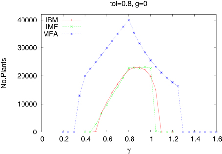
Figure 1. Number of plants as a function of water supply γ. One species. Homogeneous habitat. IBM, IMF, and MFA cases.

Clearly MFA gives much different results. It is possible, but at a quite large cost, to construct the MFA algorithm also for systems of many plants. Therefore, in the following we shall restrict the investigations to the IBM and IMF cases.

Let us now complicate the situation by considering a system of several, say 20, species, which differ only by their tolerances. We assume that the tolerances increase by 0.1 from the lowest value tl(1) equal 0.4. Introducing different types of plants means that there are cells containing seeds of different plants and we have to define the way one seed is chosen for germination. We follow here the lottery model of Chesson and Warner [43]. The probability of choosing a seed of a given species is equal to the fraction of such seeds in the cell. All other features of the model remain the same also for a system of many types of plants. We introduce at the beginning 500 plants of each species, located at random positions. In the neighborhood we do not distinguish types of plants, hence the factor nn_i means the number of nearest neighbors, irrespective of their type. Similarly in the IMF the density ϱ means the total density of all types of plants. Now the central question is not how many plants survived, but how many species are alive at the end of simulations when the rainfall γ is changing. The results are shown in Figure 2, for the two approaches—IBM and IMF. Averaging is over 500 independent runs, meaning that we start the simulations with the same number of plants, but placed in different positions, As we see, now the difference between the two approaches is quite large and simplifying the algorithm leads to reduction of the number of species alive. There is practically no difference between averaging over 100 and 500 runs.

FIGURE 2

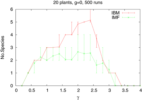
Figure 2. Number of species of 20 types as a function water supply γ for the IBM and IMF approach. Homogeneous habitat. The vertical lines indicates the statistical error bars.

Let us add another feature—the habitat will now be heterogeneous. We assume that the rainfall decreases in a given direction, say, along the X-axis, forming a gradient of steepness g. Such a situation is quite often encountered in nature where the plants are living on the slopes of a hill [44]. Heterogeneous environment is often regarded as one of the possible sources of maintaining biodiversity [45, 46]. When g = 0 we come back to the homogeneous habitat considered previously. Otherwise the amount of water for all cells having the coordinate x is equal

$\begin{array}{ll}\gamma (x)=\gamma \left(1-g\frac{x}{L}\right),& (46)\end{array}$

hence the rainfall decreases with x from its maximum value at x = 1 to its lowest at x = L. How the type of approach used influences the average number of species alive at the end of simulations, is shown in Figure 3 for the case of 20 species and medium value of the gradient (g = 0.5). The difference between the IBM and IMF methods is quite large and certainly now choosing IMF as a tool for studying systems of several plants, cannot be recommended. It should be also noted that while introduction of heterogeneous habitat leads to a large increase of the number of surviving species when the IBM method is used, it has rather weak effect for the IFM data.

FIGURE 3

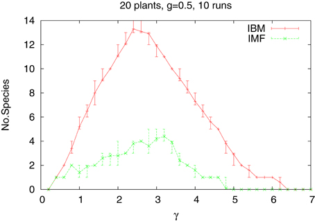
Figure 3. Same as above, but for heterogeneous habitat. Gradient of steepness 0.5. The vertical lines indicates the statistical error bars.

The differences are better seen in a more detailed study of a system of just five species with tolerances 0.6, 0.8, 1.0, 1.2, and 1.4. In Figure 4 we show the time dependence of the abundances of the five types of plants obtained from the IBM method and in the Figure 5 shown are the results from the IMF method. Habitat is heterogeneous with g = 0.5 and the rainfall is equal γ = 1.0 and 1.5. While coexistence of species is possible, also for extended time, within the IBM approach, simple IMF predicts that one species will soon dominate and eliminate all other, hence coexistence is impossible. How comes that in a more sophisticated method plants with different tolerances can exist in a heterogeneous habitat, is shown in Figures 6, 7. We see that different types of plants are able to colonize regions where the living conditions match their tolerance best. In these regions they can eliminate seeds of other types of plants, since they have the largest chance to germinate, then grow up and produce seeds, which, in the case of IBM, will be dispersed in the neighborhood. This means that in a given cell there will be more seeds of plants better fit to local conditions and therefore such seeds will be privileged by the lottery mechanism, forming a positive feedback. When the seeds are dispersed over the whole lattice some of them fall into rather hostile environment and even if one of them is chosen for germination it may not succeed in it. As the results many seeds are lost and eventually seeds from plants which have tolerances close to, but a bit lower than the actual value of the rainfall γ will be best off, as seen in Figure 7, since in many parts of the system they could find, if not ideal, at least satisfactory conditions for germination. Due to dispersal of seeds over the whole lattice, formation of local clusters of plants of the same type is impossible.

FIGURE 4

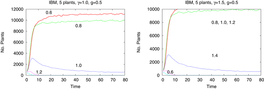
Figure 4. Number of plants of five types as a function of time in heterogeneous habitat. Left panel γ = 1.0, right panel γ = 1.5, IBM approach. Shown is a restricted time interval.

FIGURE 5

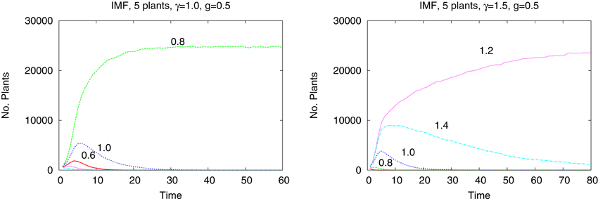
Figure 5. Same system as in the previous figure but in an IMF approach.

FIGURE 6

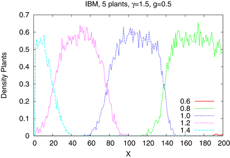
Figure 6. Density of plants of five types along the gradient. γ = 1.5. IBM approach.

FIGURE 7

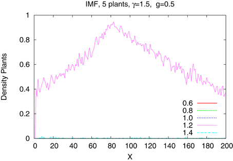
Figure 7. The same system as in the previous figure but for the IMF.

We have shown that in a very simple case of just one plant living in a homogeneous habitat using IMF or IBM does nor really matter. However, in more complex situations, like many species and/or heterogeneous environment, results coming from those two approaches could be vastly different. In particular, observed in nature long term coexistence of species cannot be obtained from the more simple IMF approach. The very crude MFA method always gives results differing from both IMF and IBM and therefore is not recommended in more detailed studies.

5. Conclusions

The problem of modeling complex systems is a difficult one and different levels of modeling are proposed in the literature. The simplest one uses mean-field like approximation while more sophisticated one are spatially extended models which are taking into account the local fluctuations of the relevant variables. The resolution of these more sophisticated models can be very complicated for several reasons among which the proliferation of the number of control parameters is an non-trivial one. An important point is that the predictions of the mean-field models may strongly differ from the ones given by more microscopic models. It would be important to have a criterion allowing us to decide if a simple mean-field like model is enough to describe the properties of a given system or not. As we have shown, except in some particular situations, there no such general criterion. In a large body of research papers this issue is simply ignored and conclusions are based on simple mean-field like models. This is why in this paper we wanted first to illustrate the importance of the fluctuations in a self-contained and pedagogical way, by revisiting two different classes of problems (equilibrium and non-equilibrium statistical mechanics) for which thorough studies on the role played by the fluctuations have been achieved. Second to apply these ideas to the study on an important question of biodiversity in which mean-field and more microscopic models lead to different predictions.

Author Contributions

MD wrote the Introduction, Equilibrium statistical physics, and Non-equilibrium statistical physics sections. AP wrote the section Plants dynamics and biodiversity. We both wrote the Conclusions. Research in the Plant dynamics part has been made in close cooperation.

Conflict of Interest Statement

The authors declare that the research was conducted in the absence of any commercial or financial relationships that could be construed as a potential conflict of interest.

References

1. Schilpp PA, Jehle H. Albert Einstein-philosopher-scientist. Am J Phys. (1951) 19:252–3.

Google Scholar

2. Van Vliet CM. Equilibrium and Non-equilibrium Statistical Mechanics. Singapore: World Scientific (2008).

Google Scholar

3. Landau L, Lifchitz E. Mécanique des Fluides, Mir Edn. Moscow (1971).

4. Chopard B, Droz M. Cellular Automata Modeling of Physical Systems, Vol. 6. Cambridge: Cambridge University Press (2005).

5. McCoy BM, Wu TT. The Two-Dimensional Ising Model. Boston, MA: Courier Corporation (2014).

Google Scholar

6. Droz M. Recent theoretical developments on the formation of Liesegang patterns. J Stat Phys. (2000) 101:509–19. doi: 10.1023/A:1026489416640

CrossRef Full Text | Google Scholar

7. Fisher RA. The wave of advance of advantageous genes. Ann Hum Genet. (1937) 7:355–69.

Google Scholar

8. Droz M. Modeling cooperative behavior in the social sciences. In: Eight Granada Lectures, AIP Proceedings 779. New York (2005).

9. Droz M, Pȩkalski A. Model of annual plants dynamics with facilitation and competition. J Theor Biol. (2013) 335:1–12. doi: 10.1016/j.jtbi.2013.06.010

PubMed Abstract | CrossRef Full Text | Google Scholar

10. Macal CM, North MJ. Tutorial on agent-based modeling and simulation. In: Proceedings of the 37th Conference on Winter Simulation. Argonne, IL: Winter Simulation Conference (2005). pp. 2–15.

11. Durrett R, Levin S. The importance of being discrete (and spatial). Theor Popul Biol. (1994) 46:363–94.

Google Scholar

12. Ising E. Beitrag zur theorie des ferromagnetismus. Z Phys A (1925) 31:253–8.

Google Scholar

13. Malarz K, Magdoń-Maksymowicz M, Maksymowicz A, Kawecka-Magiera B, Kułakowski K. New algorithm for the computation of the partition function for the Ising model on a square lattice. Int J Mod Phys C (2003) 14:689–94. doi: 10.1142/S012918310300484X

CrossRef Full Text | Google Scholar

14. Onsager L. Crystal statistics I. A two-dimensional model with an order-disorder transition. Phys Rev. (1944) 65:117.

Google Scholar

15. Binder K. Introduction: Theory and Technical Aspects of Monte Carlo Simulations. Heidelberg: Springer (1986).

Google Scholar

16. Curie P. Sur la possibilité d'existence du magnétisme libre. J Phys. (1894) 3:415.

17. Thompson CJ. Mathematical Statistical Mechanics. Princeton, NJ: Princeton University Press (2015).

Google Scholar

18. Kleinert H. Hubbard-Stratonovich transformation: Successes, failure, and cure. arXiv:1104.5161 (2011).

Google Scholar

19. Landau L, Lifchitz E. Physique Statistique. Mir Edn. Moscow (1967).

Google Scholar

20. Ben-Avraham D, Havlin S. Diffusion and Reactions in Fractals and Disordered Systems. Cambridge: Cambridge University Press (2000).

Google Scholar

21. Cantrell RS, Cosner C. Spatial Ecology via Reaction-Diffusion Equations. Chichester: John Wiley & Sons (2004).

Google Scholar

22. Zel'Dovich YB, Ovchinnikov A. The mass action law and the kinetics of chemical reactions with allowance for thermodynamic fluctuations of the density. Z Eksp Teor Fiz. (1978) 74:1588–98.

Google Scholar

23. Toussaint D, Wilczek F. Particle–antiparticle annihilation in diffusive motion. J Chem Phys. (1983) 78:2642–7.

Google Scholar

24. Kang K, Redner S. Scaling approach for the kinetics of recombination processes. Phys Rev Lett. (1984) 52:955.

Google Scholar

25. Chopard B, Droz M. Cellular automata model for the diffusion equation. J Stat Phys. (1991) 64:859–92.

Google Scholar

26. Grassberger P, Scheunert M. Fock-space methods for identical classical objects. Fortschr Phys. (1980) 28:547–78.

Google Scholar

27. Doi M. Stochastic theory of diffusion-controlled reaction. J Phys A Math Gen. (1976) 9:1479.

Google Scholar

28. Täuber UC, Howard M, Vollmayr-Lee BP. Applications of field-theoretic renormalization group methods to reaction–diffusion problems. J Phys A Math Gen. (2005) 38:R79. doi: 10.1088/0305-4470/38/17/R01

CrossRef Full Text | Google Scholar

29. Cardy JL, Täuber UC. Field theory of branching and annihilating random walks. J Stat Phys. (1998) 90:1–56.

Google Scholar

30. Cardy J. Renormalisation group approach to reaction-diffusion problems. arXiv cond-mat/9607163 (1996).

Google Scholar

31. Täuber UC. Renormalization group: applications in statistical physics. Nucl Phys B Proc Suppl. (2012) 228:7–34. doi: 10.1016/j.nuclphysbps.2012.06.002

CrossRef Full Text

32. Antal T, Droz M, Magnin J, Rácz Z. Formation of Liesegang patterns: a spinodal decomposition scenario. Phys Rev Lett. (1999) 83:2880.

Google Scholar

33. Gálfi L, Rácz Z. Properties of the reaction front in an A+B to C type reaction-diffusion process. Phys Rev A (1988) 38:3151.

PubMed Abstract | Google Scholar

34. Cornell S, Droz M, Chopard B. Some properties of the diffusion-limited reaction nA + mB to c with homogeneous and inhomogeneous initial conditions. Phys A Stat Mech Appl. (1992) 188:322–36.

Google Scholar

35. Cornell S, Droz M, Chopard B. Role of fluctuations for inhomogeneous reaction-diffusion phenomena. Phys Rev A (1991) 44:4826.

PubMed Abstract | Google Scholar

36. Ben-Naim E, Redner S. Inhomogeneous two-species annihilation in the steady state. J Phys A Math Gen. (1992) 25:L575.

Google Scholar

37. Cornell S, Droz M. Exotic reaction fronts in the steady state. Phys D Nonlinear Phenomena (1997) 103:348–56.

Google Scholar

38. Tardieu F. Virtual plants: modelling as a tool for the genomics of tolerance to water deficit. Trends Plant Sci. (2003) 8:9–14. doi: 10.1016/S1360-1385(02)00008-0

PubMed Abstract | CrossRef Full Text | Google Scholar

39. Ka̧cki Z, Pȩkalski A. The impact of competition and litter accumulation on germination success in a model of annual plants. Phys A (2011) 390:2520–30. doi: 10.1016/j.physa.2011.03.014

CrossRef Full Text | Google Scholar

40. Pȩkalski A, Szwabiński J. Dynamics of three types of annual plants competing for water and light. Phys A (2013) 392:710–21. doi: 10.1016/j.physa.2012.09.029

CrossRef Full Text

41. Schenk H. Root competition: beyond resource depletion. J Ecol. (2006) 94:725–39. doi: 10.1111/j.1365-2745.2006.01124.x

CrossRef Full Text | Google Scholar

42. Droz M, Pȩkalski A. Species richness in a model with resource gradient. Theor Ecol. (2016). doi: 10.1007/s12080-016-0298-8. [Epub ahead of print].

PubMed Abstract | CrossRef Full Text | Google Scholar

43. Chesson P, Warner R. Environmental variability promotes coexistence in lottery competitive systems. Am Nat. (1981) 117:923–43.

Google Scholar

44. Travis J, Brooker R, Clark E, Dytham C. The distribution of positive and negative species interactions across environmental gradients on a dual-lattice model. J Theor Biol. (2006) 241:896–902. doi: 10.1016/j.jtbi.2006.01.025

PubMed Abstract | CrossRef Full Text | Google Scholar

45. Tilman D. Competition and biodiversity in spatially structured habitats. Ecology (1994) 75:2–16.

Google Scholar

46. Holmes E, Wilson H. Running from trouble: long distance dispersal and the competitive coexistence of inferior species. Am Nat. (1998) 151:578–86.

PubMed Abstract | Google Scholar