Generalized Moment Analysis of Magnetic Field Correlations for Accumulations of Spherical and Cylindrical Magnetic Perturbers

1. Introduction

When exposed to an external magnetic field as in magnetic resonance imaging (MRI), spatial variations of magnetic susceptibility in heterogeneous systems such as biological tissue induce local inhomogeneities of the magnetic field that are usually visible for macroscopic structures. Susceptibility-weighted imaging and quantitative susceptibility mapping are MRI sequences that make use of this effect, e.g., to better visualize a cerebral thromboembolism or to quantify cerebral blood oxygen saturation [1, 2], and are therefore important in neuroradiological imaging. Susceptibility differences in biological tissue occur at the interfaces between different tissue structures and/or different types of tissue, thus generating local magnetic field gradients that lead to a dephasing of the magnetization. This effect can also be used to obtain quantifiable information on microscopic structures that are not resolvable in routine MRI due to technical limitations or optimization of measurement time. Such structures might be near-spherical as, for instance, iron accumulations in brain cells in neurodegenerative disease [3] or ultrasmall paramagnetic iron oxide particles that are ingested from macrophages in cell labeling techniques to allow assessment of the extent of cardiovascular disease [4], nerve injury [5], or to simply track immune cells [6]. Also, due to the BOLD effect [7], capillaries containing erythrocytes with deoxygenated hemoglobine possess an inherent paramagnetic susceptibility that is different to that of the surrounding tissue. For such magnetized spherical and cylindrical subvoxel structures, diffusion effects due to spin movements are not negligible. In fact, an increase of spin dephasing through diffusion effects may lead to a characteristic loss of inter-spin coherence: a spin that diffuses around these magnetic field perturbers experiences the local magnetic field inhomogeneities even though the applied external field is homogeneous. Diffusion effects for an ensemble of diffusing spins therefore lead to a more rapidly evolving phase decoherence than that expected from diffusion-free spin relaxation [8]. In addition, combined effects on dephasing of magnetic susceptibility and diffusion gradients are actively investigated, e.g., for diffusional kurtosis imaging [9]. In fact, some authors suggest that anomalous or non-Gaussian diffusion in biological tissue is due to dephasing effects that are promoted by both diffusion multi-compartmentalization and magnetic susceptibility [10, 11].

Previously, local susceptibility gradients and their effect on MR-signal behavior have been examined through spin-echo relaxation rates R₂ = 1/T₂ and gradient-echo relaxation rates $R_2^{*}=1/T_2^{*}$ [12–14], but, since magnetization does not necessarily decay monoexponentially ~ exp(−t/T₂) or $~\text{exp}(-t/T_2^{*})$ in time [15], a rightful interpretation of the signal evolution becomes cumbersome. Another approach is given by the frequency autocorrelation function K(t) that describes the transition probability of a spin from one local Larmor frequency state to the next in a specific time [16]. It is both sensitive to proton spin diffusion and the shape of the local magnetic field inhomogeneities. When spin dephasing around the local magnetic field inhomogeneity is Gaussian, a relation between magnetization time evolution and the frequency correlation function can be established [17] and it could be shown that information about correlation functions provide a more direct and measurable link to the local magnetic field inhomogeneity than relaxation rates [18]. Magnetic field correlation imaging techniques have already been utilized for MR measurements of iron accumulation in brain parenchyma [19] and for the MR-analysis of porous media [20]. In addition, since Carr-Purcell-Meiboom-Gill (CPMG) sequence relaxation rates are connected to the correlation function [16], a better knowledge of the correlation function may aid in determining microstrucutral parameters that quantify local capillary size, density, and oxygen extraction fraction in muscle tissue [21, 22].

Spin diffusion leads to a decrease of correlation over time that is mostly assumed to occur monoexponentially with a characteristic time constant or correlation time [23, 24], a simplification that is hardly valid for large parameter regimes. With this in mind, a detailed account of the intricate relation between magnetic field inhomogeneities and the frequency correlation function that characterizes the MRI relaxation process has been provided recently for restricted diffusion in Ziener et al. [25], and for unrestricted diffusion in Ayant et al. [26] and Sukstanskii et al. [27].

To account for the time dependence of microstructural quantities of the diffusion process, generalized moment expansion analysis can be employed to approximate their long time behavior. Generalized moment analysis is an extension of the first passage time approximation [28] and has been used to study, for instance, (non-)reactive processes that involve Brownian motion [29, 30], finite Ising systems [31], single-mode lasers [32], or to generally approximate autocorrelation functions [30]. In fact, the mean relaxation time approximation represents the lowest order approximation of the generalized moment expansion method and could be shown to better approximate the exact correlation function than the high-frequency i.e., short-time approximation used in conventional Padé approximations [30, 33].

In this work, the generalized moment analysis will be introduced and utilized to determine Padé approximants in the biexponential approximation for correlation functions of spherical and cylindrical magnetic objects. This analysis extends and furthers a preceding analysis that only considered the monoexponential decay forms for cylindrical magnetic perturbers [25].

2. Materials and Methods

The following analysis is based on the consideration of compact and impermeable objects G inside a voxel of size V_Voxel that are exposed to an external static magnetic field with strength B₀ (see Figure 1A). Assuming homogeneous diffusion properties in the dephasing volume V = V_Voxel − G, i.e., no barriers such as membranes or other materials, diffusing proton spins around object G are subject to stochastic field fluctuations induced by the distortion of the magnetic field in the vicinity of G.

FIGURE 1

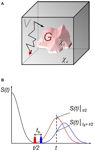
Figure 1. Proton spin trajectory around a magnetized object and measurement of the frequency correlation function through asymmetric spin echos. (A) Magnetized object G with susceptibility χ_i embedded in a surrounding medium V with susceptibility χ_e; both volumes constitute the voxel volume V_Voxel and the volume fraction is η = G/V_Voxel. The spin is subjected to stochastic field fluctuations in V induced by a distortion of the magnetic field from object G. (B) The corresponding frequency correlation function K(t) = 〈ω(t)ω(0)〉, where the bra-ket-formalism indicates averaging over all protons inside the voxel, determines the MR-signal S: through measurement of asymmetric spin echos, i.e., spin echos S(t)|_ts+t/2 that are shifted with time t_s away from the standard spin echo value of t/2 (see main text) we have $S(t){|}_{t_s+t/2}=S(t){|}_{t/2}\mathrm{\text{exp}}\left(-2{\mathit{\text{t}}}_{\mathit{\text{s}}}^2\mathit{\text{K}}\left(\frac{\mathit{\text{t}}}{2}\right)\right)$.

2.1. Frequency Autocorrelation Function

Generally, the distortion of the magnetic field is connected to the susceptibility difference Δχ = χ_i − χ_e between the magnetized object and its surrounding medium and leads to a variation in the local Larmor frequency

$\begin{array}{ll}\omega (r)=\delta \omega \frac{{\partial }^2}{\partial z^2}{\displaystyle {\int }_G\frac{{\text{d}}^3{r}^{\prime }}{|r-r^{\prime }|}},& (1)\end{array}$

with frequency shift δω = γB₀Δχ and gyromagnetic ratio γ = 2.675 × 10⁸s⁻¹T⁻¹ [34]. Let p(r, r₀, t) be the transition probability of a proton spin at point r and time t that started at position r₀ and time t = 0. Since, presumably, spin diffusion inside the dephasing volume encounters no barriers, transition probability p(r, r₀, t) is nothing less than the Green's function of the diffusion equation

$\begin{array}{ll}\frac{\partial }{\partial t}p(r,r_0,t)=D\Delta p(r,r_0,t),& (2)\end{array}$

where Δ denotes the Laplace operator and D is the diffusion coefficient. Thus,

$\begin{array}{ll}p(r,r_0,t)={\text{e}}^{tD\Delta }\delta (r-r_0),& (3)\end{array}$

and it is evident that p(r, r₀, t) only depends on the spatial difference r − r₀.

Then, to investigate stochastic field fluctuations around object G, a two-point correlation function K(t) can be introduced

$\begin{array}{ll}K(t)={\displaystyle {\int }_V{\text{d}}^3}r{\displaystyle {\int }_V{\text{d}}^3}{r}_0\omega (r)p(r,r_0,t)p(r_0)\omega (r_0)& (4)\end{array}$

$\begin{array}{ll}=\frac{1}{V}{\displaystyle {\int }_V{\text{d}}^3}r\omega (r){\text{e}}^{tD\Delta }\omega (r),& (5)\end{array}$

where we made use of Equation (3) in the last step. The probability density of the equilibrium p(r₀) = 1/V due to the assumption of homogeneous spin density. The frequency autocorrelation function K(t) is linked to the measured MR-signal S(t) and can be determined through measurement of asymmetric spin echos (see also Figure 1B and [18]). An asymmetric spin echo S(t)|_tp is a spin echo that is measured after a 180° refocusing pulse given at a time t_p ≠ t/2 where a refocusing pulse given at time t/2 corresponds to a symmetric spin echo S(t)|_t/2. When |t_p − t/2| = t_s, the following equality in our notation holds for low orders of t_s according to Jensen et al. [18]:

$\begin{array}{ll}S(t){|}_{t_s+t/2}=S(t){|}_{t/2}\exp \left(-2t_s^{2}K\left(\frac{t}{2}\right)\right).& (6)\end{array}$

Usually, Equation (6) is used in practice to be fitted to MRI data to obtain the correlation function.

2.2. Spherical and Cylindrical Magnetic Objects

In this work, two kinds of magnetic perturbers are considered: spheres and cylinders (see Figures 2A,B, respectively). For instance, an ensemble of microscopic spherical magnetic objects can represent the intracellular accumulation of iron particles in neurodegenerative disease [35] or the accumulation of ultrasmall paramagnetic iron oxide as a contrast agent to track macrophages in nerve injury or atherosclerotic disease [4, 5]. Collectives of cylindrical magnetic perturbers can be represented through a microvascular network in skeletal or cardiac muscle tissue [36, 37] where capillaries contain paramagnetic deoxygenated hemoglobine [7].

FIGURE 2

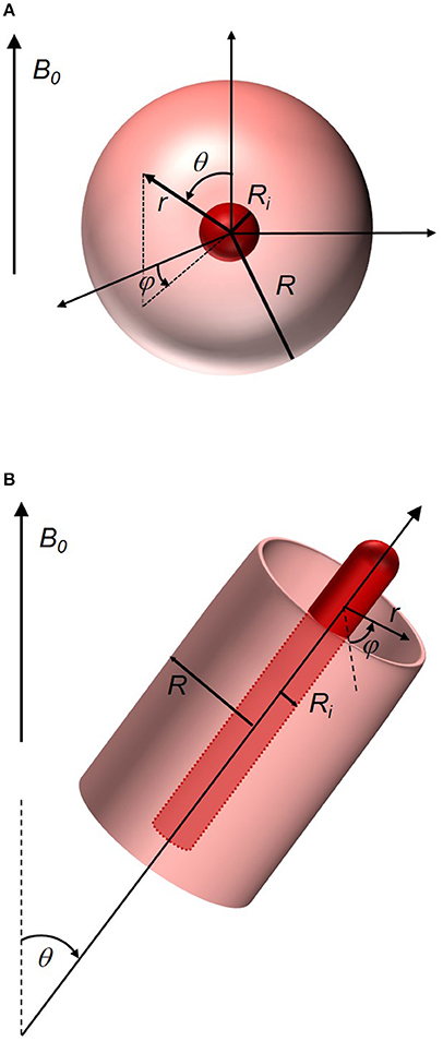
Figure 2. Spherical and cylindrical object in an external static magnetic field B₀. (A) Spherical magnetic object with radius R_i (red), that is surrounded by a dephasing volume sphere with radius R. The corresponding local Larmor frequency can be found in Equation (7). (B) Cylindrical object (red) with radius R_i of the cross section circle perpendicular to the cylinder axis. The cylinder is surrounded by a cylindrical dephasing volume with radius R. The angle θ between external magnetic field and cylinder axis is important in the determination of the local Lamor frequency in Equation (8).

The magnetic field around a spherical magnetic perturber is that of a magnetic dipole, i.e., with the external magnetic field B₀ being parallel to the z-axis of the coordinate system and utilization of spherical coordinates (r, θ, φ) (see also Figure 2A), the Larmor frequency reads

$\begin{array}{ll}\omega (r)=\delta \omega R_{\text{i}}^3\frac{3{\cos }^2(\theta )-1}{r^3}.& (7)\end{array}$

Here, $\delta \omega =\frac{1}{3}\gamma \Delta \chi B_0$ represents the frequency shift on the equatorial surface of the sphere with radius R_i. Its dephasing volume V ranges from the sphere surfaces to the surface of the mean relaxation volume. The latter depends on the form of the magnetized object and, therefore, the outer surface of V can be considered as a sphere with radius R. Consequently, the volume fraction of the magnetic material $\eta =R_{\mathrm{\text{i}}}^3/R^3$.

For a cylinder, the angle θ between its axis and the external magnetic field B₀ has to be acknowledged in the frequency shift to obtain the local frequency (see Figure 2B)

$\begin{array}{ll}\omega (r)=\delta \omega R_{\text{i}}^2\frac{\cos (2\phi )}{r^2},& (8)\end{array}$

where $\delta \omega =\frac{1}{2}\gamma \Delta \chi B_0{\text{sin}}^2(\theta )$ is the external frequency shift. In analogy to spheres, the local volume fraction $\eta =R_{\mathrm{\text{i}}}^2/R^2$ for a outer cylindrical surface of the dephasing volume with radius R. In both cases, the rationale of the approach has already been discussed in detail elsewhere [13, 38, 39].

For ensembles of several (microscopic) magnetic objects, it is helpful to avail oneself of the principle of supply areas as in the Krogh capillary model [40]. If the volume hosting the magnetic perturbers can be split into smaller volumes of similar geometry and if the local resonance frequency around the magnetic perturber is point symmetric, i.e., ω(r) = ω(−r) which is valid for both spheres and cylinders, it is possible to think of spin trajectories that leave their initial supply area or dephasing volume as being reflected at its boundary. Also, the same applies for spins whose trajectories hit the surface of the magnetic perturber that is assumed impermeable. Then, the Krogh model allows reducing the problem to one single object, i.e., diffusion is not considered in the whole tissue but, instead, for one single magnetic perturber only and reflective boundary conditions are assumed

$\begin{array}{ll}{\frac{\partial }{\partial r}p(r,r_0,t)|}_{r=R_{\text{i}}}=0={\frac{\partial }{\partial r}p(r,r_0,t)|}_{r=R}.& (9)\end{array}$

The case of unrestricted diffusion for a dephasing volume V extending from the surface of the magnetic perturber to infinity has already been analyzed in detail for spheres [26, 27, 41] and cylinders [27] and shall not be the subject of this investigation. It corresponds to very small volume fractions η ≈ G/V_Voxel where spin diffusion around the magnetic object does not reach the outer surface of V during the measurement. A detailed account in a similar notation can be found in Ziener et al. [25].

2.3. Eigenfunction Expansion

The diffusion equation (Equation 2) can be solved with the help of an eigenfunction expansion of the transition probability p(r, r₀, t):

$\begin{array}{l}p(r,r_0,t)={\displaystyle \sum _{{\kappa }_n\ge 0}^{\infty }{\text{e}}^{-{\kappa }_n^2\frac{Dt}{R_{\text{i}}^2}}}{\varphi }_n(r){\varphi }_n^{*}(r_0)\\ =\frac{1}{V}+{\displaystyle \sum _{{\kappa }_n>0}^{\infty }{\text{e}}^{-{\kappa }_n^2\frac{Dt}{R_{\text{i}}^2}}}{\varphi }_n(r){\varphi }_n^{*}(r_0).& (10)\end{array}$

The eigenfunctions ϕ_n are solutions of the eigenvalue equation

$\begin{array}{ll}\Delta {\varphi }_n(r)=-\frac{{\kappa }_n^2}{R_{\text{i}}^2}{\varphi }_n(r),& (11)\end{array}$

with eigenvalues κ_n, and, they fulfill the orthogonality condition

$\begin{array}{ll}{\displaystyle \int {\text{d}}^3}r{\varphi }_n(r){\varphi }_{n^{\prime }}^{*}(r)={\delta }_{n{n}^{\prime }},& (12)\end{array}$

where R_i is the radius of the inner sphere or cylinder, respectively. Thereby, the lowest eigenvalue κ₀ = 0 corresponds to the lowest eigenfunction ${\varphi }_0=1/\sqrt{V}$ [42]. The influence of diffusion is taken into account by the correlation time τ

$\begin{array}{ll}\tau =\frac{R_{\text{i}}^2}{D}.& (13)\end{array}$

By substituting the spectral expansion of the transition probability p(r, r₀, t) into the definition of the autocorrelation function (Equation 4), we obtain

$\begin{array}{ll}K(t)={\displaystyle \sum _{n=1}^{\infty }{F}_n^2}{\text{e}}^{-{\kappa }_n^2\frac{t}{\tau }}& (14)\end{array}$

with expansion coefficients

$\begin{array}{ll}{F}_n=\frac{1}{\sqrt{V}}{\displaystyle \int {\text{d}}^3}r\omega (r){\varphi }_n(r).& (15)\end{array}$

Since ${\varphi }_0(\text{r})=1/\sqrt{V}$, the expansion coefficient F₀ = 0 does not contribute to the correlation function.

Explicit expressions can be given for both spherical and cylindrical geometries; in the case of spheres, $F_n^2$ reads

$\begin{array}{ll}{F}_n^2=\frac{216}{5{\kappa }_n^2}\frac{\eta }{\eta -1}\frac{{\left[j_2^{\prime }\left(\frac{{\kappa }_n}{\sqrt[3]{\eta }}\right)-{\eta }^{\frac{4}{3}}{j}_2^{\prime }({\kappa }_n)\right]}^2}{[{\kappa }_n^2-6]{\left[j_2^{\prime }\left(\frac{{\kappa }_n}{\sqrt[3]{\eta }}\right)\right]}^2+{\eta }^{\frac{1}{3}}[6{\eta }^{\frac{2}{3}}-{\kappa }_n^2]{\left[j_2^{\prime }({\kappa }_n)\right]}^2},& (16)\end{array}$

with κ_n obeying the eigenvalue equation

$\begin{array}{ll}{j}_2^{\prime }({\kappa }_n)y_2^{\prime }\left(\frac{{\kappa }_n}{\sqrt[3]{\eta }}\right)=j_2^{\prime }\left(\frac{{\kappa }_n}{\sqrt[3]{\eta }}\right)y_2^{\prime }({\kappa }_n).& (17)\end{array}$

Functions $j_2^{\prime }$ and $y_2^{\prime }$ are the first derivatives of the spherical Bessel functions of the first and second kind, respectively [25]. An approximation for the first zero κ₁ is provided in Appendix A.

For cylinders, we have with cylindrical Bessel functions J₂ and Y₂ of the first and second kind, respectively,

$\begin{array}{ll}{F}_n^2=\frac{8}{{\kappa }_n^2}\frac{\eta }{\eta -1}\frac{{\left[J_2^{\prime }\left(\frac{{\kappa }_n}{\sqrt{\eta }}\right)-{\eta }^{\frac{3}{2}}{J}_2^{\prime }({\kappa }_n)\right]}^2}{\left[{\kappa }_n^2-4\right]{\left[J_2^{\prime }\left(\frac{{\kappa }_n}{\sqrt{\eta }}\right)\right]}^2+[4\eta -{\kappa }_n^2]{\left[J_2^{\prime }({\kappa }_n)\right]}^2},& (18)\end{array}$

and eigenvalues κ_n are the solution of

$\begin{array}{ll}{J}_2^{\prime }({\kappa }_n)Y_2^{\prime }\left(\frac{{\kappa }_n}{\sqrt{\eta }}\right)=J_2^{\prime }\left(\frac{{\kappa }_n}{\sqrt{\eta }}\right)Y_2^{\prime }({\kappa }_n).& (19)\end{array}$

The long time behavior of K(t) can be determined by considering the first eigenvalue κ₁ only:

$\begin{array}{ll}{K}_{\text{L}}(t)=F_1^2{\text{e}}^{-{\kappa }_1^2\frac{t}{\tau }}.& (20)\end{array}$

Evidently, K_L(t) converges asymptotically against zero for large t or K(∞) = 0. On the other hand, the value of the correlation function at t = 0 can be obtained by making use of Equation (3) with the initial condition p(r, r₀, 0) = δ(r − r₀):

$\begin{array}{ll}K(0)=\langle {\omega }^2(r)\rangle =\frac{1}{V}{\displaystyle {\int }_V{\text{d}}^3}r{\omega }^2(r)& (21)\end{array}$

$\begin{array}{ll}={\displaystyle \sum _{n=1}^{\infty }{F}_n^2}.& (22)\end{array}$

The last relation is useful for numerical computation and corresponds to Parseval's theorem in Fourier analysis.

2.4. Generalized Moment Analysis

The generalized moment expansion method or generalized moment approximation (GMA) has been used recently as an effective algorithm to approximate the time dependence of observables that are connected to reactive and non-reactive processes involving Brownian motion [29, 30, 43, 44]. It can be applied for monitoring diffusive redistributions and barrier crossing problems as well as to approximate autocorrelation functions [30]. In our case, the generalized moment analysis will be used to derive analytical expressions for the correlation function for biexponentially approximated decay forms that will prove to be more accurate than monoexponential approximations. The following subsections will introduce generalized moments and the Padé approximation and results from monoexponential approximations, as detailed in Ziener et al. [25], will be briefly recapitulated to give a buildup to biexponential approximations.

2.4.1. Generalized Moments

In using the Laplace transform $\widehat{K}(s)$ of the correlation function K(t) in Equation (5),

$\begin{array}{ll}\widehat{K}(s)=\frac{1}{V}{\displaystyle {\int }_V{\text{d}}^3}r\omega (r)\frac{1}{s-D\Delta }\omega (r),& (23)\end{array}$

it is convenient to expand $\widehat{K}(s)$ in a power series of 1/s and s for the short and long time behavior, respectively, as

$\begin{array}{ll}\underset{s\to 0}{\lim }\widehat{K}(s)={\displaystyle \sum _{n=0}^{\infty }{\mu }_{-(n+1)}}{[-s]}^n,& (24)\end{array}$

and

$\begin{array}{ll}\underset{s\to \infty }{\lim }\widehat{K}(s)=\frac{1}{s}{\displaystyle \sum _{n=0}^{\infty }{\mu }_n}{\left[-\frac{1}{s}\right]}^n.& (25)\end{array}$

The high-frequency moments μ_n hereby correspond to the short time behavior and the low-frequency moments μ_−(n+1) to the long time behavior. They are defined as

$\begin{array}{l}{\mu }_n=\frac{{[-1]}^n}{n!}\underset{s\to \infty }{\lim }\frac{{\text{d}}^n\left[s\widehat{K}(s)\right]}{\text{d}{\left[\frac{1}{s}\right]}^n}\\ =\underset{t\to 0}{\lim }\frac{{\text{d}}^{n}K(t)}{\text{d}{t}^n}& (26)\end{array}$

and

$\begin{array}{l}{\mu }_{-(n+1)}=\frac{{[-1]}^n}{n!}\underset{s\to 0}{\lim }\frac{{\text{d}}^n\widehat{K}(s)}{\text{d}{s}^n}\\ =\frac{1}{n!}{\displaystyle {\int }_0^{\infty }\text{d}}t{t}^{n}K(t),& (27)\end{array}$

respectively. Equation (5) allows combining the last two equalities into one expression for positive and negative n as

$\begin{array}{ll}{\mu }_n=\frac{1}{V}{\displaystyle {\int }_V{\text{d}}^3}r\omega (r){\left[-D\Delta \right]}^n\omega (r).& (28)\end{array}$

Therefore, the moments μ_n only depend on diffusion coefficient D and the form of the distortion of the magnetic field from magnetic perturber G. To avoid confusion, only one expression μ_n will be used below that refers to high-frequency moments for n ≥ 0 and to low-frequency moments for n < 0. For n = 0, the moment is identical to K(0) in Equation (21) and, therefore, corresponds to ${\mu }_0=\langle {\omega }^2(\text{r})\rangle$. The evaluation of Equation (28) for positive indices is straight-forward, whereas moments with a negative index n can be determined through quadratures, i.e.,

$\begin{array}{ll}{\mu }_{-n}=\frac{1}{V{D}^n}{\displaystyle {\int }_V{\text{d}}^3}r\omega (r)\underset{{\mu }_{-n}(r)}{\underbrace{{\left[-\Delta \right]}^{-n}\omega (r)}},& (29)\end{array}$

where the moment function μ_−n(r) for n ≥ 0 was introduced that satisfies

$\begin{array}{ll}{[-\Delta ]}^n{\mu }_{-n}(r)=\omega (r).& (30)\end{array}$

Thus, moments with negative index can be determined by solving the differential equation Equation (30) where μ_−n(r) obeys the same reflecting boundary conditions in Equation (9).

2.4.2. Padé Approximation

The frequency autocorrelation function K(t) can be approximated by the sum of N exponential decays as

$K(t)\approx k_{(N_h,N_l)}(t)={\displaystyle \sum _{n=1}^N{f}_{(N_h,N_l),n}}{\text{e}}^{-{\Gamma }_{(N_h,N_l),n}t},(31)$

with prefactors f_{(Nh, Nl), n} and decay constants Γ_{(Nh, Nl), n} that are related to the moments μ_n. The sum of the number of high frequency moments N_h and that of low frequency moments N_l equals the 2N parameters to be determined: N_h+N_l = 2N. Then, the Laplace transform of K(t) in Equation (23) can be written as a sum of Lorentzians as

$\widehat{K}(s)\approx {\widehat{k}}_{(N_h,N_l)}(s)={\displaystyle \sum _{n=1}^N\frac{f_{(N_h,N_l),n}}{s+{\Gamma }_{(N_h,N_l),n}}}.(32)$

Padé approximants $\widehat{k}(s)$ are required to accurately describe the high- and low-frequency behavior of $\widehat{K}(s)$ in Equations (24) and (25) to a desired degree and to correctly reproduce the N_h high- and N_l low-frequency moments. The resulting description of the (N_h, N_l)-generalized-moment approximation, denoted as (N_h, N_l)-GMA, is a two-sided Padé approximation around s = 0 and s = ∞ [45]. When introducing the Padé approximation of the frequency autocorrelation function according to Equation (31) into the definition of the high and low frequency moments according to Equations (26) and (27), the parameters f_{(Nh, Nl), n} and Γ_{(Nh, Nl), n} can be obtained through

$\begin{array}{l}{\displaystyle \sum _{n=1}^N{f}_{(N_h,N_l),n}}{\Gamma }_{(N_h,N_l),n}^m={\mu }_m,\text{with }\\ m=-N_l,\dots ,N_h-1.& (33)\end{array}$

The generalized moments μ_n are closely related to the shape of the local field inhomogeneity as shown above and parameters f_{(Nh, Nl), n} and Γ_{(Nh, Nl), n} can be determined by the multi-exponential approximation of the correlation function in Equation (31). Therefore, an approximation of the correlation function is given through the solution of Equation (33), provided that the generalized moments μ_n are known.

3. Results

In the following, the correlation function within the GMA is derived for the biexponential approximation (N = 2) in the spherical and cylindrical model geometry, since it is then possible to provide an algebraic solution of Equation (33). However, the numerical solution for N > 2 is still possible by means of an equivalent eigenvalue problem [44, 46]. The case N = 1 was treated in Ziener et al. [25] and is presented in Appendix B for the sake of completeness.

For N = 2, the approximation of the correlation function can be extended to the sum of two exponential decays and Equation (33) leads to the sum

$\begin{array}{l}{f}_{(N_h,N_l),1}{\Gamma }_{(N_h,N_l),1}^m+f_{(N_h,N_l),2}{\Gamma }_{(N_h,N_l),2}^m={\mu }_m,\text{with}\\ m=-N_l,\dots ,-N_l+4.& (34)\end{array}$

In this work, two cases are being considered. The first case is the (2, 2)-GMA reproducing the moments μ₋₂, μ₋₁, μ₀, and μ₁ of the exact correlation function. To find the best approximation for the long time behavior, we choose the (1, 3)-GMA that reproduces the moments μ₋₃, μ₋₂, μ₋₁, and μ₀, i.e., more low-frequency moments are being taken into account. Introducing the following abbreviations

$\begin{array}{l}A={\mu }_{-1}^2-{\mu }_0{\mu }_{-2},\\ B={\mu }_0{\mu }_{-1}-{\mu }_1{\mu }_{-2},\\ C={\mu }_0^2-{\mu }_1{\mu }_{-1},\\ D={\mu }_{-1}{\mu }_{-2}-{\mu }_0{\mu }_{-3},\\ E={\mu }_{-2}^2-{\mu }_{-1}{\mu }_{-3},& (35)\end{array}$

we find for the (2, 2)-GMA the parameters

$\begin{array}{l}{\Gamma }_{(2,2),1}=\frac{B+\sqrt{B^2-4AC}}{2A},\\ {\Gamma }_{(2,2),2}=\frac{B-\sqrt{B^2-4AC}}{2A},\\ f_{(2,2),1}=+\frac{{\Gamma }_{(2,2),2}{\mu }_0-{\mu }_1}{{\Gamma }_{(2,2),2}-{\Gamma }_{(2,2),1}},\\ f_{(2,2),2}=-\frac{{\Gamma }_{(2,2),1}{\mu }_0-{\mu }_1}{{\Gamma }_{(2,2),2}-{\Gamma }_{(2,2),1}}.& (36)\end{array}$

Consequently, the correlation function for short times can be approximated as

$K_{(2,2)}(t)=f_{(2,2),1}{\text{e}}^{-{\Gamma }_{(2,2),1}t}+f_{(2,2),2}{\text{e}}^{-{\Gamma }_{(2,2),2}t}.(37)$

Similar results have been obtained by Bauer et al. [31] and Barsky et al. [47]: Equations (3.19–3.22) in Bauer et al. [31] as well as Equations (B15–B19) in Barsky et al. [47] are in agreement with the coefficients in Equation (35).

The second case of the (1, 3)-GMA yields parameters

$\begin{array}{l}{\Gamma }_{(1,3),1}=\frac{2A}{D-\sqrt{D^2-4AE}},\\ {\Gamma }_{(1,3),2}=\frac{2A}{D+\sqrt{D^2-4AE}},\\ f_{(1,3),1}=+\frac{{\mu }_{-1}-{\mu }_0{\Gamma }_{(1,3),2}^{-1}}{{\Gamma }_{(1,3),1}^{-1}-{\Gamma }_{(1,3),2}^{-1}},\\ f_{(1,3),2}=-\frac{{\mu }_{-1}-{\mu }_0{\Gamma }_{(1,3),1}^{-1}}{{\Gamma }_{(1,3),1}^{-1}-{\Gamma }_{(1,3),2}^{-1}},& (38)\end{array}$

and, consequently, the correlation function for long times reads

$K_{(1,3)}(t)=f_{(1,3),1}{\text{e}}^{-{\Gamma }_{(1,3),1}t}+f_{(1,3),2}{\text{e}}^{-{\Gamma }_{(1,3),2}t}.(39)$

Similar expression could be derived by Bauer and Schulten [38].

Introducing the above results for the biexponential approximation in the (2, 2)- and (1, 3)-GMA into Equation (31) determines the corresponding correlation function at t = 0 :

$K_{(2,2)}(t=0)=K_{(1,3)}(t=0)={\mu }_0=\langle {\omega }^2(r)\rangle ,(40)$

which is in agreement with the generally valid Equation (21). In the following sections, the time evolution of the two biexponential approximations in the GMA for the correlation function are exemplified for both spherical and cylindrical objects, respectively (see below).

3.1. Spheres

In order to solve differential equation (Equation 30) for spherical magnetic objects, it is helpful to start with the ansatz

${\mu }_{-n}(r)=\delta \omega R_{\text{i}}^3{\mu }_{-n}(r)[3{\cos }^2(\theta )-1](41)$

that separates the angle dependent part of the local Larmor frequency given in Equation (7). Also, the radial part of the Laplace operator can be written as

${\Delta }_{d,r}=\frac{1}{r^{d-1}}\frac{\text{d}}{\text{d}r}{r}^{d-1}\frac{\text{d}}{\text{d}r}(42)$

with d = 3 for spheres and d = 2 for infinitely long cylinders. This leads to an iterative set of equations for the functions μ_−n(r) of the form

$\left[{\Delta }_{3,r}-\frac{6}{r^2}\right]{\mu }_{-n}(r)=-{\mu }_{-(n-1)}(r),(43)$

or, equivalently,

${\mu }_{-n}(r)={\left[\frac{6}{r^2}-{\Delta }_{3,r}\right]}^{-n}\frac{1}{r^3}.(44)$

The differential equation (Equation 43) can be transformed to an Euler type differential equation. Using the general expression (Equation 41) for the solution of the differential equation (Equation 30), where the local Larmor frequency corresponds to Equation (7), the low-frequency moments given in Equation (28) can be found as

${\mu }_{-n}=\frac{12}{5}\frac{\delta {\omega }^2}{D^n}\frac{\eta }{1-\eta }{R}_{\text{i}}^3{\displaystyle \underset{R_{\text{i}}}{\overset{R}{\int }}\text{d}}r\frac{{\mu }_{-n}(r)}{r}.(45)$

The evaluation of the integral yields the general form

$\begin{array}{ll}{\mu }_n=\frac{\delta {\omega }^2}{{\tau }^n}{l}_n(\eta ).& (46)\end{array}$

For spherical geometries, the functions μ_n(r) can be found as the solution of Equation (43). The recursion starts with μ₀(r) which results from Equation (44). The functions are given by

$\begin{array}{l}{\mu }_0(r)=\frac{1}{r^3},\hfill \\ {\mu }_{-1}(r)=\frac{1}{6r}\left[1+\frac{c_1}{3}{\left[\frac{r}{R_i}\right]}^{-2}+\frac{c_2}{2}{\left[\frac{r}{R_i}\right]}^3\right],\hfill \\ {\mu }_{-2}(r)=\frac{r}{6}\left[\frac{1}{4}+\frac{c_1}{18}{\left[\frac{r}{R_i}\right]}^{-2}\text{}\text{}\text{}-\frac{c_2}{28}{\left[\frac{r}{R_i}\right]}^3\text{}\text{}\text{}+\text{}\frac{c_3}{3}{\left[\frac{r}{R_i}\right]}^{-4}\text{}\text{}\text{}+\frac{c_4}{2}\frac{r}{R_i}\right],\hfill \\ \begin{array}{l}{\mu }_{-3}(r)=\frac{r^3}{6}[-\frac{1}{24}+\frac{c_1}{72}{\left[\frac{r}{R_i}\right]}^{-2}\text{}\text{}\text{}+\frac{c_2}{1008}{\left[\frac{r}{R_i}\right]}^3\text{}\text{}\text{}+\frac{c_3}{18}{\left[\frac{r}{R_i}\right]}^{-4}\\ -\frac{c_4}{28}\frac{r}{R_i}+\frac{c_5}{3}{\left[\frac{r}{R_i}\right]}^{-6}+\frac{c_6}{2}{\left[\frac{r}{R_i}\right]}^{-1}].(47)\end{array}\hfill \end{array}$

We have used the abbreviation

$\begin{array}{ll}{d}_i={\displaystyle \sum _{j=0}^i}{\eta }^{\frac{j}{3}}& (48)\end{array}$

and the constants c₁, …, c₆ that are given by

$\begin{array}{l}{c}_1=-\frac{d_2}{d_4},\\ c_2=1+c_1,\\ c_3=\frac{25}{126}{\eta }^{\frac{1}{3}}\frac{d_1^2}{d_4^2}+\frac{11}{36d_4},\\ c_4=c_3-\frac{3}{28}-\frac{25}{126}\frac{d_2}{d_4},\\ c_5=\frac{61}{588}\left[{\eta }^{-\frac{1}{3}}-\frac{d_3}{d_4}\right]-\frac{625}{15876}\frac{\eta -2d_1}{d_4^3}\\ -\frac{5}{31752}\frac{331d_2+250d_1+232}{d_4^2},\\ c_6=c_5+\frac{61}{588}+\frac{625}{15876}{\eta }^{\frac{1}{3}}\frac{d_1^2}{d_4^2}+\frac{5}{31752}\frac{385-54d_2}{d_4},& (49)\end{array}$

where $\eta =R_{\mathrm{\text{i}}}^3/R^3$. The functions l_n(η) are necessary to determine the moments μ_n in Equation (46) for negative indices from Equation (45). They are given by

$\begin{array}{cc}\begin{array}{l}{l}_1(\eta )=\frac{126}{25}\frac{\eta }{1-\eta },\hfill \\ l_0(\eta )=\frac{4}{5}\eta ,\hfill \\ l_{-1}(\eta )=\frac{\eta }{90}\frac{32[1+{\eta }^{4/3}]+37[{\eta }^{1/3}+\eta ]+42{\eta }^{2/3}}{[{\eta }^{2/3}+{\eta }^{1/3}+1][{\eta }^{4/3}+\eta +{\eta }^{2/3}+{\eta }^{1/3}+1]},\hfill \\ \hfill & \hfill \\ l_{-2}(\eta )=\frac{{\eta }^{2/3}[972[1+{\eta }^{8/3}]+1684[{\eta }^{1/3}+{\eta }^{7/3}]+2271[{\eta }^{2/3}+{\eta }^2]+2733[\eta +{\eta }^{5/3}]+3580{\eta }^{4/3}]}{11340[{\eta }^{2/3}+{\eta }^{1/3}+1]{[{\eta }^{4/3}+\eta +{\eta }^{2/3}+{\eta }^{1/3}+1]}^2},\hfill \\ l_{-3}(\eta )=\frac{1}{1143072[{\eta }^{2/3}+{\eta }^{1/3}+1]{[{\eta }^{4/3}+\eta +{\eta }^{2/3}+{\eta }^{1/3}+1]}^3}\hfill \\ \times [6021[1+{\eta }^{14/3}]+24084[{\eta }^{1/3}+{\eta }^{13/3}]+47034[{\eta }^{2/3}+{\eta }^4]+80260[\eta +{\eta }^{11/3}]\hfill \\ +125533[{\eta }^{4/3}+{\eta }^{10/3}]+180466[{\eta }^{5/3}+{\eta }^3]+215176[{\eta }^2+{\eta }^{8/3}]+230452{\eta }^{7/3}].\hfill \end{array}& \left(50\right)\end{array}$

It is convenient to define a ratio τ_n of successive moments as

$\begin{array}{ll}{\tau }_n=\left|\frac{{\mu }_n}{{\mu }_{n+1}}\right|.& (51)\end{array}$

As in Ziener et al. [25], we make use of Koenig's theorem [48, 49] on the zeros of Padé approximants [48, 49]: the theorem states that the series 1/τ_n converges to the lowest eigenvalue of Equation (11) and [39], since then

$\begin{array}{ll}{\kappa }_1^2=\tau {\displaystyle \underset{n\to \infty }{\text{lim}}}\frac{{\mu }_{-n}}{{\mu }_{-(n+1)}},& (52)\end{array}$

where τ is the correlation time from Equation (13). The lowest eigenvalue κ₁ is the solution to the geometry-dependent eigenvalue equation, i.e., Equation (17) for spheres and Equation (19) for cylinders. In Figure 3, a sequence of successive moment ratios τ_n ranging from n = −3, …, 0 is compared with the exact numerical solution for κ₁ for spherical magnetic objects and Koenig's theorem is nicely exemplified for η → 1. The asymptotic value of the first eigenvalue for large volume fractions could be determined as ${\text{lim}}_{\eta \to 1}{\kappa }_1^2(\eta )=6$ for spheres and ${\text{lim}}_{\eta \to 1}{\kappa }_1^2(\eta )=4$ for cylinders (from Equations [A14] and [A5] in Ziener et al. [25], respectively), simply stating that, in this limit, the correlation function decays monoexponentially with time constant ${\kappa }_1^2$. An approximation for κ₁ is provided in Appendix A. Figure 3 also validifies the concept of generalized moments to define a search interval for numerical computation of the exact solution from Equations (17) and (19). However, the successive moments curves diverge from the exact solution for small volume fractions.

FIGURE 3

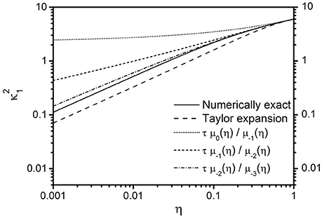
Figure 3. Dependence of successive moment ratios on the volume fraction for spherical magnetic objects. The ratio of successive moments τμ_−n(η)/μ_−(n+1)(η) = l_−n(η)/l_−(n+1)(η) in dependence on volume fraction η is obtained from Equation (46) [functions l_−n(η) are given in Equation (50)]. The numerically exact eigenvalue (solid line) can be obtained by solving Equation (17). An approximate solution for ${\kappa }_1^2$ (dashed line), based on a Taylor expansion, is given in Equation (A3) in Appendix A. For η → 1, all graphs asymptotically converge to the value ${\kappa }_1^2=6$. A visualization of the dependence of the ratio of successive moments on the volume fraction for cylinders with a slightly different notation is given in Figure 9 in Ziener et al. [25]. It can be obtained from Equation (46) with quantities δω, τ, and l_n(η) determined from the cylindrical geometry.

Different cases of the monoexponential functions K_i(t) (see Appendix B and Equation B3) are being shown in Figure 4A to demonstrate the dependence of the monoexponential approximation on the chosen moments μ_n. Evidently, the initial value of K_i(t), i ≥ 1, decreases with increasing i while the exponential cutoff begins at longer times for increasing i. Also, the approximants K_i(t) converge to the long time behavior given in Equation (20), as expected from Koenig's theorem. To evaluate the accuracy of the biexponential approximation, a double logarithmic plot has been chosen in Figure 4B. The (2, 2)-GMA with the two lowest high and low frequency moments approximates the short as well as the long time limit sufficiently well. In contrast, the (1, 3)-GMA with the three lowest low and the first high frequency moment approximates the long time limit significantly better than the short time limit. An application to biological tissue is provided in Figure 4C where mono- and bi-exponential approximations in the GMA of the correlation function are visualized for values that are typical for susceptibility gradients based on nonheme iron-storage in brain tissue (through iron-rich oligodendrocytes in the Globus pallidus that approximately have radii R_i of 3–4 μm, a frequency shift of δω = 184 s⁻¹, a tissue density of η = 0.04 and D = 0.76·10⁻⁹m²s⁻¹, leading to τ = 16.12 ms; see [50, 51] for more details). It can be seen that the biexponential approximations K_{(1, 3)}(t) and K_{(2, 2)}(t) are in excellent agreement with the actual correlation function K(t), while the monoexponential functions K_i(t) only approximate K(t) sufficiently for t ≳ 30 ms. However, changes in the size R_i of the spherical perturbers affect the correlation time τ as well according to Equation (13). The correlation function in dependence on correlation time τ is therefore shown in Figure 4D at the characteristic time t = 10 ms for the same set of mono- and bi-exponential approximations as in Figure 4C. In this case, the biexponential approximations show an equally well agreement with the numerically obtained correlation function K(τ) for all correlation times, whereas the monoexponential approximations exhibit significant deviations from K(τ) for correlation times that range from 40 ms to 5 s. For very short and very long correlation times, however, the monoexponential approximations K₀(τ) and K₁(τ) coincide with K(τ). Mono- and bi-exponential approximations as compared to K(t) for nanoparticle experiments based on parameters in Muller et al. [52], and for lung tissue based on parameters given in Stone et al. [53] and Baete et al. [54], are shown in Appendix C.

FIGURE 4

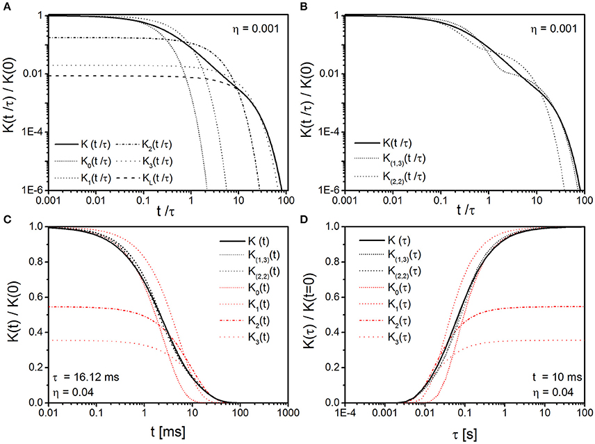
Figure 4. Mono- and bi-exponential approximation in the GMA of spherical objects. (A) Monoexponential approximations K_i(t) of the correlation function K(t) (solid line) as obtained from Equation (B3) with moments given in Schulten et al. [46]. The long time approximation K_L(t) (dashed line) is given by Equation (20) where the first eigenvalue κ₁ is determined by Equation (17) (η = 0.001 in A,B). (B) Biexponential approximations for long times K_{(1, 3)}(t) [dashed line obtained from Equation (39)] and for short times K_{(2, 2)}(t) [dotted line obtained from Equation (37)] of the correlation function K(t) [solid line obtained from Equation (14)]. Evidently, for spherical objects, the biexponential approximations are more accurate than monoexponential approximations and show a better agreement for large and short times with the actual correlation function K(t). (C) Mono- and bi-exponential approximations of K(t) for typical parameters of iron-storage in oligodendrocytes of the Globus pallidus, see main text for details. K_{(1, 3)}(t) and K_{(2, 2)}(t) both show an excellent agreement with K(t) whereas the monoexponential approximations exhibit significant deviations from K(t) for t ≲ 30 ms. (D) Correlation function approximations in dependence on correlation time τ at time-point t = 10 ms for otherwise equal parameters as in (C). The agreement of biexponential approximations with K(t) is excellent for all correlation times, whereas the monoexponential approximations mainly agree with K(t) for very short or very long correlation times.

3.2. Cylinders

In analogy to spherical magnetic objects, the correlation functions for spins that diffuse between two concentric cylinders can be obtained within the GMA by employing a similar ansatz as the one for a spherical geometry and by using Equation (42) for d = 2 as shown in Ziener et al. [25]. Then, generalized moments are determined by the differential equation

$\begin{array}{ll}{\mu }_{-n}(r)={\left[\frac{4}{r^2}-{\Delta }_{2,r}\right]}^{-n}\frac{1}{r^2}.& (53)\end{array}$

Again, for n = 0, 1, 2, 3, the functions μ_−n(r) for cylindrical geometries that obey Equation (53) can be determined as

$\begin{array}{cc}\begin{array}{l}{\mu }_0(r)=\frac{1}{r^2},\\ {\mu }_{-1}(r)=\frac{1}{4},\\ {\mu }_{-2}(r)=-\frac{r^2}{16}\left[\text{ln}\left(\frac{r}{R_{\text{i}}}\right)+c_1{\left[\frac{r}{R_{\text{i}}}\right]}^{-4}+c_2\right],\\ {\mu }_{-3}(r)=\frac{r^4}{192}[\text{ln}\left(\frac{r}{R_{\text{i}}}\right)+c_3{\left[\frac{r}{R_{\text{i}}}\right]}^{-4}+c_4+c_5{\left[\frac{r}{R_{\text{i}}}\right]}^{-6}\\ +c_6{\left[\frac{r}{R_{\text{i}}}\right]}^{-2}],\end{array}& \left(54\right)\end{array}$

and the constants c₁, …, c₆ are given by

$\begin{array}{rcl}{c}_1& =& \frac{1}{2}\frac{\mathrm{\text{ln}}(\eta )}{1-{\eta }^2},\\ c_2& =& c_1-\frac{1}{2},\\ c_3& =& -3c_1,\\ c_4& =& \frac{6}{7}\left[c_1-1\right],\\ c_5& =& \frac{1}{1+\eta }\left[2c_1+\frac{11}{6\eta }\right],\\ c_6& =& \frac{\eta }{1+\eta }\left[\frac{11}{6}\left[1+\frac{1}{\eta }+\frac{1}{{\eta }^2}\right]-2c_1\right].& (55)\end{array}$

The functions l_n(η) are obtained in analogy to the spherical case and are given as

$\begin{array}{lll}{l}_1(\eta )& =& 2\eta \left[1+\eta \right],\\ l_0(\eta )& =& \frac{\eta }{2},\\ l_{-1}(\eta )& =& \frac{1}{8}\frac{\eta \mathrm{\text{ln}}(\eta )}{\eta -1},\\ l_{-2}(\eta )& =& \frac{1}{32},\\ l_{-3}(\eta )& =& \frac{1}{256}\frac{\eta }{1-\eta }\left[\frac{3}{4}\frac{1-{\eta }^2}{{\eta }^2}+\frac{{\left[\mathrm{\text{ln}}(\eta )\right]}^2}{1-{\eta }^2}\right].& (56)\end{array}$

As in the case for spheres, the low-frequency moments μ_−n for cylinders from Equation (28) can be expressed as

$\begin{array}{ll}{\mu }_{-n}=\frac{\delta {\omega }^2}{D^n}\frac{\eta }{1-\eta }{R}_{\mathrm{\text{i}}}^2{\displaystyle \underset{R_{\mathrm{\text{i}}}}{\overset{R}{\int }}}\mathrm{\text{d}}r\frac{{\mu }_{-n}(r)}{r},& (57)\end{array}$

that correspond to Equation (77) in Ziener et al. [25]. Evaluation of the integral leads to Equation (46), but with the respective values of δω, τ, and l_n(η) for cylinders (see Equation 56).

In analogy to Figure 4A, the time evolution of the functions K_i(t) and their proximity to the long time approximation K_L(t) from Equation (20) is shown in Figure 5A. As in the spherical case, the initial value of K_i(t), i ≥ 1, decreases with increasing i and successive moments converge to the long time approximation K_L(t) for d = 2.

FIGURE 5

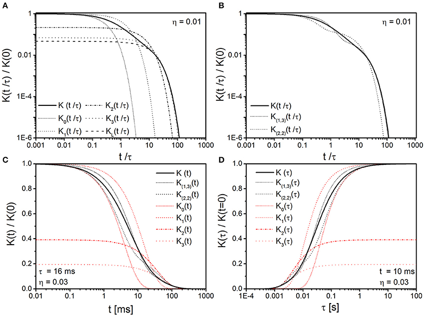
Figure 5. Mono- and bi-exponential approximation in the GMA of cylindrical objects. (A) Monoexponential approximations K_i(t) of the correlation function K(t) (solid line) as obtained from Equation (B3) with moments given in Schulten et al. [46]. The long time approximation K_L(t) (dashed line) is given by Equation (20) where the first eigenvalue κ₁ is determined by Equation (19) (η = 0.01 in A,B). (B) Biexponential approximations for long times K_{(1, 3)}(t) [dashed line obtained from Equation (39)] and for short times K_{(2, 2)}(t) [dotted line obtained from Equation (37)] of the correlation function K(t) [solid line obtained from Equation (14)]. As in the case for spherical objects, the biexponential approximations of the correlation function for cylindrical objects show a better asymptotic agreement with the actual correlation function K(t) than monoexponential approximations. (C) Mono- and bi-exponential approximations of the correlation function for typical parameters of capillaries in brain tissue, see main text for details. The deviations of the biexponential approximations from K(t) are visibly smaller than that of the monoexponential approximations. (D) Mono- and bi-exponential approximations of the correlation function in dependence on correlation time τ at time-point t = 10 ms, for otherwise equal parameters as in (C). The approximations K₀(τ), K₁(τ), K_{(1, 3)}(τ), and K_{(2, 2)}(τ) coincide with K(t) for very short and very long correlation times, whereas correlation function K(τ) for intermediate correlation times between 1 ms and 1 s is best approximated by the biexponential approximations.

In comparison, the biexponential approximation is shown in Figure 5B: for the (2, 2)- and the (1, 3)-GMA it can be seen that the first approximation describes short and long time limit sufficiently well whereas the second approximation is more accurate in the long time limit. An application to biological tissue is provided in Figure 5C where mono- and bi-exponential approximations in the GMA of the correlation function are visualized for values that are typical for susceptibility gradients between capillaries, that contain deoxygenated hemoglobine, and the surrounding tissue [with approximate values R_i = 4 μm [55], δω = 200 s⁻¹ at 3 Tesla [12, 56], a tissue density of η = 0.03 [55], and D = 1·10⁻⁹m²s⁻¹ [57], leading to τ = 16 ms]. It can be seen that the biexponential approximations K_{(1, 3)}(t) and K_{(2, 2)}(t) are in excellent agreement with the actual correlation function K(t) for t ≳ 20 ms, while only the monoexponential functions K₂(t) and K₃(t) sufficiently approximate K(t) for t≳ 80 ms. Still, the deviation of the biexponential approximations to K(t) for t < 30 ms are visibly smaller than for the monoexponential approximations. However, changes in the size R_i of the cylindrical perturbers affect the correlation time τ as well according to Equation (13). The correlation function in dependence on correlation time τ is therefore shown in Figure 5D at the characteristic time t = 10 ms for the same set of mono- and bi-exponential approximations as in Figure 5C. In this case, the biexponential approximations show an equally well agreement with the numerically obtained correlation function K(τ), especially for correlation times τ ≲ 50 ms, whereas the monoexponential approximations exhibit significant deviations from K(τ) for correlation times that range from 1 ms to 5 s. For very short and very long correlation times, however, the monoexponential approximations K₀(τ) and K₁(τ) coincide with K(τ), as in the case of spherical perturbers.

4. Discussion and Conclusions

The incentive of this work was to gain a better understanding of the dynamic frequency correlation function of spins that diffuse around microscopic magnetized objects. The analysis is based on an eigenfunction expansion of the correlation function where eigenfunctions and eigenvalues can be determined in the case of restricted diffusion through reflective boundary conditions. A two-sided Padé approximation is then utilized to derive analytical expressions in the short and long time limit. The different regimes of the functional form of the correlation function as well as the case of unrestricted diffusion have been studied in a preceding analysis that considered a monoexponentially decaying correlation function in the generalized moment approximation (GMA) for cylindrical magnetic objects [25]. The here-presented analysis extends and furthers this prior work to include biexponentially decaying correlation functions in the GMA for both high and low frequency moments and both spherical and cylindrical magnetic field perturbers, respectively. Expressions for four generalized moments in both model geometries are provided. They allow to determine the corresponding parameters of Padé aproximants for small and large times. Also, successive generalized moment ratios are shown to asymptotically converge to the exact first eigenvalue of the underlying spherical and cylindrical model geometry eigenvalue (Equations 17, 19), respectively, in agreement with Koenig's theorem.

The model with its boundary conditions is based on a presumed regular arrangement of accumulations of similarly shaped objects that can then be considered in analogy to Krogh's model for supply volumes around capillaries [40]. Thus, large volume fractions or the long time limit of spin diffusion processes can be examined for a point-symmetric local Larmor frequency where diffusion trajectories into a neighboring supply volume are thought of as being reflected at the boundary to said volume. More detailed accounts about the case of unrestricted diffusion can be found in Yablonskiy et al. [12], Ziener et al. [25], Ayant et al. [26], and Ziener et al. [58]. With Figures 4, 5 it can be seen that biexponential approximations in the GMA for K_{(1, 3)}(t) and K_{(2, 2)}(t) and for both spherical and cylindrical model geometries are in much better agreement with the actual correlation function K(t) than monoexponential approximations such as the frequently used “mean correlation time approximation” [38]. Comparisons of the approximations are also provided for iron-accumulations in brain tissue and for cerebral cortex capillaries in Figures 4C,D, 5C,D, respectively. Both cases demonstrate that there are pronounced differences between mono- and bi-exponential approximations for t ~ 1 − 100 ms, with the biexponential approximations providing the better approximations to the correlation function for all time-points. These results are therefore relevant for diffusion MRI experiments applied to these tissue types since the typical diffusion time during which the diffusion process can be detected in such an experiment ranges between 1 ms and 1 s. However, for very short correlation times (e.g., iron-oxide nanoparticle suspensions, see Figure 6A) or very long correlation times (e.g., diffusion in peripheral lung tissue, see Figure 6B), mono- and bi-exponential approximations practically coincide.

FIGURE 6

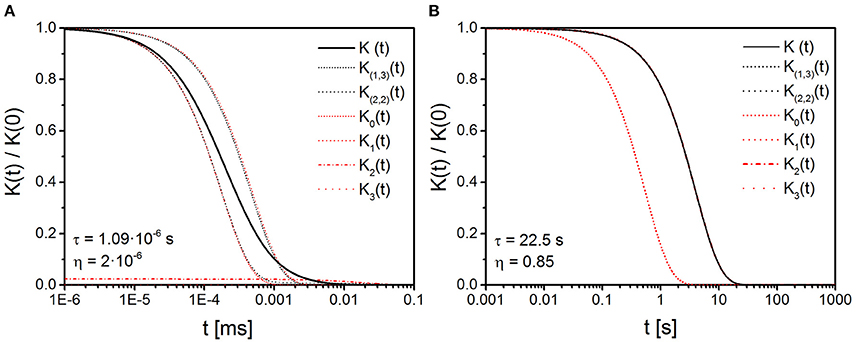
Figure 6. Mono- and bi-exponential approximation in the GMA for nanoparticles and lung tissue. (A) Mono- and bi-exponential approximations are compared to the correlation function K(t) [solid line, obtained from Equation (14)]; parameter set obtained from Muller et al. [52], see also main text. For this extremely short correlation time τ, the monoexponential approximations K₀(t) and K₁(t) coincide with the biexponential approximations K_{(2, 2)}(t) and K_{(1, 3)}(t), respectively. (B) Mono- and bi-exponential approximations for peripheral lung tissue, based on parameters given in Stone et al. [53] and Baete et al. [54]. In this case of a very long correlation time τ, most approximations coincide with K(t).

Recently, it could be shown that Carr-Purcell-Meiboom-Gill (CPMG) relaxation rates are connected to the correlation function [16, 59]. Therefore, knowledge of the correlation function allows obtaining microstructural parameters through CPMG measurements for accumulations of similarly shaped subvoxel structures, for example in the case of lung alveoli [60], microscopic blood products around or in malign cerebral tumors or for microvascular changes in skeletal muscle tissue [21]. Also, based on a recently developed measurement method, magnetic field correlation imaging has been shown promising in its potential to evaluate iron-associated neuropathologies [18, 19]. Knowledge of the exact time course and limit case behavior of the correlation function will aid in further application of magnetic field correlation imaging to determine microstructural parameters of susceptibility gradient based local magnetic field inhomogeneities.

Author Contributions

This work was carried out by the seven authors, in collaboration. CZ designed research; CZ, FK, LB, and TK performed research; CZ and FK contributed numerical tools; and FK, TK, LB, HS, MB, SH, and CZ wrote the paper. Moreover, all authors have read and approved the final manuscript.

Funding

This work was supported by grants from the Deutsche Forschungsgemeinschaft (DFG ZI 1295/2-1 and DFG KU 3555/1-1). FK was also supported by a postdoctoral fellowship from the medical faculty of Heidelberg University and the Hoffmann-Klose Foundation (Heidelberg University).

Conflict of Interest Statement

The authors declare that the research was conducted in the absence of any commercial or financial relationships that could be construed as a potential conflict of interest.

References

1. Haacke EM, Xu Y, Cheng YC, Reichenbach JR. Susceptibility weighted imaging (SWI). Magn Reson Med. (2004) 52:612–8. doi: 10.1002/mrm.20198

PubMed Abstract | CrossRef Full Text | Google Scholar

2. Haacke EM, Tang J, Neelavalli J, Cheng YC. Susceptibility mapping as a means to visualize veins and quantify oxygen saturation. J Magn Reson Imaging (2010) 32:663–76. doi: 10.1002/jmri.22276

PubMed Abstract | CrossRef Full Text | Google Scholar

3. Bartzokis G, Tishler TA, Lu PH, Villablanca P, Altshuler LL, Carter M, et al. Brain ferritin iron may influence age- and gender-related risks of neurodegeneration. Neurobiol Aging (2007) 28:414–23. doi: 10.1016/j.neurobiolaging.2006.02.005

PubMed Abstract | CrossRef Full Text | Google Scholar

4. Richards JM, Shaw CA, Lang NN, Williams MC, Semple SI, MacGillivray TJ, et al. In vivo mononuclear cell tracking using superparamagnetic particles of iron oxide: feasibility and safety in humans. Circ Cardiovasc Imaging (2012) 5:509–17. doi: 10.1161/CIRCIMAGING.112.972596

PubMed Abstract | CrossRef Full Text | Google Scholar

5. Bendszus M, Stoll G. Caught in the act: in vivo mapping of macrophage infiltration in nerve injury by magnetic resonance imaging. J Neurosci. (2003) 23:10892–6.

PubMed Abstract | Google Scholar

6. Ahrens ET, Bulte JW. Tracking immune cells in vivo using magnetic resonance imaging. Nat Rev Immunol. (2013) 13:755–63. doi: 10.1038/nri3531

PubMed Abstract | CrossRef Full Text | Google Scholar

7. Ogawa S, Lee TM, Kay AR, Tank DW. Brain magnetic resonance imaging with contrast dependent on blood oxygenation. Proc Natl Acad Sci USA. (1990) 87:9868–72.

PubMed Abstract | Google Scholar

8. Knight MJ, Kauppinen RA. Diffusion-mediated nuclear spin phase decoherence in cylindrically porous materials. J Magn Reson. (2016) 269:1–12. doi: 10.1016/j.jmr.2016.05.007

PubMed Abstract | CrossRef Full Text | Google Scholar

9. Palombo M, Gentili S, Bozzali M, MacAluso E, Capuani S. New insight into the contrast in diffusional kurtosis images: does it depend on magnetic susceptibility? Magn Reson Med. (2015) 73:2015–24. doi: 10.1002/mrm.25308

PubMed Abstract | CrossRef Full Text | Google Scholar

10. Palombo M, Gabrielli A, De Santis S, Capuani S. The γ parameter of the stretched-exponential model is influenced by internal gradients: validation in phantoms. J Magn Reson. (2012) 216:28–36. doi: 10.1016/j.jmr.2011.12.023

PubMed Abstract | CrossRef Full Text | Google Scholar

11. GadElkarim JJ, Magin RL, Meerschaert MM, Capuani S, Palombo M, Kumar A, et al. Fractional order generalization of anomalous diffusion as a multidimensional extension of the transmission line equation. IEEE J Emerg Sel Topics Circuits Syst. (2013) 3:432–41. doi: 10.1109/JETCAS.2013.2265795

CrossRef Full Text | Google Scholar

12. Yablonskiy DA, Haacke EM. Theory of NMR signal behavior in magnetically inhomogeneous tissues: the static dephasing regime. Magn Reson Med. (1994) 32:749–63.

PubMed Abstract | Google Scholar

13. Ziener CH, Bauer WR, Jakob PM. Transverse relaxation of cells labeled with magnetic nanoparticles. Magn Reson Med. (2005) 54:702–6. doi: 10.1002/mrm.20634

PubMed Abstract | CrossRef Full Text | Google Scholar

14. Kurz FT, Kampf T, Heiland S, Bendszus M, Schlemmer HP, Ziener CH. Theoretical model of the single spin-echo relaxation time for spherical magnetic perturbers. Magn Reson Med. (2014) 71:1888–95. doi: 10.1002/mrm.25196

PubMed Abstract | CrossRef Full Text | Google Scholar

15. Ziener CH, Kurz FT, Kampf T. Free induction decay caused by a dipole field. Phys Rev E Stat Nonlin Soft Matter Phys. (2015) 91:032707. doi: 10.1103/PhysRevE.91.032707

PubMed Abstract | CrossRef Full Text | Google Scholar

16. Jensen JH, Chandra R. NMR relaxation in tissues with weak magnetic inhomogeneities. Magn Reson Med. (2000) 44:144–56. doi: 10.1002/1522-2594(200007)44:1<144::AID-MRM21>3.0.CO;2-O

PubMed Abstract | CrossRef Full Text | Google Scholar

17. Cowan B. Nuclear Magnetic Resonance and Relaxation. Cambridge: Cambridge University Press (1997).

Google Scholar

18. Jensen JH, Chandra R, Ramani A, Lu H, Johnson G, Lee SP, et al. Magnetic field correlation imaging. Magn Reson Med. (2006) 55:1350–61. doi: 10.1002/mrm.20907

PubMed Abstract | CrossRef Full Text | Google Scholar

19. Jensen JH, Szulc K, Hu C, Ramani A, Lu H, Xuan L, et al. Magnetic field correlation as a measure of iron-generated magnetic field inhomogeneities in the brain. Magn Reson Med. (2009) 61:481–5. doi: 10.1002/mrm.21823

PubMed Abstract | CrossRef Full Text | Google Scholar

20. Cho H, Song YQ. NMR measurement of the magnetic field correlation function in porous media. Phys Rev Lett. (2008) 100:025501. doi: 10.1103/PhysRevLett.100.025501

PubMed Abstract | CrossRef Full Text | Google Scholar

21. Kurz FT, Kampf T, Buschle LR, Heiland S, Schlemmer HP, Bendszus M, et al. CPMG relaxation rate dispersion in dipole fields around capillaries. Magn Reson Imaging (2016) 34:875–88. doi: 10.1016/j.mri.2016.03.016

PubMed Abstract | CrossRef Full Text | Google Scholar

22. Kurz FT, Buschle LR, Kampf T, Zhang K, Schlemmer HP, Heiland S, et al. Spin dephasing in a magnetic dipole field around large capillaries: approximative and exact results. J Magn Reson. (2016) 273:83–97. doi: 10.1016/j.jmr.2016.10.012

PubMed Abstract | CrossRef Full Text | Google Scholar

23. Ziener CH, Bauer WR, Melkus G, Weber T, Herold V, Jakob PM. Structure-specific magnetic field inhomogeneities and its effect on the correlation time. Magn Reson Imaging. (2006) 24:1341–7. doi: 10.1016/j.mri.2006.08.005

PubMed Abstract | CrossRef Full Text | Google Scholar

24. Kennan RP, Zhong J, Gore JC. Intravascular susceptibility contrast mechanisms in tissues. Magn Reson Med. (1994) 31:9–21.

PubMed Abstract | Google Scholar

25. Ziener CH, Kampf T, Herold V, Jakob PM, Bauer WR, Nadler W. Frequency autocorrelation function of stochastically fluctuating fields caused by specific magnetic field inhomogeneities. J Chem Phys. (2008) 129:014507. doi: 10.1063/1.2949097

PubMed Abstract | CrossRef Full Text | Google Scholar

26. Ayant Y, Belorizky E, Aluzon J, Gallice J. Calcul des densités spectrales résultant d'un mouvement aléatoire de translation en relaxation par interaction dipolaire magnétique dans les liquides. J Phys France (1975) 36:991–1004.

Google Scholar

27. Sukstanskii AL, Yablonskiy DA. Gaussian approximation in the theory of MR signal formation in the presence of structure-specific magnetic field inhomogeneities. Effects of impermeable susceptibility inclusions. J Magn Reson. (2004) 167:56–67. doi: 10.1016/j.jmr.2003.11.006

PubMed Abstract | CrossRef Full Text | Google Scholar

28. Oppenheim J, Schuler KE, Weiss GH. Stochastic Processes in Chemical Physics. Cambridge: MIT (1977).

Google Scholar

29. Wallace MI, Ying L, Balasubramanian S, Klenerman D. Non-Arrhenius kinetics for the loop closure of a DNA hairpin. Proc Natl Acad Sci USA. (2001) 98:5584–9. doi: 10.1073/pnas.101523498

PubMed Abstract | CrossRef Full Text | Google Scholar

30. Nadler W, Schulten K. Generalized moment expansion for Brownian relaxation processes. J Chem Phys. (1985) 82:151–60.

Google Scholar

31. Bauer HU, Schulten K, Nadler W. Generalized moment expansion of dynamic correlation functions in finite Ising systems. Phys Rev B Condens Matter (1988) 38:445–58.

PubMed Abstract | Google Scholar

32. Noriega JM, Pesquera L, Rodrguez MA. Generalized-moment-expansion method for intensity correlation functions of the single-mode laser. Phys Rev A (1991) 44:6087–91.

PubMed Abstract | Google Scholar

33. Nadler W, Schulten K. Mean relaxation time approximation for dynamical correlation functions in stochastic systems near instabilities. Z Phys B (1988) 72:535–43.

Google Scholar

34. Salomir R, de Senneville BD, Moonen CTW. A fast calculation method for magnetic field inhomogeneity due to an arbitrary distribution of bulk susceptibility. Concepts Magn Reson B (2003) 19B:26. doi: 10.1002/cmr.b.10083

CrossRef Full Text | Google Scholar

35. Mittal S, Wu Z, Neelavalli J, Haacke EM. Susceptibility-weighted imaging: technical aspects and clinical applications, part 2. Am J Neuroradiol. (2009) 30:232–52. doi: 10.3174/ajnr.A1400

PubMed Abstract | CrossRef Full Text | Google Scholar

36. Hudlická, O. Development and adaptability of microvasculature in skeletal muscle. J Exp Biol. (1985) 115:215–28.

PubMed Abstract | Google Scholar

37. Bauer WR, Nadler W, Bock M, Schad LR, Wacker C, Hartlep A, et al. The relationship between the BOLD-induced T2 and T2^*: a theoretical approach for the vasculature of myocardium. Magn Reson Med. (1999) 42:1004–10.

PubMed Abstract | Google Scholar

38. Bauer WR, Schulten K. Nuclear spin dynamics (l=1/2) under the influence of random perturbation fields in the “strong collision approximation”. Berichte der Bunsengesellschaft - Phys Chem Chem Phys. (1992) 96:721–7.

Google Scholar

39. Nadler W, Huang T, Stein DL. Random walks on random partitions in one dimension. Phys Rev E (1996) 54:4037–47.

PubMed Abstract | Google Scholar

40. Krogh A. The supply of oxygen to the tissues and the regulation of the capillary circulation. J Physiol. (1919) 52:457–74.

PubMed Abstract | Google Scholar

41. Hwang LP, Freed JH. Dynamic effects of pair correlation functions on spin relaxation by translational diffusion in liquids. J Chem Phys. (1975) 63:4017.

Google Scholar

42. Ziener CH, Glutsch S, Jakob PM, Bauer WR. Spin dephasing in the dipole field around capillaries and cells: numerical solution. Phys Rev E (2009) 80:046701. doi: 10.1103/PhysRevE.80.046701

PubMed Abstract | CrossRef Full Text | Google Scholar

43. Nadler W, Schulten K. Generalized moment expansion for the Mössbauer spectrum of brownian particles. Phys Rev Lett. (1983) 51:1712–5.

Google Scholar

44. Brünger A, Peters R, Schulten K. Continuous fluorescence microphotolysis to observe lateral diffusion in membranes: theoretical methods and applications. J Chem Phys. (1985) 82:2147–60.

Google Scholar

45. Baker GA, Morris PG. Padé Approximants I, II. Reading MA: Addison-Wesley (1981).

46. Schulten K, Brünger A, Nadler W, Schulten Z. Synergetics - From Microscopic to Macroscopic Order. New York NY: Springer (1984).

47. Barsky D, Pütz B, Schulten K. Theory of heterogeneous relaxation in compartmentalized tissues. Magn Reson Med. (1997) 37:666–75.

PubMed Abstract | Google Scholar

48. Koenig J. Ueber die Integration simultaner Systeme partieller Differentialgleichungen mit mehreren unbekannten Functionen. Math Ann. (1884) 23:520–6.

Google Scholar

49. Householder AS. The Numerical Treatment of a Single Nonlinear Equation. New York, NY: McGraw-Hill (1970).

Google Scholar

50. Jensen JH, Chandra R, Yu H. Quantitative model for the interecho time dependence of the CPMG relaxation rate in iron-rich gray matter. Magn Reson Med. (2001) 46:159–65. doi: 10.1002/mrm.1171

PubMed Abstract | CrossRef Full Text | Google Scholar

51. Brooks RA, Vymazal J, Bulte JW, Baumgarner CD, Tran V. Comparison of T2 relaxation in blood, brain, and ferritin. J Magn Reson Imaging (1995) 5:446–50.

PubMed Abstract | Google Scholar

52. Muller RN, Gillis P, Moiny F, Roch A. Transverse relaxivity of particulate MRI contrast media: from theories to experiments. Magn Reson Med. (1991) 22:178–82.

PubMed Abstract | Google Scholar

53. Stone KC, Mercer RR, Freeman BA, Chang LY, Crapo JD. Distribution of lung cell numbers and volumes between alveolar and nonalveolar tissue. Am Rev Respir Dis. (1992) 146:454–6.

PubMed Abstract | Google Scholar

54. Baete SH, De Deene Y, Masschaele B, De Neve W. Microstructural analysis of foam by use of NMR R2 dispersion. J Magn Reson. (2008) 193:286–96. doi: 10.1016/j.jmr.2008.05.010

PubMed Abstract | CrossRef Full Text | Google Scholar

55. Lauwers F, Cassot F, Lauwers-Cances V, Puwanarajah P, Duvernoy H. Morphometry of the human cerebral cortex microcirculation: general characteristics and space-related profiles. Neuroimage (2008) 39:936–48. doi: 10.1016/j.neuroimage.2007.09.024

PubMed Abstract | CrossRef Full Text | Google Scholar

56. Dickson JD, Ash TW, Williams GB, Sukstanskii AL, Ansorge RE, Yablonskiy DA. Quantitative phenomenological model of the BOLD contrast mechanism. J Magn Reson. (2011) 212:17–25. doi: 10.1016/j.jmr.2011.06.003

PubMed Abstract | CrossRef Full Text | Google Scholar

57. Jensen JH, Chandra R. MR imaging of microvasculature. Magn Reson Med. (2000) 44:224–30. doi: 10.1002/1522-2594(200008)44:2<224::AID-MRM9>3.0.CO;2-M

PubMed Abstract | CrossRef Full Text | Google Scholar

58. Ziener CH, Kampf T, Kurz FT. Diffusion propagators for hindered diffusion in open geometries. Concepts Magn Reson Part A (2015) 44:150–9. doi: 10.1002/cmr.a.21346

CrossRef Full Text | Google Scholar

59. Ziener CH, Kampf T, Jakob PM, Bauer WR. Diffusion effects on the CPMG relaxation rate in a dipolar field. J Magn Reson. (2010) 202:38–42. doi: 10.1016/j.jmr.2009.09.016

PubMed Abstract | CrossRef Full Text | Google Scholar

60. Kurz FT, Kampf T, Buschle LR, Schlemmer HP, Heiland S, Bendszus M, et al. Microstructural analysis of peripheral lung tissue through CPMG inter-echo time R2 dispersion. PLoS ONE (2015) 10:e0141894. doi: 10.1371/journal.pone.0141894

PubMed Abstract | CrossRef Full Text | Google Scholar

61. Ziener CH, Kampf T, Melkus G, Herold V, Weber T, Reents G, et al. Local frequency density of states around field inhomogeneities in magnetic resonance imaging: effects of diffusion. Phys Rev E (2007) 76:031915. doi: 10.1103/PhysRevE.76.031915

PubMed Abstract | CrossRef Full Text | Google Scholar

62. Kampf T, Helluy X, Gutjahr FT, Winter P, Meyer CB, Jakob PM, et al. Myocardial perfusion quantification using the T₁-based FAIR-ASL method: the influence of heart anatomy, cardiopulmonary blood flow and look-locker readout. Magn Reson Med. (2014) 71:1784–97. doi: 10.1002/mrm.24843

PubMed Abstract | CrossRef Full Text | Google Scholar

63. Buschle LR, Kurz FT, Kampf T, Triphan SM, Schlemmer HP, Ziener CH. Diffusion-mediated dephasing in the dipole field around a single spherical magnetic object. Magn Reson Imaging (2015) 33:1126–45. doi: 10.1016/j.mri.2015.06.001

PubMed Abstract | CrossRef Full Text | Google Scholar

Appendices

Appendix A

To determine the eigenvalues in Equation (17), we must find the roots of the function

$\begin{array}{cc}f({\kappa }_n)=j_2^{\prime }({\kappa }_n)y_2^{\prime }\left(\frac{{\kappa }_n}{\sqrt[3]{\eta }}\right)-j_2^{\prime }\left(\frac{{\kappa }_n}{\sqrt[3]{\eta }}\right)y_2^{\prime }({\kappa }_n).& \left(\text{A1}\right)\end{array}$

The derivatives of the spherical Bessel functions j₂ and y₂ can be expanded in a Taylor series for small arguments of κ_n and, thus, an expression for small arguments of f(κ_n) is given as

$\begin{array}{cc}f({\kappa }_n)\approx \frac{6}{5}\frac{1}{{\kappa }_n^3}[{\eta }^{\frac{4}{3}}-{\eta }^{-\frac{1}{3}}]+\frac{18[1-{\eta }^{\frac{5}{3}}]-7{\eta }^{\frac{2}{3}}[1-\eta ]}{105{\kappa }_n\eta }.& \left(\text{A}2\right)\end{array}$

The first zero of Equation (A1) then approximates the first zero of Equation (17) as

$\begin{array}{cc}{\kappa }_1^2\approx \frac{126{\eta }^{\frac{2}{3}}[1-{\eta }^{\frac{5}{3}}]}{18[1-{\eta }^{\frac{7}{3}}]-7{\eta }^{\frac{2}{3}}[1-\eta ]},& \left(\text{A}3\right)\end{array}$

see also Figure 3 and Equation (A16) in Ziener et al. [61].

Appendix B

In the monoexponential approximation (N = 1) or (1, 1)-GMA, only two generalized moments have to be taken into account and Equation (33) reduces to

$\begin{array}{cc}\begin{array}{l}{f}_{(N_h,N_l),1}{\Gamma }_{(N_h,N_l),1}^m={\mu }_m,\text{with}\\ m=-N_l,-N_l+1.\end{array}& \left(\text{B}1\right)\end{array}$

The first ratio τμ₀/μ₋₁ = τ/τ₋₁ is determined in the (1, 1)-GMA that can be regarded as the “mean correlation time approximation,” since, for m = −1, 0, f_{(1, 1)} = μ₀, Γ_{(1, 1)} = 1/τ₋₁ and with Equation (27)

$\begin{array}{cc}{\tau }_{-1}={\displaystyle {\int }_0^{\infty }\text{d}}t\frac{K(t)}{K(0)}={\displaystyle {\int }_0^{\infty }\text{d}}tt{P}_c(t),& \left(\text{B}2\right)\end{array}$

where P_c(t) = −∂_tK(t)/K(0) and τ₋₁ represents a “mean correlation time.” This is in analogy to the “mean relaxation time approximation” in nuclear spin dephasing [38, 62]. While considering the two high-frequency moments μ₀ and μ₁, the corresponding (2, 0)-GMA with f_{(2, 0)} = μ₀ and Γ_{(2, 0)} = μ₁/μ₀ = 1/τ₀ describes the short time behavior of K(t) whereas the (0, 2)-GMA with the two low-frequency moments μ₋₂ and μ₋₁ and parameters $f_{(0,2)}={\mu }_{-1}^2/{\mu }_{-2}$ and Γ_{(0, 2)} = μ₋₁/μ₋₂ = 1/τ₋₂ is a measure for the long time behavior. Since the MCTA is an approximation of the dynamic monoexponentially decaying correlation function, the deviation in Figure 3 of the first ratio τ/τ₋₁ reflects a strongly decaying non-exponential correlation function.

It is useful to define monoexponential functions K_i(t) for arbitrary successive moments as

$\begin{array}{cc}{K}_i(t)=\frac{{\mu }_{1-i}^i}{{\mu }_{-i}^{i-1}}{\text{e}}^{-t\frac{{\mu }_{1-i}}{{\mu }_{-i}}},& \left(\text{B}3\right)\end{array}$

where the index i = 1 uses only the lowest high and low frequency moment and indices i ≤ 0 only high and indices i ≥ 2 only low frequency moments, respectively. In Figures 4A, 5A, the time evolution of the functions K_i(t) is exemplified for both spherical and cylindrical objects, respectively (see below). With Koenig's theorem we find that ${\text{lim}}_{i\to \infty }{K}_i(t)=K_{\mathrm{\text{L}}}(t)$ where K_L is given in Equation (20).

Appendix C

The relaxivity of particulate MR contrast media was examined in Muller et al. [52] to obtain the set of approximate parameters R_i = 50nm, δω = 34·10⁶s⁻¹, η = 2·10⁻⁶, D = 2.3·10⁻⁹m²s⁻¹, and τ = 1.09·10⁻⁶s for iron-oxide nanoparticle suspensions. This extreme example of a very short correlation time was chosen to demonstrate the coincidence of mono- and bi-exponential approximations of the correlation function, as shown in Figure 6A. The biexponential approximations K_{(1, 3)}(t) and K_{(2, 2)}(t) then practically coincide with the respective monoexponential approximations K₁(t) and K₀(t), as anticipated.

The influence of magnetic susceptibility properties of peripheral lung tissue with near-spherical air-containing alveoli on MR signal decay was examined recently, see e.g. [60, 63]. For a typical set of parameters with R_i = 150 μm, δω = 1500 s⁻¹, η = 0.85, D = 1·10⁻⁹m²s⁻¹ (τ = 22.5 s) [53, 54], the correlation function K(t) is shown with mono- and bi-exponential approximations in Figure 6B. In this case of a very long correlation time, mono- and bi-exponential approximations coincide completely with the numerically obtained correlation function K(t), with the exception of K₀(t).