Non-equilibrium Annealed Damage Phenomena: A Path Integral Approach

Introduction

One of the most important aspects in the modern theory of damage phenomena is the possibility to describe damage occurrence on the base of the formalism of statistical physics. Many approaches have been developed [1–24], and surveys of developments can be found in [25–30]. However, the majority of these studies are devoted to equilibrium or near-equilibrium damage occurrence. In our study, we consider a non-equilibrium damage process (a cascade, an avalanche) far from the point of a quasi-static state.

Once the analogy between damage mechanics and statistical physics had been discovered, it immediately became clear that any damage phenomenon can be described as a phase transition, where damage growth represents the appearance of another phase and the point of material failure is the point of the phase transition. The best way to illustrate this similarity is to compare the phase diagrams in Figure 1. There are debates in the literature [3–13, 21, 22, 24, 29–35] about whether this phase transition is of the first order or of the continuous order. The reason for this uncertainty is that spinodal points are very similar to critical points in the sense that in their vicinity a system switches its behavior from the laws intrinsic only to this particular system to universal power-law scaling. However, there is no doubt that any structure under load is in the metastable state since there always exists a nucleus of the critical size. In other words, by breaking enough of the material with external forces, we can always cause material failure. This is a clear indication of metastability, because there is no critical nucleus (no matter how big it is) for stable states.

FIGURE 1

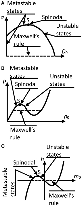
Figure 1. Phase diagrams of (A) a damage phenomenon, (B) a liquid-gas system, and (C) a magnetic system.

To discuss our approach, we involve the fiber-bundle model (further, FBM) as the most illustrative representative of models with damage. However, the applicability of the approach we develop lies beyond the one-dimensional formulation of the FBM and can be easily generalized to two or three-dimensional damage phenomena.

For all possible approaches, an analogy between statistical physics and damage phenomena should rely on mapping of one type of fluctuations on another. In this sense, damage exhibits more complex behavior than classical thermodynamic systems of statistical physics due to the presence of two different forms of disorder: quenched and annealed. Therefore, to perform the aforementioned mapping, these two forms of disorder are usually studied apart from one another.

The influence of quenched disorder on the model behavior is generally observed where the dynamical timescale of fracture is much faster than the timescale of fluctuations. In this case, “frozen” initial disorder in a model plays the crucial role. This type of disorder, employed in the FBM, has been studied by many authors [8, 16, 28, 29, 31–85]. In particular, in our previous studies [21, 22, 30], we introduced quenched disorder by means of the fiber strength variability and for the ensemble of constant strain we were able to map the fluctuations observed on thermodynamic fluctuations in statistical physics.

Another type of behavior is exhibited when a FBM is influenced by the annealed disorder. One of two approaches is generally employed: the disorder is introduced in the model formulation either by means of a phenomenological rate of fiber failures with time [29, 86–109] or by the direct input of a stochastic or thermal noise into the state of stress of a fiber [23, 110–118].

Annealed disorder generates fluctuations which are closely related to their thermodynamic analogs in statistical physics. Indeed, adding stochastic noise to a fiber load seems to be quite similar to the statistical fluctuations of, for example, gas pressure acting on a piston. However, as it was recently discovered [119–123], annealed fluctuations in damage phenomena exceed thermodynamic fluctuations by orders of magnitude. In particular, it was found that the effective temperature required to provide the annealed behavior observed in experiments is 10 times higher (about 3,000 K) than the real temperature during the tests. This discrepancy is explained by complex interactions of quenched and annealed types of disorder which are present simultaneously in the model [18, 113–118, 122, 124].

In our study, we continue our previous research [23, 125, 126] and investigate a FBM with annealed damage evolution. In Section Model, we introduce models which we will use to illustrate our approach. In Section The Classical Gibbs Approach of States, we develop an analog of the classical Gibbs approach for non-equilibrium states. However, this approach has its restrictions which we discuss in Section Restrictions of the Classical Gibbs Approach of States. In Section Statistical Mechanics of the Path Integral Approach, we consider a path integral, when instead of non-equilibrium states of the system we investigate non-equilibrium paths. We map fluctuations of damage on the main concepts of statistical mechanics, such as temperature, entropy, free energy potential, and the law of conservation of energy. However, we find that these concepts are no longer associated with the energy characteristics of the states of the system but are defined over the space of all possible paths. Also, we investigate the behavior of fluctuations for this approach and find “actual” order parameters which diagonalize the matrix of the probability distribution. In the conclusions, we discuss how our theory leads to the description of non-equilibrium phase transitions.

Model

Damage is a complex phenomenon. The basic principles of damage are often completely disguised by the secondary side effects of its appearance. Therefore, to investigate the main concepts of non-equilibrium behavior, it is reasonable to consider initially a simple model.

In this paper, as an illustration, we consider an annealed FBM. We assume that the number N of fibers in the model is constant and infinite in the thermodynamic limit. Intact fibers all carry the same strain ε_f which is identically equal to the strain ε of the total model: ε_f ≡ ε. The stress of each intact fiber is assumed to have a linear elastic dependence on the strain until a fiber failure: σ_f = Eε_f. In this paper, we consider constant strain ε = const as an external boundary constraint of the model. The case of constant stress can be considered in a similar way (the redistribution of the load complicates the analytical solution but does not change the applicability of the path integral). The Young modulus E here is assumed to be the same for all fibers; however, the stress-strain dependence for the total model is non-linear because of fiber failures. We introduce an “intact” order parameter L as the fraction of intact fibers (unity minus the damage parameter). Everywhere further we assume that at the initial time t = 0 all fibers are intact: L_{t = 0} = 1.

As a first modification of the FBM, we consider an annealed fiber-bundle model with noise [23, 110–118] (further, NFBM). Each fiber has thermal fluctuations of its energy characteristics. From statistical mechanics, we know that a piston, which works as a gas boundary and is supported by a spring, has oscillations due to the equipartition of energy. In particular, the elastic energy of the spring fluctuates as if a white Gaussian noise were added to the stress of the spring. Similarly, we assume that the stress of each fiber σ_f has an addition Δσ_f of a white Gaussian noise with zero mean and standard deviation $\sqrt{k_{B}T}$. As it was discussed in Section Introduction, the temperature here may not correspond to the temperature during the experiment but may be several orders higher [119–123].

The probability density function of the noise is

$\begin{array}{ll}p(\Delta {\sigma }_f)=\frac{1}{\sqrt{2\pi k_{B}T}}{e}^{-\frac{\Delta {\sigma }^2}{2k_{B}T}}& (1)\end{array}$

and the cumulative distribution function is

$\begin{array}{ll}P(\Delta {\sigma }_f)=\frac{1}{\sqrt{2\pi k_{B}T}}{\displaystyle \underset{-\infty }{\overset{\Delta {\sigma }_f}{\int }}}{e}^{-\frac{x^2}{2k_{B}T}}dx.& (2)\end{array}$

Each fiber has an a priori assigned strength threshold s which we choose to be the same for all fibers and not to change during the model evolution. A fiber can break only when its stress σ_f = Eε + Δσ_f exceeds its strength s. We consider discrete time-steps dt of the model evolution. At each time-step, the probability of a fiber breaking is 1 − P(s − Eε) and the probability of a fiber staying intact is P(s − Eε). Here we assume that there are no correlations of noise among adjacent fibers. Also, in spite of the fact that the time interval dt between the consecutive time-steps is assumed to be small, it is supposed to be much larger than the duration of any noise correlations. Therefore, we assume that there are no correlations of the noise in time either. Another assumption we utilize is that although the time interval between consecutive time-steps has zero limit, the thermodynamic limit of infinite number of fibers N → +∞ is taken first. Therefore, although only the small fraction of fibers breaks at each time-step, the number of broken fibers is much higher than unity.

Although, we assume the noise to be Gaussian, this does not play any role in our model due to the fact that s, E, and ε are the same for all fibers as well as for all systems in the ensemble and are some constants. Therefore, the noise value Δσ_break = s − Eε at which fibers break is fixed so that P(s − Eε) and 1 − P(s − Eε) are two constants as well.

The second modification of the FBM which we consider (following the original terminology, a model with “breaking kinetics”) is an annealed decay fiber-bundle model [86–109; further, DFBM]. There is no thermal noise in this model. Instead, each (so far intact) fiber has a priori assigned probability p_fdt of failing during the time interval dt and probability (1 − p_fdt) of staying intact.

Here, p_f is the decay rate which is constant during model evolution. The duration of the time-step dt is considered to be fixed as well. Therefore, p_fdt and (1 − p_fdt) are some constants, as well as 1 − P(s − Eε) and P(s − Eε) respectively, which represent fixed probabilities of a fiber breaking or staying intact during a time-step. In this sense, equating p_fdt and 1 − P(s − Eε), we can map the DFBM on the NFBM. However, some care should be exercised when we say p_fdt = 1 − P(s − Eε). Here, we consider dt to be the duration of the time interval during which the Gaussian noise loses its correlation with the value of the noise at the previous time-step and “switches” to a new value. An illustrative example is the output of the Gaussian random generator which provides a discrete set of uncorrelated i.i.d. numbers. In this sense, the duration of dt is not arbitrary but is dictated by the physical processes responsible for the correlations in the noise. Hence, we cannot say here that the considered probabilities are proportional to dt.

The issue can be illustrated with the aid of extreme statistics. If we observe a fiber during a long time interval τ consisting of N >> 1 time-steps dt, the probability of the fiber staying intact during this time interval is $P^N(s-E\epsilon )=e^{\frac{\tau }{dt}lnP(s-E\epsilon )}$, which is clearly not linear with time. Therefore, our mapping of the NFBM onto the DFBM is introduced only for one time-step. In this sense, we will consider only one of these models (the DFBM for the approach of states at Sections The Classical Gibbs Approach of States and Restrictions of the Classical Gibbs Approach of States, which is more convenient for this as it is a model with a well-known solution; the NFBM for the approach of paths at Section Statistical Mechanics of the Path Integral Approach since it is more illustrative of the generalization to more complex model formulations), assuming, however, that all results are valid for the other model as well.

Before going further, we should clarify that we do not consider the healing of fibers: Once a fiber has broken, it stays broken forever. However, our formalism easily allows healing to be added to the model formulation. We need only, in addition to P(s − Eε) and 1 − P(s − Eε), to introduce the probability of a broken fiber healing. All formulae can be easily generalized for this case as well, but due to the complexity of the results already present for the simpler model, we leave it for further studies.

The Classical Gibbs Approach of States

The classical Gibbs approach is formulated in terms of states. To develop its analog for damage phenomena, we need to give some definitions: what we refer to as a non-equilibrium state (or a fluctuation). In more details, this approach is discussed in [30], Chapter 2.

Let us imagine a FBM where we observe separate fibers. As to a microstate {n} we will refer to a particular microconfiguration when for each fiber of the model we prescribe whether it is intact or broken. For example, for a system with N = 3 fibers, one of the microstates is {x x |} where by two symbols “x,” we denoted that the first two fibers of the model are broken, while the symbol “|” means that the third fiber is still intact. For a model with only three fibers, it is easy to list all the possible microstates: {| | |}, {| | x}, {| x |}, {x | |}, {| x x}, {x | x}, {x x |}, {x x x}.

What is the probability of observing a particular microstate in the ensemble of identical systems? For the DFBM, the solution is well-known as the solution of radioactive decay. The probability of a fiber failing at time t during time interval dt is $e^{-p_{f}t}{p}_{f}dt$ and the probability of a fiber failing before the time t is $\underset{0}{\overset{t}{\int }}{e}^{-p_{f}t}{p}_{f}dt=1-e^{-p_{f}t}$. Therefore, the probability of observing a microstate {n} with L intact and (1 - L) broken fibers at the time t is

$\begin{array}{ll}{w}_{\left\{n\right\}}^{\mathrm{\text{ensemble}}}={(e^{-p_{f}t})}^{NL}{(1-e^{-p_{f}t})}^{N(1-L)}.& (3)\end{array}$

We used here the superscript “ensemble” to emphasize that this probability is dictated by the ensemble considered.

We can rewrite the distribution (Equation 3) as

$\begin{array}{ll}{w}_{\left\{n\right\}}^{\mathrm{\text{ensemble}}}=\frac{1}{Z^{\mathrm{\text{ensemble}}}(t)}{e}^{-NL/T^{eff}(t)}& (4)\end{array}$

where we denoted $T^{eff}(t)\equiv {ln}^{-1}(e^{p_{f}t}-1)$. Formula (4) could become identical to the Gibbs probability distribution if we called T^eff(t) the effective temperature. Then $Z^{\mathrm{\text{ensemble}}}(t)={(1-e^{-p_{f}t})}^{-N}$ plays the role of the partition function of the ensemble as we will prove later in Equations (9–11).

We see that the probability distribution of microstates is Gibbsian with the effective temperature changing with time; this allows us to call our ensemble as being “effectively” canonical. Similar to a thermodynamic system with the limited spectrum (like an Ising model), the effective temperature can be both positive and negative, choosing intact states for fibers in the beginning of the model evolution but switching this choice to broken once at later times.

As to a fluctuation [L] (a macrostate [L]) we will refer to the union of all microstates corresponding to the given value of parameter L: $\left[L\right]\equiv {\displaystyle \bigcup _{\left\{n\right\}:L_{\left\{n\right\}}=L}}\left\{n\right\}$. For example, in the case of a model with three fibers, we observe fluctuation [L = 1/3] when we observe one of the three microstates: {| x x}, {x | x}, or {x x |}. For the model with arbitrary N, the number g_[L] of microstates, corresponding to the fluctuation [L], is called the statistical weight of this fluctuation. It can be found as the combinatorial number of outcomes when we distribute NL intact fibers and N(1 − L) broken fibers among N fibers:

$\begin{array}{ll}{g}_{\left[L\right]}=\frac{N!}{(NL)!(N(1-L))!}.& (5)\end{array}$

To simplify this expression, we apply Stirling's approximation

$\begin{array}{ll}N!\approx {\left(\frac{N}{e}\right)}^N\text{O}(N^{\alpha })& (6)\end{array}$

and in the limit N >> 1 we discard the slow power-law dependence O(N^α) on N in comparison with the fast exponential multiplier (N/e)^N:

$\begin{array}{ll}N!{\approx }_{ln}{\left(\frac{N}{e}\right)}^N.& (7)\end{array}$

The special notation for the logarithmic accuracy, “ ≈_ln,” stands here to denote the accuracy to the order of an arbitrary multiplier with the power-law dependence on N (for detailed examples, see [30], Chapter 2).

Applying Stirling's approximation with the logarithmic accuracy to Equation (5), we find

$\begin{array}{ll}{g}_{\left[L\right]}{\approx }_{ln}{L}^{-NL}{(1-L)}^{-N(1-L)}.& (8)\end{array}$

Let us now prove that $Z^{\mathrm{\text{ensemble}}}(t)={(1-e^{-p_{f}t})}^{-N}$ is indeed the partition function of the ensemble. By definition, the partition function is the sum of exponential functions e ^{− NL/Teff(t)} over all microstates:

$\begin{array}{ll}{Z}^{\mathrm{\text{ensemble}}}(t)\equiv {\displaystyle \sum _{\left\{n\right\}}}{e}^{-N{L}_{\left\{n\right\}}/T^{eff}(t)}& (9)\end{array}$

Grouping microstates by fluctuations [L], since all microstates of the same fluctuation have equal values of L, we can write:

$\begin{array}{ll}{Z}^{\mathrm{\text{ensemble}}}(t)={\displaystyle \sum _{\left[L\right]}}{g}_{\left[L\right]}{e}^{-NL/T^{eff}(t)}.& (10)\end{array}$

Substituting here $T^{eff}(t)\equiv {ln}^{-1}(e^{p_{f}t}-1)$ and the statistical weight from Equation (5), we easily prove the required statement:

$\begin{array}{l}{Z}^{\mathrm{\text{ensemble}}}(t)={\displaystyle \sum _{NL=0}^N}\frac{N!}{(NL)!(N(1-L))!}{\left(\frac{1}{e^{p_{f}t}-1}\right)}^{NL}{1}^{N(1-L)}\\ ={\left(\frac{1}{e^{p_{f}t}-1}+1\right)}^N={(1-e^{-p_{f}t})}^{-N}.& (11)\end{array}$

To find the probability $W_{\left[L\right]}^{\mathrm{\text{ensemble}}}$(t, L) of observing a fluctuation [L] in the ensemble (to observe a system with the given fraction L of intact fibers), we multiply probability (Equations 3, 4) of the corresponding microstates by the number (Equation 8) of these microstates:

$\begin{array}{l}{W}_{\left[L\right]}^{\mathrm{\text{ensemble}}}=g_{\left[L\right]}{w}_{\left\{n\right\}\in \left[L\right]}^{\mathrm{\text{ensemble}}}{\approx }_{ln}{\left(\frac{e^{-p_{f}t}}{L}\right)}^{NL}{\left(\frac{1-e^{-p_{f}t}}{1-L}\right)}^{N(1-L)}.\\ & (12)\end{array}$

To attribute a microstate {n} to a particular fluctuation [L], we will write either {n} ∈ [L] or {n}:L_{n} = L. There is no difference between these two notations, and we will utilize the one that will be more convenient at the moment.

The dependence $W_{\left[L\right]}^{\mathrm{\text{ensemble}}}$ on NL has a very narrow maximum due to the “wrestling” of two exponentially fast dependences: g_[L] and $w_{\left\{n\right\}\in \left[L\right]}^{\mathrm{\text{ensemble}}}$. The absolute width of this maximum is of the order of $\sqrt{N}$ while the relative width is of the order of $1/\sqrt{N}$. The most probable fluctuation (which will be observed most commonly) is determined by the maximum of this probability. Equating the derivative to zero, ${\frac{\partial W_{[L]}^{\text{ensemble}}}{\partial L}|}_0=0\text{}\text{\hspace{0.17em}or\hspace{0.17em}}{\frac{\partial \ln \text{}{W}_{[L]}^{\text{ensemble}}}{\partial L}|}_0=0$, we find the equation of state:

$\begin{array}{ll}{L}_0=e^{-p_{f}t}& (13)\end{array}$

The probability distribution $W_{\left[L\right]}^{\mathrm{\text{ensemble}}}$ is normalized by unity:

$\begin{array}{ll}1={\displaystyle \sum _{\left[L\right]}}{W}_{\left[L\right]}^{\mathrm{\text{ensemble}}}={\displaystyle \sum _{\left[L\right]}}{g}_{\left[L\right]}{w}_{\left\{n\right\}\in \left[L\right]}^{\mathrm{\text{ensemble}}}.& (14)\end{array}$

Let us multiply this equality by the partition function:

$\begin{array}{ll}{Z}^{\mathrm{\text{ensemble}}}\equiv {\displaystyle \sum _{\left\{n\right\}}}{e}^{-N{L}_{\left\{n\right\}}/T^{eff}(t)}={\displaystyle \sum _{\left[L\right]}}{g}_{\left[L\right]}{e}^{-NL/T^{eff}(t)},& (15)\end{array}$

where we have again substituted the sum over microstates {n} by the sum over fluctuations [L]. The number of non-zero terms in this sum is of the order of $\sqrt{N}$ (the width of the maximum of $W_{\left[L\right]}^{\mathrm{\text{ensemble}}}$):

$\begin{array}{ll}{Z}^{\mathrm{\text{ensemble}}}=g_{\left[L_0\right]}{e}^{-N{L}_0/T^{eff}(t)}\text{O}\left(\sqrt{N}\right).& (16)\end{array}$

Applying the logarithmic approximation (neglecting slow power-law dependencies and keeping only fast exponential dependencies), we prove the classical result of statistical mechanics that a partition function equals its maximal term:

$\begin{array}{ll}{Z}^{\mathrm{\text{ensemble}}}{\approx }_{ln}{g}_{\left[L_0\right]}{e}^{-N{L}_0/T^{eff}(t)}.& (17)\end{array}$

Dividing this equation by Z^ensemble, we find another important relationship:

$\begin{array}{ll}{w}_{\left\{n\right\}:L_{\left\{n\right\}}=L_0}^{\mathrm{\text{ensemble}}}{\approx }_{ln}\frac{1}{g_{\left[L_0\right]}}& (18)\end{array}$

that the probability of microstates corresponding to the most probable fluctuation [L₀] is the inversed number of these microstates (the principle of the equivalence between the canonical and microcanonical ensembles).

Equality (Equation 18) can be found without multiplying (Equation 14) by Z^ensemble. Only in this case, we arrive at the equation

$\begin{array}{ll}1=g_{\left[L_0\right]}{w}_{\left\{n\right\}:L_{\left\{n\right\}}=L_0}^{\mathrm{\text{ensemble}}}\text{O}\left(\sqrt{N}\right){\approx }_{ln}{g}_{\left[L_0\right]}{w}_{\left\{n\right\}:L_{\left\{n\right\}}=L_0}^{\mathrm{\text{ensemble}}}& (19)\end{array}$

which states that there are about $\sqrt{N}$ fluctuations under the width of the maximum of $W_{\left[L\right]}^{\mathrm{\text{ensemble}}}$ with the probability similar to the most probable fluctuation [L₀]. Thereby, the probability of [L₀] is of the order of $1/\sqrt{N}$ which returns us to Equation (18).

Let us introduce the partial partition function (of a fluctuation)

$\begin{array}{ll}{Z}_{\left[L\right]}\equiv {\displaystyle \sum _{\left\{n\right\}\in \left[L\right]}}{e}^{-N{L}_{\left\{n\right\}}/T^{eff}(t)}=g_{\left[L\right]}{e}^{-NL/T^{eff}(t)}& (20)\end{array}$

when we sum the exponential functions not over all microstates but only over microstates of the particular fluctuation. Then, probability (Equation 12) of observing the fluctuation is directly related to the partial partition function of this fluctuation:

$\begin{array}{ll}{W}_{\left[L\right]}^{\mathrm{\text{ensemble}}}=g_{\left[L\right]}{w}_{\left\{n\right\}\in \left[L\right]}^{\mathrm{\text{ensemble}}}=\frac{Z_{\left[L\right]}}{{\mathrm{\text{Z}}}^{\mathrm{\text{ensemble}}}}.& (21)\end{array}$

Next, let us consider averaging in the ensemble:

$\begin{array}{l}{\langle f\rangle }^{\mathrm{\text{ensemble}}}\equiv {\displaystyle \sum _{\left\{n\right\}}}{f}_{\left\{n\right\}}{w}_{\left\{n\right\}}^{\mathrm{\text{ensemble}}}={\displaystyle \sum _{\left[L\right]}}{f}_{\left\{n\right\}:L_{\left\{n\right\}}=L}{g}_{\left[L\right]}{w}_{\left\{n\right\}:L_{\left\{n\right\}}=L}^{\mathrm{\text{ensemble}}}\\ ={\displaystyle \sum _{\left[L\right]}}{f}_{\left\{n\right\}:L_{\left\{n\right\}}=L}{W}_{\left[L\right]}^{\mathrm{\text{ensemble}}}.& (22)\end{array}$

As an example, we consider averaging of L:

$\begin{array}{ll}{\langle L\rangle }^{\mathrm{\text{ensemble}}}={\displaystyle \sum _{\left[L\right]}}L{W}_{\left[L\right]}^{\mathrm{\text{ensemble}}}.& (23)\end{array}$

Here the probability distribution $W_{\left[L\right]}^{\mathrm{\text{ensemble}}}$ is the very fast dependence comparing to slow dependence L. Besides, $W_{\left[L\right]}^{\mathrm{\text{ensemble}}}$ is normalized by unity. Therefore, it plays the role of a delta-function δ(L − L₀), and we immediately find:

$\begin{array}{ll}{\langle L\rangle }^{\mathrm{\text{ensemble}}}\approx L_0& (24)\end{array}$

The definition $\left[L\right]\equiv \underset{\left\{n\right\}:L_{\left\{n\right\}}=L}{\bigcup \left\{n\right\}}$ of a fluctuation [L] can be presented in terms of non-equilibrium probability distributions which we developed in details in [30], Chapter 2 as the generalization of the Leontovich approach of non-equilibrium states [127, 128]. We observe a fluctuation [L] when in the ensemble we observe a system with the given fraction L of intact fibers. It is like in statistical physics to observe fluctuations of gas density when, for example, the gas has gathered spontaneously all its molecules in the left half of its volume while there are no molecules in another (right) half of the volume. We call it a fluctuation (a macrostate). But to determine the properties of this state, it is not enough to observe it for a microsecond as a microstate. To study this state, we isolate the gas in the left half of the volume by a virtual boundary and observe for some time before releasing it. But what does this additional isolation mean? It means that the gas visits only the microstates corresponding to our fluctuation and does not visit other microstates.

The same purpose can be achieved by considering non-equilibrium probability distributions [30]. Distribution (Equations 3, 4) is dictated by the ensemble boundary conditions similar to the pressure and temperature dictated by the boundary conditions for the gas. However, a system may disregard these orders and behave independently. Imagine students who are ordered to read one paper a week on average. One student works hard and may read five papers a week on average while another one does not study at all. Similar, a system may fluctuate violating orders from the ensemble. For the gas, it means that the system stays in the left half of its volume (have non-zero probabilities only for those microstates which do not have molecules in the right half). For our system with damage, it means that only those microstates have non-zero probabilities which possess the correct value of the intact fiber fraction L while probabilities of other microstates are zero:

$\begin{array}{ll}{w}_{\left\{n\right\}}=\{\begin{array}{c}1/g_{\left[L\right]},\left\{n\right\}:L_{\left\{n\right\}}=L\\ 0,\left\{n\right\}:L_{\left\{n\right\}}\ne L\\ \end{array}.& (25)\end{array}$

To find the entropy of the fluctuation, we apply Gibbs definition and arrive at Boltzmann's entropy:

$\begin{array}{ll}{S}_{\left[L\right]}\equiv -{\displaystyle \sum _{\left\{n\right\}}}{w}_{\left\{n\right\}}ln{w}_{\left\{n\right\}}=ln{g}_{\left[L\right]}.& (26)\end{array}$

For the equilibrium probability distribution, this transforms into:

$\begin{array}{l}{S}^{\mathrm{\text{ensemble}}}\equiv -{\displaystyle \sum _{\left\{n\right\}}}{w}_{\left\{n\right\}}^{\mathrm{\text{ensemble}}}ln{w}_{\left\{n\right\}}^{\mathrm{\text{ensemble}}}\\ =-{\displaystyle \sum _{\left[L\right]}}{g}_{\left[L\right]}{w}_{\left\{n\right\}}^{\mathrm{\text{ensemble}}}ln{w}_{\left\{n\right\}}^{\mathrm{\text{ensemble}}}\\ =-{\displaystyle \sum _{\left[L\right]}}{W}_{\left[L\right]}^{\mathrm{\text{ensemble}}}ln{w}_{\left\{n\right\}}^{\mathrm{\text{ensemble}}},& (27)\end{array}$

where we have substituted the sum over microstates {n} by the sum over fluctuations [L]. In the right-hand side of Equation (27), the dependence $ln{w}_{\left\{n\right\}}^{\text{ensemble}}$ is a slow, power-law dependence on NL while $W_{\left[L\right]}^{\text{ensemble}}$ is the exponentially fast dependence, acting like a delta-function due to its normalization ${\displaystyle \sum _{\left[L\right]}}{W}_{\left[L\right]}^{\text{ensemble}}=1$. Therefore, utilizing Equation (18), we immediately find Boltzmann's expression for the equilibrium entropy as well:

$\begin{array}{ll}{S}^{\mathrm{\text{ensemble}}}=-ln{w}_{\left\{n\right\}:L_{\left\{n\right\}}=L_0}^{\mathrm{\text{ensemble}}}=ln{g}_{\left[L_0\right]}.& (28)\end{array}$

The non-equilibrium free energy potential (the effective Helmholtz energy) of a fluctuation may be introduced as

$\begin{array}{ll}{F}_{\left[L\right]}\equiv NL-T^{eff}{S}_{\left[L\right]}=-T^{eff}ln{Z}_{\left[L\right]}.& (29)\end{array}$

For the equilibrium free energy we find

$\begin{array}{ll}{F}^{\mathrm{\text{ensemble}}}\equiv N{L}_0-T^{eff}{S}^{\mathrm{\text{ensemble}}}=-T^{eff}ln{Z}^{\mathrm{\text{ensemble}}}.& (30)\end{array}$

Instead of free energy, we can define the action of free energy on a fluctuation (this will remove the asymmetry of temperature; for details, see [30, Section 2.16]):

$\begin{array}{l}{A}_{\left[L\right]}\equiv NL/T^{eff}-S_{\left[L\right]}=-ln{Z}_{\left[L\right]}=-ln\left({\mathrm{\text{Z}}}^{\mathrm{\text{ensemble}}}{W}_{\left[L\right]}^{\mathrm{\text{ensemble}}}\right).\\ & (31)\end{array}$

We see that the action of the free-energy is directly related to the probability distribution of fluctuations and its minimization is equivalent to the evolution from states of low probability to highly probable states.

The ensemble action of free energy is:

$\begin{array}{ll}{A}^{\mathrm{\text{ensemble}}}\equiv N{L}_0/T^{eff}-S^{\mathrm{\text{ensemble}}}=-ln{Z}^{\mathrm{\text{ensemble}}}.& (32)\end{array}$

All other results, generally developed for the canonical ensemble, are applicable here as well (for details, see [30], Chapter 2). However, our purpose in this manuscript is to suggest possible approaches to solve an arbitrary system, not as simple as the DFBM. Therefore, we provided here the classical Gibbs approach of states only to the purpose to highlight differences with the proposed below path integral approach.

Restrictions of the Classical Gibbs Approach of States

In the previous section, we were lucky that our system had an analytical solution. This was the consequence of the fact that we were able to find a priori the probability $\underset{0}{\overset{t}{\int }}{e}^{-p_{f}t}{p}_{f}dt=1-e^{-p_{f}t}$ of a fiber failing before time t. For the case of an arbitrary system, we generally know the distribution of probabilities only for one time-step. In other words, if at time t_i a system with probability $w_{\left\{n_i\right\}}^{\mathrm{\text{ensemble}}}$ is in a microstate {n_i} with NL_i intact fibers, we know that the probability of this system at the next time-step t_i+1 being in a microstate {n_i+1} with NL_i+1 intact fibers is

$\begin{array}{ll}{w}_{\left\{n_{i+1}\right\}}^{\mathrm{\text{ensemble}}}=w_{\left\{n_i\right\}}^{\mathrm{\text{ensemble}}}{\left(1-p_{f}t\right)}^{N{L}_{i+1}}{\left(p_{f}t\right)}^{N(L_i-L_{i+1})}.& (33)\end{array}$

In fact, we utilized here the general Gibbs formula $\frac{d{w}_{\left\{\right\}}^{\text{ensemble}}}{dt}(t)=F\left[w_{\left\{\right\}}^{\text{ensemble}}(t^{\prime }),t^{\prime }\le t\right]$ that the evolution of the distribution of probabilities of microstates is determined by some functional dependence on the history of the model. To obtain the distribution of probabilities of the microstates at time t we have to integrate this equation over all possible paths among all previous configurations [e.g., 129, 130]. We have to integrate all possible intermediate configurations; these configurations are interconnected by the tremendous number of different paths; each path can have its own probability or be prohibited (irreversible damage in the case of the FBM, when a broken fiber cannot become intact again). Therefore, the integration of combinatorial sums becomes cumbersome.

This approach corresponds to the classical Gibbs non-equilibrium statistical mechanics, when microstates of a system are identified with the system's microconfigurations and macrostates of a system are identified with the system's macroconfigurations. However, we know that the probabilities for Markov processes are associated not with the states but with the paths among these states (for the first-order Markov process, the probability of a path A-B-C-D is P (D|C)P(C|B)P(B|A)P(A) while to find the probability of the system arriving after three steps at state D we should have three sums involved: ${\displaystyle \sum _{X_1,X_2,X_3}P\text{}\left(D|X_3\right)\text{}P\left(X_3|X_2\right)\text{}P\left(X_2|X_1\right)\text{}P\text{}\left(X_1\right)}$, see Figure 2). Therefore, it is much easier to find a distribution of the probabilities only for a macrogroup of paths than for all the paths leading to a macrostate. In the Gibbs approach, the states of a system were chosen as bases, although we see that everything points to the fact that as bases we should choose not the states but the paths [125, 126, 131–142]. We will see how we can develop such an approach in the next section. The benefit of this approach will be that its bases will not include integrals of the states for the previous evolution of the system but, in contrast, will be this evolution itself.

FIGURE 2

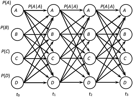
Figure 2. The graph among A, B, C, and D states.

Statistical Mechanics of the Path Integral Approach

In the previous sections and in our previous publications [21, 22, 30], we identified microstates of a system with system's microconfigurations and macrostates of a system with system's macroconfigurations. However, this approach worked well only for equilibrium statistical mechanics. For non-equilibrium statistical mechanics, we should develop another approach [126].

As an illustration, we consider the case of the NFBM and assume that the process consists of ν time intervals of duration dt, from t₀ = 0 to t_ν = ν · dt. For each time-step t_i as an order parameter we choose the value of the intact parameter L_i at this time-step. For the total process the order parameter is the total history of the intact parameter L(t) ≡ L₀,…, L_ν. We assume that the process always starts from zero damage L₀ = 1, so the quantity L₀ will not be variable in the ensemble. We assume that broken fibers cannot become intact again; therefore, increments of the intact parameter ΔL_i ≡ L_i − L_{i − 1} are always negative.

At each time-step t_i, a particular system in the ensemble has its own value of the intact parameter L_i and is in one of the microconfigurations {n_i} corresponding to this intact parameter. The next possible microconfiguration for this system at the time-step t_i+1 can only be a microconfiguration in which all the broken fibers remain broken. This makes our system a Markov process of order 1. For the total process from t₀ = 0 to t_ν = ν · dt, we construct all possible chains of microconfigurations. Each such chain, as a possible sequence of particular microconfigurations {n₀}, {n₁}, …, {n_ν}, will be referred to as a micropath {n₀} → {n₁} → … → {n_ν} (further, we will abbreviate this notation as {n₀} → {n_ν}). For example, for a system with N = 3 fibers, one of possible micropaths is {| | |} → {| x |} → {x x |} → {x x |} → {x x x} where symbol “|” denotes an intact fiber while symbol “x” denotes a broken fiber.

Let us assume that for a micropath {n₀} → {n_ν} the sequence of the configurations has the evolution of the intact parameter L(t) ≡ L₀,…, L_ν. Then the probability of this micropath is

$\begin{array}{l}{w}_{\left\{n_0\right\}\to \left\{n_{\nu }\right\}}^{\mathrm{\text{ensemble}}}={(1-P)}^{N|\Delta L_1|}{P}^{N(L_0-|\Delta L_1|)}\\ \dots {(1-P)}^{N|\Delta L_{\nu }|}{P}^{N(L_{\nu -1}-|\Delta L_{\nu }|)}\\ ={\left(\frac{1-P}{P}\right)}^{N(1-L_{\nu })}{P}^{N{\displaystyle \sum _{i=1}^{\nu }}{L}_{i-1}}& (34)\end{array}$

as the probability of N|ΔL_i| fibers failing and of NL_i ≡ N(L_{i − 1} − |ΔL_i|) fibers staying intact, where P ≡ P(s – Eε) is constant. This probability $w_{\left\{n_0\right\}\to \left\{n_{\nu }\right\}}^{\mathrm{\text{ensemble}}}$ is dictated by the ensemble and, in particular, by the value of P. This constraint is a model input and acts similarly to the temperature prescribed in the canonical ensemble. In the canonical ensemble, an external medium dictates the distribution of the probabilities for different paths but a system actually can be not in equilibrium with the dictated distribution and realizes some other probability distribution w_{{n0} → {nν}} for its paths. Therefore, we used here the abbreviation “ensemble” to emphasize that this probability distribution corresponds to the requirements stated regardless of possible fluctuations.

As to the macropath [L₀] → [L₁] → … → [L_ν] (further, we will abbreviate this notation as [L₀] → [L_ν]) we will refer to a subset of all micropaths {n₀} → {n_ν} corresponding to the specified evolution of the intact parameter L(t): $\left[L_0\right]\to \left[L_{\nu }\right]=\underset{\left\{n_0\right\}\to \left\{n_{\nu }\right\}:L_{\left\{n_i\right\}}=L_i}{\bigcup \left\{n_0\right\}}\to \left\{n_{\nu }\right\}$. For example, for the system with N = 3 fibers macropath [1] → [1/3] → [1/3] → [0] unites micropaths {|||} → {|xx} → {|xx} → {xxx}, {|||} → {x|x} → {x|x} → {xxx}, and {|||} → {xx|} → {xx|} → {xxx}. In fact, macropath states that the system passes during its evolution the prescribed values of L but does not specify particular microstates.

The probabilities of micropaths corresponding to a macropath [L₀] → [L_ν] are all equal one to another and are given by Equation (34); the number of these micropaths is

$\begin{array}{l}{g}_{\left[L_0\right]\to \left[L_{\nu }\right]}=\frac{(N{L}_0)!}{(N|\Delta L_1|)!(N(L_0-|\Delta L_1|))!}.\\ \frac{(N{L}_1)!}{(N|\Delta L_2|)!(N(L_1-|\Delta L_2|))!}.\\ \dots ·\frac{(N{L}_{\nu -1})!}{(N|\Delta L_{\nu }|)!(N(L_{\nu -1}-|\Delta L_{\nu }|))!}& (35)\end{array}$

as a combinatorial choice of N|ΔL_i| failed fibers among NL_i−1 initial fibers. We can cancel (NL_i)! in the numerators and (N(L_{i − 1} - |ΔL_i|))! in the denominators to obtain

$\begin{array}{l}{g}_{\left[L_0\right]\to \left[L_{\nu }\right]}=\frac{(N{L}_0)!}{(N{L}_{\nu })!{\displaystyle \prod _{i=1}^{\nu }}(N|\Delta L_i|)!}{\approx }_{ln}{(L_{\nu })}^{-N{L}_{\nu }}{\displaystyle \prod _{i=1}^{\nu }}|\Delta L_i{|}^{-N|\Delta L_i|},\\ & (36)\end{array}$

where the notation “≈_ln” means that in the thermodynamic limit N → +∞ all power-law multipliers are neglected in comparison with the exponential dependence on N.

The probability of the system having a macropath [L₀] → [L_ν] (to move among macroconfigurations with the specified L(t)) is

$\begin{array}{ll}{W}_{\left[L_0\right]\to \left[L_{\nu }\right]}^{\mathrm{\text{ensemble}}}={\displaystyle \sum _{n=1}^{g_{\left[L_0\right]\to \left[L_{\nu }\right]}}}{w}_{\left\{n_0\right\}\to \left\{n_{\nu }\right\}}^{\mathrm{\text{ensemble}}}=g_{\left[L_0\right]\to \left[L_{\nu }\right]}{w}_{\left\{n_0\right\}\to \left\{n_{\nu }\right\}}^{\mathrm{\text{ensemble}}}.& (37)\end{array}$

Maximization of $W_{\left[L_0\right]\to \left[L_{\nu }\right]}^{\mathrm{\text{ensemble}}}$ over all the possible macropaths gives the most probable macropath L⁽⁰⁾(t):

$\begin{array}{ll}{W}_{\left[L_0^{(0)}\right]\to \left[L_{\nu }^{(0)}\right]}^{\mathrm{\text{ensemble}}}={\displaystyle \underset{L_1,\dots ,L_{\nu }}{max}}{W}_{\left[L_0\right]\to \left[L_{\nu }\right]}^{\mathrm{\text{ensemble}}}.& (38)\end{array}$

Dependence L⁽⁰⁾(t) is the dependence of L which we will observe generally in the ensemble.

The function $W_{\left[L_0\right]\to \left[L_{\nu }\right]}^{\mathrm{\text{ensemble}}}$, given by Equation (37), is the product of g_{[L0] → [Lν]} and $w_{\left\{n_0\right\}\to \left\{n_{\nu }\right\}}^{\mathrm{\text{ensemble}}}$. Both these functions contain exponentially fast dependences on N (N is infinite in the thermodynamic limit). Therefore, in the space of all paths, the function $W_{\left[L_0\right]\to \left[L_{\nu }\right]}^{\mathrm{\text{ensemble}}}$ has a very narrow maximum at the most probable macropath $\left[L_0^{(0)}\right]\to \left[L_{\nu }^{(0)}\right]$. As we will see below, the absolute width of this maximum is proportional to $\sqrt{N}$ while the relative width is proportional to $1/\sqrt{N}$. Therefore, the number of different macropaths [L₀] → [L_ν] under the width of this maximum has a power-law dependence on N while the number g_{[L0] → [Lν]} of micropaths {n₀} → {n_ν} corresponding to each of these macropaths [L₀] → [L_ν] has the exponential dependence on N. Therefore, for the normalization of the function $W_{\left[L_0\right]\to \left[L_{\nu }\right]}^{\mathrm{\text{ensemble}}}$ with the logarithmic accuracy we obtain

$\begin{array}{l}1={\displaystyle \sum _{\left[L_0\right]\to \left[L_{\nu }\right]}}{W}_{\left[L_0\right]\to \left[L_{\nu }\right]}^{\mathrm{\text{ensemble}}}{\approx }_{ln}{W}_{\left[L_0^{(0)}\right]\to \left[L_{\nu }^{(0)}\right]}^{\mathrm{\text{ensemble}}}\\ \equiv g_{\left[L_0^{(0)}\right]\to \left[L_{\nu }^{(0)}\right]}{w}_{\left\{n_0\right\}\to \left\{n_{\nu }\right\}\in \left[L_0^{(0)}\right]\to \left[L_{\nu }^{(0)}\right]}^{\mathrm{\text{ensemble}}}.& (39)\end{array}$

This provides

$\begin{array}{ll}{g}_{\left[L_0^{(0)}\right]\to \left[L_{\nu }^{(0)}\right]}{\approx }_{ln}1/w_{\left\{n_0\right\}\to \left\{n_{\nu }\right\}\in \left[L_0^{(0)}\right]\to \left[L_{\nu }^{(0)}\right]}^{\mathrm{\text{ensemble}}}.& (40)\end{array}$

In other words, the probability of each micropath of the most probable macropath $\left[L_0^{(0)}\right]\to \left[L_{\nu }^{(0)}\right]$ has the order of the inverted number of these micropaths.

Next, let us consider averaging over the space of all possible paths:

$\begin{array}{ll}{\langle f\rangle }^{\mathrm{\text{ensemble}}}(t)\equiv {\displaystyle \sum _{\left\{n_0\right\}\to \left\{n_{\nu }\right\}}}{w}_{\left\{n_0\right\}\to \left\{n_{\nu }\right\}}^{\mathrm{\text{ensemble}}}{f}_{\left\{n_0\right\}\to \left\{n_{\nu }\right\}}.& (41)\end{array}$

As an example, we again consider averaging of L:

$\begin{array}{cc}\begin{array}{l}{\langle L\rangle }^{\text{ensemble}}(t)\equiv {\displaystyle \sum _{\left\{n_0\right\}\to \left\{n_{\nu }\right\}}{L}_{\left\{n_0\right\}\to \left\{n_{\nu }\right\}}{w}_{\left\{n_0\right\}\to \left\{n_{\nu }\right\}}^{\text{ensemble}}}\\ \equiv \{\begin{array}{c}{L}_0,t=t_0\\ {\displaystyle \sum _{\left\{n_0\right\}\to \left\{n_{\nu }\right\}}{L}_{\left\{n_i\right\}}{w}_{\left\{n_0\right\}\to \left\{n_{\nu }\right\}}^{\text{ensemble}}},t=t_i\end{array}=\\ =\{\begin{array}{c}{L}_0,t=t_0\\ {\displaystyle \sum _{[L_0]\to [L_{\nu }]}{g}_{[L_0]\to [L_{\nu }]}{L}_i{w}_{\left\{n_0\right\}\to \left\{n_{\nu }\right\}}^{\text{ensemble}}},t=t_i\end{array}.\end{array}& \left(42\right)\end{array}$

Of course, in the thermodynamic limit, 〈L〉^ensemble(t) coincides with the most probable macropath: 〈L〉^ensemble(t) ≈ L⁽⁰⁾(t).

Probability distribution (Equation 34) is the distribution dictated by the ensemble. However, we can also consider other distributions w_{{n0} → {nν}} which do not obey the ensemble requirements. Next, as a fluctuation we consider the macropath [L₀] → [L_ν]. The number g_{[L0] → [Lν]} of micropaths corresponding to this macropath is given by Equation (36). Again, to observe this macropath, we need to “isolate” our system in this macropath. This is achieved by considering the probability distribution w_{{n0} → {nν}} such that only the micropaths belonging to the considered macropath [L₀] → [L_ν] have non-zero probabilities:

$\begin{array}{ll}{w}_{\left\{n_0\right\}\to \left\{n_{\nu }\right\}}=\{\begin{array}{c}1/g_{\left[L_0\right]\to \left[L_{\nu }\right]},\left\{n_0\right\}\to \left\{n_{\nu }\right\}\in \left[L_0\right]\to \left[L_{\nu }\right]\\ 0,\left\{n_0\right\}\to \left\{n_{\nu }\right\}\notin \left[L_0\right]\to \left[L_{\nu }\right]\\ \end{array}.& (43)\end{array}$

Here we assumed the equiprobability of all micropaths of the system isolated in the macropath. Actually, this may not always be true but depends solely on how we build fluctuations as an instrument of our investigation.

The entropy of the considered macropath is

$\begin{array}{l}{S}_{\left[L_0\right]\to \left[L_{\nu }\right]}\equiv -{\displaystyle \sum _{\left\{n_0\right\}\to \left\{n_{\nu }\right\}}}{w}_{\left\{n_0\right\}\to \left\{n_{\nu }\right\}}ln{w}_{\left\{n_0\right\}\to \left\{n_{\nu }\right\}}=ln{g}_{\left[L_0\right]\to \left[L_{\nu }\right]}.\\ & (44)\end{array}$

We should emphasize here that the entropy introduced is the “dynamical” entropy of the distribution of probabilities for the paths and must not be confused with the classical Gibbs entropy associated with the distribution of probabilities for the states (configurations). In our notations, the classical Gibbs entropy would be $S_{\left\{n\right\}}(t)\equiv -{\displaystyle \sum _{\left\{n\right\}}}{w}_{\left\{n\right\}}(t)ln{w}_{\left\{n\right\}}(t)$ as the average at time t over the probabilities w_{n}(t) of microconfigurations at this time. On the contrary, the path entropy is associated with the probabilities w_{{n0} → {nν}} of micropaths of the total process and cannot be attributed to system's characteristics at a particular time t.

If, instead of the probability distribution w_{{n0} → {nν}}, we consider probability distribution (Equation 34) dictated by the ensemble, for the ensemble path entropy we find:

$\begin{array}{l}{S}^{\mathrm{\text{ensemble}}}\equiv -{\displaystyle \sum _{\left\{n_0\right\}\to \left\{n_{\nu }\right\}}}{w}_{\left\{n_0\right\}\to \left\{n_{\nu }\right\}}^{\mathrm{\text{ensemble}}}ln{w}_{\left\{n_0\right\}\to \left\{n_{\nu }\right\}}^{\mathrm{\text{ensemble}}}\\ =-{\displaystyle \sum _{\left[L_0\right]\to \left[L_{\nu }\right]}}{g}_{\left[L_0\right]\to \left[L_{\nu }\right]}{w}_{\left\{n_0\right\}\to \left\{n_{\nu }\right\}}^{\mathrm{\text{ensemble}}}ln{w}_{\left\{n_0\right\}\to \left\{n_{\nu }\right\}}^{\mathrm{\text{ensemble}}}=\\ =-{\displaystyle \sum _{\left[L_0\right]\to \left[L_{\nu }\right]}}{W}_{\left[L_0\right]\to \left[L_{\nu }\right]}^{\mathrm{\text{ensemble}}}ln{w}_{\left\{n_0\right\}\to \left\{n_{\nu }\right\}}^{\mathrm{\text{ensemble}}}.& (45)\end{array}$

Here, the function $ln{w}_{\left\{n_0\right\}\to \left\{n_{\nu }\right\}}^{\mathrm{\text{ensemble}}}$ has a slow power-law dependence on N in comparison with the functions g_{[L0] → [Lν]} and $w_{\left\{n_0\right\}\to \left\{n_{\nu }\right\}}^{\mathrm{\text{ensemble}}}$ which have exponentially fast dependences on N. Therefore, the dependence $W_{\left[L_0\right]\to \left[L_{\nu }\right]}^{\mathrm{\text{ensemble}}}$ acts as a delta-function around the most probable macropath, and we find:

$\begin{array}{l}{S}^{\mathrm{\text{ensemble}}}\approx -ln{w}_{\left\{n_0\right\}\to \left\{n_{\nu }\right\}\in [L_0^{(0)}]\to [L_{\nu }^{(0)}]}^{\mathrm{\text{ensemble}}}\approx ln{g}_{[L_0^{(0)}]\to [L_{\nu }^{(0)}]}\\ =S_{[L_0^{(0)}]\to [L_{\nu }^{(0)}]}.& (46)\end{array}$

In other words, the entropy of the total ensemble of paths equals the entropy of the most probable macropath.

We can rewrite the equilibrium distribution of probabilities, given by Equation (34), as

$\begin{array}{ll}{w}_{\left\{n_0\right\}\to \left\{n_{\nu }\right\}}^{\mathrm{\text{ensemble}}}=\frac{1}{Z^{\mathrm{\text{ensemble}}}}exp\left(-N{L}_{\nu }/T_{\nu }-N\left({\displaystyle \sum _{i=1}^{\nu }}{L}_{i-1}\right)/T_{\int }\right)& (47)\end{array}$

where $Z^{\mathrm{\text{ensemble}}}={\left(\frac{P}{1-P}\right)}^N$, $T_{\nu }={ln}^{-1}\left\{(1-P)/P\right\}$, and $T_{\int }=-{ln}^{-1}P$. It is easy to see that Z^ensemble is the path partition function of the system: $Z^{\mathrm{\text{ensemble}}}={\displaystyle \sum _{\left\{n_0\right\}\to \left\{n_{\nu }\right\}}}exp\left\{-N{L}_{\nu }/T_{\nu }-N\left({\displaystyle \sum _{i=1}^{\nu }}{L}_{i-1}\right)/T_{\int }\right\}$. T_ν and T_∫ play the roles of effective temperatures. We see that when P is close to unity (the probability of a fiber breaking is small), the temperature T_∫ is infinite but positive.

The definition of the temperature T_ν is, to some extent, ambiguous. Indeed, we can rewrite Equation (34) for probabilities as

$\begin{array}{l}{w}_{\left\{n_0\right\}\to \left\{n_{\nu }\right\}}^{\mathrm{\text{ensemble}}}={(1-P)}^{N|\Delta L_1|}{P}^{N{L}_1}\dots {(1-P)}^{N|\Delta L_{\nu }|}{P}^{N{L}_{\nu }}\\ ={(1-P)}^{N(1-L_{\nu })}{P}^{N{\displaystyle \sum _{i=1}^{\nu }}{L}_i}.& (48)\end{array}$

This gives $T_{\nu }={ln}^{-1}(1-P)$ which is different from the expression $T_{\nu }={ln}^{-1}\left\{(1-P)/P\right\}$ above. However, the difference is ln(P) which is negligible in comparison with ln (1−P) in the limit P → 1.

The temperature $T_{\int }=-{ln}^{-1}P$ of the system is complementary to the integral of the evolution of intact parameter: $N{\displaystyle \sum _{i=1}^{\nu }}{L}_{i-1}\propto N\underset{0}{\overset{t_{\nu }}{\int }}L(t)dt$. If at the final time-step t_ν the total system fails, L(t_ν) = 0, then the single order parameter left is the integral $N\underset{0}{\overset{t_{\nu }}{\int }}L(t)dt$.

Since our system has two effective temperatures, instead of a free-energy potential we should define the action of the free-energy potential to avoid the asymmetry of one temperature chosen in favor to another. The action of the free-energy for a macropath [L₀] → [L_ν] can be defined as:

$\begin{array}{l}{A}_{\left[L_0\right]\to \left[L_{\nu }\right]}\equiv N{L}_{\nu }/T_{\nu }+N\left({\displaystyle \sum _{i=1}^{\nu }}{L}_{i-1}\right)/T_{\int }-S_{\left[L_0\right]\to \left[L_{\nu }\right]}=\\ =-ln\left\{g_{\left[L_0\right]\to \left[L_{\nu }\right]}exp\left(-N{L}_{\nu }/T_{\nu }-N\left({\displaystyle \sum _{i=1}^{\nu }}{L}_{i-1}\right)/T_{\int }\right)\right\}\\ =-ln{Z}_{\left[L_0\right]\to \left[L_{\nu }\right]},& (49)\end{array}$

where Z_{[L0] → [Lν]} is the partial path partition function [23, 125, 126] of this macropath:

$\begin{array}{l}{Z}_{\left[L_0\right]\to \left[L_{\nu }\right]}\\ ={\displaystyle \sum _{\left\{n_0\right\}\to \left\{n_{\nu }\right\}\in \left[L_0\right]\to \left[L_{\nu }\right]}}exp\left\{-N{L}_{\nu }/T_{\nu }-N\left({\displaystyle \sum _{i=1}^{\nu }}{L}_{i-1}\right)/T_{\int }\right\}\\ =Z^{\mathrm{\text{ensemble}}}{W}_{\left[L_0\right]\to \left[L_{\nu }\right]}^{\mathrm{\text{ensemble}}}.& (50)\end{array}$

Therefore, for the action of the free-energy we obtain

$\begin{array}{ll}{A}_{\left[L_0\right]\to \left[L_{\nu }\right]}=-ln(Z^{\mathrm{\text{ensemble}}}{W}_{\left[L_0\right]\to \left[L_{\nu }\right]}^{\mathrm{\text{ensemble}}}).& (51)\end{array}$

Hence, the action of the free-energy is directly related to the probability distribution of the fluctuations and the principle of its minimization is equivalent to the evolution from paths of low probability to highly probable paths.

In Gibbs equilibrium statistical mechanics, an equilibrium state is found as a minimum of a free energy potential. For the microcanonical ensemble, the free energy potential is the negative entropy $-S\equiv <ln{w}_{\left\{n\right\}}>\equiv {\displaystyle \sum _{\left\{n\right\}}}{w}_{\left\{n\right\}}ln{w}_{\left\{n\right\}}$; for the canonical ensemble, the free energy potential is the Helmholtz energy $F\equiv <H_{\left\{n\right\}}>+T<ln{w}_{\left\{n\right\}}>\equiv {\displaystyle \sum _{\left\{n\right\}}}{w}_{\left\{n\right\}}\left[H_{\left\{n\right\}}+Tln{w}_{\left\{n\right\}}\right]$. For the case of general ensemble in Gibbs equilibrium statistical mechanics, the principle of the minimization of the free energy potential always works because this potential is always proportional to the minus logarithm of the probability distribution of fluctuations. We see that the same principle is valid for the case of non-equilibrium mechanics as well, only now we have to construct the free energy potential not for the states but for the paths.

So, for the path microcanonical ensemble (for the system isolated in a macropath), the negative dynamical entropy

$\begin{array}{l}-S\equiv <ln{w}_{\left\{n_0\right\}\to \left\{n_{\nu }\right\}}>\equiv {\displaystyle \sum _{\left\{n_0\right\}\to \left\{n_{\nu }\right\}}}{w}_{\left\{n_0\right\}\to \left\{n_{\nu }\right\}}ln{w}_{\left\{n_0\right\}\to \left\{n_{\nu }\right\}}\\ & (52)\end{array}$

plays the role of the free energy potential. This immediately provides that all the micropaths corresponding to this macropath must be equiprobable. If we compare this result with our hypothesis (Equation 43), we see that we were right considering micropaths as equiprobable within the macropath.

For the path canonical ensemble, the role of the free energy potential is played by the action of the free-energy

$\begin{array}{l}A\equiv <H_{\left\{n_0\right\}\to \left\{n_{\nu }\right\}}>/T+<ln{w}_{\left\{n_0\right\}\to \left\{n_{\nu }\right\}}>\\ \equiv {\displaystyle \sum _{\left\{n_0\right\}\to \left\{n_{\nu }\right\}}}{w}_{\left\{n_0\right\}\to \left\{n_{\nu }\right\}}[H_{\left\{n_0\right\}\to \left\{n_{\nu }\right\}}/T+ln{w}_{\left\{n_0\right\}\to \left\{n_{\nu }\right\}}]& (53)\end{array}$

where H_{{n0} → {nν}} is supposed to be the dynamical Hamiltonian which appears in distribution (Equation 47) of the probabilities: $w_{\left\{n_0\right\}\to \left\{n_{\nu }\right\}}^{\mathrm{\text{ensemble}}}=exp(-H_{\left\{n_0\right\}\to \left\{n_{\nu }\right\}}/T)/Z^{\mathrm{\text{ensemble}}}$. This dynamical Hamiltonian happens to consist of two parts, each corresponding to its own temperature, $H_{\left\{n_0\right\}\to \left\{n_{\nu }\right\}}/T=N{L}_{\nu }/T_{\nu }+N\left({\displaystyle \sum _{i=1}^{\nu }}{L}_{i-1}\right)/T_{\int }$, and does not correspond to the classical Hamiltonian of the states because of being determined by the rules of the memory of the process:

$\begin{array}{l}A\equiv {\displaystyle \sum _{\left\{n_0\right\}\to \left\{n_{\nu }\right\}}}\\ w_{\left\{n_0\right\}\to \left\{n_{\nu }\right\}}\left[N{L}_{\nu }/T_{\nu }+N\left({\displaystyle \sum _{i=1}^{\nu }}{L}_{i-1}\right)/T_{\int }+ln{w}_{\left\{n_0\right\}\to \left\{n_{\nu }\right\}}\right]& (54)\end{array}$

For the most probable macropath $[L_0^{(0)}]\to [L_{\nu }^{(0)}]$, the action of the free-energy is $A_{[L_0^{(0)}]\to [L_0^{(0)}]}\approx -ln{Z}_{[L_0^{(0)}]\to [L_0^{(0)}]}$ which coincides with the ensemble path action of the free-energy:

$\begin{array}{l}{A}^{\mathrm{\text{ensemble}}}\equiv {\displaystyle \sum _{\left\{n_0\right\}\to \left\{n_{\nu }\right\}}}\left\{N{L}_{\nu }/T_{\nu }+N\left({\displaystyle \sum _{i=1}^{\nu }}{L}_{i-1}\right)/T_{\int }\right\}{w}_{\left\{n_0\right\}\to \left\{n_{\nu }\right\}}^{\mathrm{\text{ensemble}}}-S^{\mathrm{\text{ensemble}}}=\\ =-{\displaystyle \sum _{\left\{n_0\right\}\to \left\{n_{\nu }\right\}}}\left\{-ln{w}_{\left\{n_0\right\}\to \left\{n_{\nu }\right\}}^{\mathrm{\text{ensemble}}}-N{L}_{\nu }/T_{\nu }-N\left({\displaystyle \sum _{i=1}^{\nu }}{L}_{i-1}\right)/T_{\int }\right\}{w}_{\left\{n_0\right\}\to \left\{n_{\nu }\right\}}^{\mathrm{\text{ensemble}}}=-ln{Z}^{\mathrm{\text{ensemble}}}\approx \\ \approx -ln{Z}_{[L_0^{(0)}]\to [L_0^{(0)}]}=A_{[L_0^{(0)}]\to [L_0^{(0)}]}.& (55)\end{array}$

At the point of the maximum of $W_{\left[L_0\right]\to \left[L_{\nu }\right]}^{\mathrm{\text{ensemble}}}$, we have

$\begin{array}{ll}{\frac{\partial W_{\left[L_0\right]\to \left[L_{\nu }\right]}^{\mathrm{\text{ensemble}}}}{\partial L_i}|}_0=0\text{o}\text{r}{\frac{\partial ln{W}_{\left[L_0\right]\to \left[L_{\nu }\right]}^{\mathrm{\text{ensemble}}}}{\partial L_i}|}_0=0& (56)\end{array}$

(where i ≥ 1 because we assume L₀ to be non-variable). For $ln{W}_{\left[L_0\right]\to \left[L_{\nu }\right]}^{\mathrm{\text{ensemble}}}=ln{g}_{\left[L_0\right]\to \left[L_{\nu }\right]}+A^{\mathrm{\text{ensemble}}}-N{L}_{\nu }/T_{\nu }-N\left({\displaystyle \sum _{i=1}^{\nu }}{L}_{i-1}\right)/T_{\int }$, we can write that

$\begin{array}{ll}\frac{1}{T_{\int }}={\frac{\partial ln{g}_{\left[L_0\right]\to \left[L_{\nu }\right]}}{N\partial L_i}|}_0=\frac{\partial ln{g}_{\left[L_0^{(0)}\right]\to \left[L_{\nu }^{(0)}\right]}}{N\partial L_i^{(0)}},i=1,\dots ,\nu -1& (57)\end{array}$

and

$\begin{array}{l}\frac{1}{T_{\nu }}={\frac{\partial ln{g}_{[L_0]\to [L_{\nu }]}}{N\partial L_{\nu }}|}_0=\frac{\partial ln{g}_{[L_0^{(0)}]\to [L_{\nu }^{(0)}]}}{N\partial L_{\nu }^{(0)}}\end{array}$

at the most probable macropath. These equations could be used as definitions of the temperatures. As both the entropy of a macropath S_{[L0] → [Lν]} = ln g_{[L0] → [Lν]} and the ensemble entropy $S^{\mathrm{\text{ensemble}}}\approx S_{[L_0^{(0)}]\to [L_{\nu }^{(0)}]}=ln{g}_{[L_0^{(0)}]\to [L_{\nu }^{(0)}]}$ have the same functional dependence on L(t) and L⁽⁰⁾(t) respectively, we obtain

$\begin{array}{lll}\frac{1}{T_{\int }}& =& {\frac{\partial S_{\left[L_0\right]\to \left[L_{\nu }\right]}}{N\partial L_i}|}_0\approx \frac{\partial S^{\mathrm{\text{ensemble}}}}{N\partial L_i^{(0)}},i=1,\dots ,\nu -1\text{a}\text{n}\text{d}\\ \frac{1}{T_{\nu }}& =& {\frac{\partial S_{\left[L_0\right]\to \left[L_{\nu }\right]}}{N\partial L_{\nu }}|}_0\approx \frac{\partial S^{\mathrm{\text{ensemble}}}}{N\partial L_{\nu }^{(0)}}.& (58)\end{array}$

This resembles the law of conservation of energy dE/T = dQ^←/T = dS^ensemble in the canonical ensemble—an equation of “dynamical” path balance:

$\begin{array}{ll}N\left({\displaystyle \sum _{i=2}^{\nu }}d{L}_{i-1}^{(0)}\right)/T_{\int }+Nd{L}_{\nu }^{(0)}/T_{\nu }=d{S}^{\mathrm{\text{ensemble}}}.& (59)\end{array}$

Differentials in this equation should be understood as the response of the most probable macropath to the change of the external boundary constraint P. This equation could be obtained directly by differentiating (Equation 44) as the logarithm of Equation (36).

To find the most probable macropath $[L_0^{(0)}]\to [L_{\nu }^{(0)}]$, we should find when the derivatives of the probability of macropaths (Equation 37) (or of the logarithm of this probability) with respect to L_i equal zero (Equation 56). This provides

$\begin{array}{ll}{L}_i^{(0)}=P^i,|\Delta L_i^{(0)}|=(1-P)P^{i-1},\mathit{\text{i}}=1,\dots ,\nu .& (60)\end{array}$

as an analog of the equation of state in equilibrium statistical mechanics. Being consistent, we should probably call it the equation of path.

To investigate the behavior of fluctuations, we should find the second derivatives of $ln{W}_{[L_0]\to [L_{\nu }]}^{\mathrm{\text{ensemble}}}$:

$\begin{array}{ll}{\frac{{\partial }^{2}ln{W}_{\left[L_0\right]\to \left[L_{\nu }\right]}^{\mathrm{\text{ensemble}}}}{\partial L_i\partial L_j}|}_0=-{\text{K}}_{i,j},i,j=1,\dots ,\nu ,& (61)\end{array}$

where K_{i, j} is the symmetric matrix of covariance, non-zero elements of which are

$\begin{array}{lll}{\text{K}}_{i,i}& =& \frac{N}{1-P}·\left\{\frac{1+P}{P^i}\right\},{\text{K}}_{i,i+1}={\text{K}}_{i+1,i}=\frac{N}{1-P}·\left\{-\frac{1}{P^i}\right\},\\ {\text{K}}_{\nu ,\nu }& =& \frac{N}{1-P}·\left\{\frac{1}{P^{\nu }}\right\}.& (62)\end{array}$

For the probability of fluctuations around the most probable path, we obtain

$\begin{array}{l}ln{W}_{[L_0]\to [L_{\nu }]}^{\mathrm{\text{ensemble}}}=ln{W}_{[L_0^{(0)}]\to [L_{\nu }^{(0)}]}^{\mathrm{\text{ensemble}}}\\ -\frac{1}{2}{\displaystyle \sum _{i,j=1}^{\nu }}(L_i-L_i^{(0)})K_{i,j}(L_j-L_j^{(0)})+\dots \text{o}\text{r}\\ W_{[L_0]\to [L_{\nu }]}^{\mathrm{\text{ensemble}}}\propto exp\left\{-\frac{1}{2}{\displaystyle \sum _{i,j=1}^{\nu }}(L_i-L_i^{(0)})K_{i,j}(L_j-L_j^{(0)})\right\}.& (63)\end{array}$

The quadratic form K_{i, j} is positively defined. This can be proved directly. However, we see that it is easy to diagonalize the form K_{i, j}. Indeed, transforming to new coordinates

$\begin{array}{lll}{\xi }_i& =& (L_i-L_i^{(0)})-\frac{1-P^i}{1-P^{i+1}}(L_{i+1}-L_{i+1}^{(0)}),i=1,\dots ,\nu -1;\\ {\xi }_{\nu }& =& (L_{\nu }-L_{\nu }^{(0)}),& (64)\end{array}$

we obtain that the new diagonal quadratic form is

$\begin{array}{ll}{\tilde{\text{K}}}_{i,i}=\frac{N}{1-P}·\left\{\frac{1-P^{i+1}}{(1-P^i)P^i}\right\},{\tilde{\text{K}}}_{\nu ,\nu }=\frac{N}{1-P}·\left\{\frac{1-P}{(1-P^{\nu })P^{\nu }}\right\},& (65)\end{array}$

which is positively defined. Also, we see that the true, “diagonal” order parameters are not L_i but the quantities given by Equation (64). For these quantities, we have

$\begin{array}{lll}{\xi }_i& =& (L_i-L_i^{(0)})-\frac{1-L_i^{(0)}}{1-L_{i+1}^{(0)}}(L_{i+1}-L_{i+1}^{(0)}),i=1,\dots ,\nu -1;\\ {\xi }_{\nu }& =& (L_{\nu }-L_{\nu }^{(0)}).& (66)\end{array}$

In the limit P → 1 (the probability of a fiber breaking at a time-step is much less than unity), we obtain

$\begin{array}{l}{\xi }_i=(L_i-L_i^{(0)})-(L_{i+1}-L_{i+1}^{(0)}),i=1,\dots ,\nu -1;\\ {\xi }_{\nu }=(L_{\nu }-L_{\nu }^{(0)})& (67)\end{array}$

as it could be expected. Indeed, the process is the first order Markov process and fluctuations $(L_{i+1}-L_{i+1}^{(0)})$ at the time-step t_i+1 depend on what the system really was at the previous time-step t_i and do not depend on what it were supposed to be. But at the previous time-step the system realized fluctuations $(L_i-L_i^{(0)})$. Therefore, the new fluctuations depend on the previous fluctuations as if it were a reference state, from which the new move starts. In other words, if the system had some fluctuation $(L_i-L_i^{(0)})$ at the previous time-step, this fluctuation is equivalent to the most probable macropath, but taken at some other, different time. Therefore, the system forgets that this was in fact a fluctuation and refers to it as to a new most probable path. Therefore, all the new fluctuations $(L_{i+1}-L_{i+1}^{(0)})$ are realized already relatively to the new, shifted, most probable path. Similarly to how the non-equilibrium statistical mechanics required us to move from the states to the paths, for the order parameters we also have to move from the quantities to the changes of the quantities. This is again the requirement of non-equilibrium statistical mechanics. Indeed, any non-equilibrium state is a source of some most probable path. Any fluctuation does shift a system out from this macropath but simultaneously initiates a new most probable macropath. The system forgets its previous most probable path and refers to the fluctuation as if it were the initiation of the new most probable path. Therefore, new fluctuations will be spread around the old fluctuation, not around the first, forgotten, most probable path.

Fluctuations (Equation 63) are Gaussian and relative fluctuations are proportional to $1/\sqrt{N}$. Therefore, the maximum of the function $W_{[L_0]\to [L_{\nu }]}^{\mathrm{\text{ensemble}}}$ is indeed very narrow in the thermodynamic limit.

It is easy to demonstrate the benefits of the path integral approach relatively to the state approach. For example, let us calculate the probability that at a given time t_ν, the model has a given value L_ν of the intact parameter. For the formalism of states we would have to sum the probabilities of all possible intermediate configurations and all the possible paths for ν time-steps

$\begin{array}{l}Pr(t_{\nu },L_{\nu })\propto {\displaystyle \underset{L_{\nu }}{\overset{1}{\int }}}\frac{d{L}_{\nu -1}}{1/N}\frac{(N{L}_{\nu -1})!{(1-P)}^{N(L_{\nu -1}-L_{\nu })}{P}^{N{L}_{\nu }}}{(N(L_{\nu -1}-L_{\nu }))!(N{L}_{\nu })!}\\ {\displaystyle \underset{L_{\nu -1}}{\overset{1}{\int }}}\frac{d{L}_{\nu -2}}{1/N}\frac{(N{L}_{\nu -2})!{(1-P)}^{N(L_{\nu -2}-L_{\nu -1})}{P}^{N{L}_{\nu -1}}}{(N(L_{\nu -2}-L_{\nu -1}))!(N{L}_{\nu -1})!}\times \dots \times \\ \times {\displaystyle \underset{L_2}{\overset{1}{\int }}}\frac{d{L}_1}{1/N}\frac{(N{L}_1)!{(1-P)}^{N(L_1-L_2)}{P}^{N{L}_2}}{(N(L_1-L_2))!(N{L}_2)!}\frac{(N{L}_0)!{(1-P)}^{N(L_0-L_1)}{P}^{N{L}_1}}{(N(L_0-L_1))!(N{L}_1)!}.& (68)\end{array}$

For the path integral, we do not need to perform these integrations. Instead, we already know that the system follows its equilibrium macropath $[L_0^{(0)}]\to [L_{\nu }^{(0)}]$ with the Gaussian fluctuations of the order of $1/\sqrt{N}$ around it. For fluctuations of ${\xi }_{\nu }=(L_{\nu }-L_{\nu }^{(0)})$ we have

$\begin{array}{ll}Pr(t_{\nu },L_{\nu })\propto exp\left\{-\frac{1}{2}{\tilde{K}}_{\nu ,\nu }{(L_{\nu }-{\displaystyle L_{\nu }^{(0)}})}^2\right\}.& (69)\end{array}$

Therefore, the probability that at a given time t_ν the model has a given value of L_ν has the Gaussian distribution around the equilibrium path $L_{\nu }^{(0)}$ at this time.

Conclusions

In this paper, we have developed a formalism of non-equilibrium statistical mechanics for non-equilibrium damage phenomena. Far from the state of equilibrium, we switched from states to paths to base our theory on the most basic concepts which directly determine the probability ensembles. We developed non-equilibrium statistical mechanics for the path ensembles and found the equation of path, the path balance equation, the expression for the dynamical entropy and the free energy potential. Also we showed that the ensemble of systems can be described in terms of the effective temperatures. Although, we used the fiber-bundle model to illustrate all the concepts developed, we believe that our results have general applicability for other, less simplified damage phenomena. Another important result of this study is that we generalized the Gibbs principle of the minimization of the free energy potential for path ensembles. Only in this case, instead of characteristics of the states we had to move to the dynamical characteristics in the space of all possible paths.

The importance of the path integral approach relies on the fact that it is the most fundamental approach for processes far from equilibrium, the importance of which is difficult to underestimate for damage phenomena. Instead of following the evolution of a system among the states, we observe the paths followed by the system which is much easier and simplifies analytical formulae significantly [e.g., compare Equation (69) with Equation (68)]. Imagine a city during a rush hour. To analyze the traffic, we do not count all the cars on all the streets; instead, we inquire about a traffic jam along one particular route and either follow it or choose another one. The same holds for the path approach: To study the states we need to know how all the microstates are interconnected with one another through the whole system phase space; to study the paths we compare one with another and choose one which is more probable.

However, characteristics of the path formalism are different from the classical approach of states. The mathematics at the base of the formalism is quite similar but the results it provides differ very much from our intuitive thoughts influenced for more than a century by the brilliance of the Gibbs mechanics. Let us take, for example, the entropy. For the approach of the states, we utilize famous formula $S\equiv -{\displaystyle \sum _{\left\{\cdots \right\}}}{w}_{\left\{\cdots \right\}}ln{w}_{\left\{\cdots \right\}}$ which is applicable for any system (both thermal and not) for any distribution of probabilities of microstates. The universality of this formula is such that considering an arbitrary phenomenon we may immediately conclude that one state differs from another by how it is disordered, which is quantified by the entropy. The whole formalism of statistical physics can be developed based on only this one formula (see, e.g., [30], Chapter 2).

But when we come to the path integral approach, everything should be rethought anew. The formula is the same, $S\equiv -{\displaystyle \sum _{\left\{\cdots \right\}}}{w}_{\left\{\cdots \right\}}ln{w}_{\left\{\cdots \right\}}$, but the probabilities in it are no longer related to states but to paths. And all the results require new interpretation. What, for example, does it mean that the entropy of one macropath is higher than of another? Is it related to a more “disordered path?”

The answers still usually appear to be absent in the literature. Let us consider, for example, the situation where after the free energy action minimization, we reach the conclusion that there is not one but two most probable macropaths for the non-equilibrium process. In other words, comparing probabilities for all possible macropaths, we find that the probability distribution has two maxima instead of one. These maxima have equal heights but correspond to two different macropaths.

Then, the system is allowed to choose between these two paths (breaking some symmetry as an Ising model in zero field breaks its symmetry choosing one of two phases). Does this mean that there is a “non-equilibrium phase transition” from one macropath to another? In other words, if there are two most probable macropaths with equal probabilities, should we generalize the concept of phase transitions here as well, considering these paths as phases?

To illustrate this concept, let us first consider the near-equilibrium processes. The simplest example is the system of domains of opposite phases (magnetic domains in an Ising model with long-range interactions in a zero field below a critical temperature; domains with different values of L in damage phenomena with long-range load-redistribution). If the system has to eliminate the domain structure to move to an equilibrium state (when we turn on the magnetic field in the Ising model or apply loading in the system with damage), the situation when there are several equally probable macropaths to destroy domains is quite possible. The system can follow one of these paths but then due to fluctuations of a size larger than critical, it may switch its evolution to another path.

A more illustrative example appears when we consider a system that fluctuates not around an equilibrium state but around a stationary process. Let us consider Bénard cells as a classic example of dissipative structures. A thin layer of fluid is located between two plates, where the lower plate is hotter than the upper. Depending on the temperature gradient, the system chooses to transfer heat by means of either heat conduction or convection in the form of Bénard cells. Exactly at the bifurcation point, both scenarios have equal probabilities and correspond to the two most probable macropaths. Therefore, the case where the free energy action minimization returns several macropaths with equal probabilities (instead of one) is typical for the bifurcation points in dissipative structures.

What if there are two maxima of the probability distribution corresponding to two different macropaths, but the probability of one of them is lower than the probability of another? Does the first maximum correspond to a metastable phase? To illustrate this, let us return to the Bénard cells (Figure 3). If initially the temperature gradient was low, the heat was transferred by conduction. If we consider two macropaths, one for conduction, the other for convection, the probability of conduction is higher, and the system follows the conduction macropath. When we increase the temperature gradient, the probability of convection increases, reaches the value of the probability of conduction at the point of bifurcation, and even exceeds this value if we continue to increase the temperature gradient. Therefore, conduction becomes metastable, and the system that follows the conduction macropath, switches to the convection macropath.

FIGURE 3

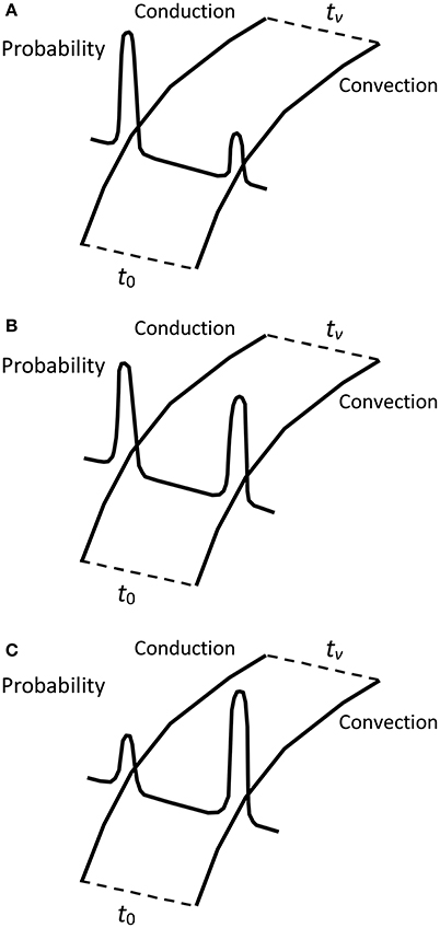
Figure 3. The Bénard experiment for temperature gradient (A) below the point of bifurcation, (B) at the point of bifurcation, (C) above the point of bifurcation.

We have considered near equilibrium processes and stationary dissipative structures. But non-equilibrium processes are in no way limited to these two extremes. We may consider a significantly non-equilibrium process when even the local equilibrium is not reached and we do not have temperature or pressure defined even locally. The formalism developed in our study remains applicable for this general case as well, leading to the description of non-equilibrium phase transitions even for such complex processes far from equilibrium.

In statistical physics, many questions about the path integral approach are still opened. And damage phenomena are probably a crucial step for these studies due to the intrinsic property of damage growth as being a non-equilibrium process. Besides, damage evolution is often more illustrative than thermodynamical models of statistical physics can provide. We hope that the application of non-equilibrium statistical physics to damage phenomena will be beneficial for the further development of statistical physics itself as it has already taken place, for example, with complex systems.

Author Contributions

The author confirms being the sole contributor of this work and approved it for publication.

Conflict of Interest Statement

The author declares that the research was conducted in the absence of any commercial or financial relationships that could be construed as a potential conflict of interest.

References

1. Barenblatt GI, Botvina LR. Self-similarity of fatigue failure. Damage accumulation. Izv AN SSSR MTT. (1983) 4:161–5.

2. Smalley RF, Turcotte DL, Solla SA. A renormalization group approach to the stick-slip behavior of faults. J Geophys Res Solid Earth Planets (1985) 90:1894–900.

Google Scholar

3. Rundle JB, Klein W. Nonclassical nucleation and growth of cohesive tensile cracks. Phys Rev Lett. (1989) 63:171–4.

PubMed Abstract | Google Scholar

4. Sornette A, Sornette D. Earthquake rupture as a critical-point: consequences for telluric precursors. Tectonophysics (1990) 179:327–34.

Google Scholar

5. Blumberg Selinger RL, Wang ZG, Gelbart WM, Ben-Shaul A. Statistical-thermodynamic approach to fracture. Phys Rev A (1991) 43:4396–400.

Google Scholar

6. Sornette D, Sammis CG. Complex critical exponents from renormalization-group theory of earthquakes: implications for earthquake predictions. J Phys I (1995) 5:607–19.

Google Scholar

7. Buchel A, Sethna JP. Elastic theory has zero radius of convergence. Phys Rev Lett. (1996) 77:1520–23.

PubMed Abstract | Google Scholar

8. Andersen JV, Sornette D, Leung KT. Tricritical behavior in rupture induced by disorder. Phys Rev Lett. (1997) 78:2140–43.

Google Scholar

9. Buchel A, Sethna JP. Statistical mechanics of cracks: fluctuations, breakdown, and asymptotics of elastic theory. Phys Rev E (1997) 55:7669–90.

Google Scholar

10. Zapperi S, Ray P, Stanley HE, Vespignani A. First-order transition in the breakdown of disordered media. Phys Rev Lett. (1997) 78:1408–11.

Google Scholar

11. Sornette D, Andersen JV. Scaling with respect to disorder in time-to-failure. Eur Phys J B (1998) 1:353–7.

Google Scholar

12. Zapperi S, Ray P, Stanley HE, Vespignani A. Analysis of damage clusters in fracture processes. Phys A Stat Mech Appl. (1999) 270:57–62.

Google Scholar

13. Zapperi S, Ray P, Stanley HE, Vespignani A. Avalanches in breakdown and fracture processes. Phys Rev E (1999) 59:5049–57.

PubMed Abstract | Google Scholar

14. Krajcinovic D, van Mier J editors. Damage and fracture of disordered materials. In: CISM Courses and Lectures. Vienna: Springer (2000).

Google Scholar

15. Naimark OB, Davydova M, Plekhov OA, Uvarov SV. Nonlinear and structural aspects of transitions from damage to fracture in composites and structures. Comput Struct. (2000) 76:67–75. doi: 10.1016/S0045-7949(99)00175-3

CrossRef Full Text | Google Scholar

16. Pride SR, Toussaint R. Thermodynamics of fiber bundles. Phys A Stat Mech Appl. (2002) 312:159–71. doi: 10.1016/S0378-4371(02)00816-6

CrossRef Full Text | Google Scholar

17. Naimark OB. Defect-induced transitions as mechanisms of plasticity and failure in multifield continua. In: Capriz G, Mariano PM, editors. Advances in Multifield Theories for Continua with Substructure. Boston, MA: Birkhäuser (2004) 75–114.

Google Scholar

18. Sornette D, Ouillon G. Multifractal scaling of thermally activated rupture processes. Phys Rev Lett. (2005) 94:038501. doi: 10.1103/PhysRevLett.94.038501

PubMed Abstract | CrossRef Full Text | Google Scholar

19. Toussaint R, Pride SR. Interacting damage models mapped onto Ising and percolation models. Phys Rev E (2005) 71:046127. doi: 10.1103/PhysRevE.71.046127

PubMed Abstract | CrossRef Full Text | Google Scholar

20. Barenblatt GI. Scaling phenomena in fatigue and fracture. Int J Fract. (2006) 138:19–35. doi: 10.1007/s10704-006-0036-0

CrossRef Full Text | Google Scholar

21. Abaimov SG. Applicability and non-applicability of equilibrium statistical mechanics to non-thermal damage phenomena. J Stat Mech. (2008) 9:P09005. doi: 10.1088/1742-5468/2008/09/P09005

CrossRef Full Text | Google Scholar

22. Abaimov SG. Applicability and non-applicability of equilibrium statistical mechanics to non-thermal damage phenomena: II. Spinodal behavior. J Stat Mech. (2009) 3:P03039. doi: 10.1088/1742-5468/2009/03/p03039

CrossRef Full Text | Google Scholar

23. Abaimov SG, Cusumano JP. Nucleation phenomena in an annealed damage model: Statistics of times to failure. Phys Rev E (2014) 90:062401. doi: 10.1103/PhysRevE.90.062401

PubMed Abstract | CrossRef Full Text | Google Scholar

24. Abaimov SG, Akhatov IS. Non-thermal quenched damage phenomena: The application of the mean-field approach for the three-dimensional case. AIP Adv. (2016) 6:095116. doi: 10.1063/1.4963304

CrossRef Full Text | Google Scholar

25. Herrmann HJ, Roux S. Statistical Models for the Fracture of Disordered Media. Amsterdam: North-Holland (1990).

Google Scholar

26. Krajcinovic D. Damage Mechanics. Amsterdam: Elsevier (1996).

Google Scholar

27. Chakrabarti BK, Benguigui LG. Statistical Physics of Fracture and Breakdown in Disordered Systems. Oxford: Clarendon Press (1997).

Google Scholar

28. Bhattacharyya P, Chakrabarti BK, editors. Modelling Critical and Catastrophic Phenomena in Geoscience. Lecture Notes in Physics. Berlin: Springer (2006).

Google Scholar

29. Sornette D. Critical Phenomena in Natural Sciences. Berlin: Springer (2006).

Google Scholar

30. Abaimov SG. Statistical Physics of Non-thermal Phase Transitions: From Foundations to Applications. Cham; Heidelberg; New York, NY; Dordrecht; London: Springer (2015).

Google Scholar

31. Kun F, Zapperi S, Herrmann HJ. Damage in fiber bundle models. Eur Phys J B (2000) 17:269–79. doi: 10.1007/PL00011084

CrossRef Full Text | Google Scholar

32. Moreno Y, Gómez JB, Pacheco AF. Fracture and second-order phase transitions. Phys Rev Lett. (2000) 85:2865–8. doi: 10.1103/PhysRevLett.85.2865

PubMed Abstract | CrossRef Full Text | Google Scholar

33. Moreno Y, Gómez JB, Pacheco AF. Phase transitions in load transfer models of fracture. Phys A Stat Mech Appl. (2001) 296:9–23. doi: 10.1016/S0378-4371(01)00018-8

CrossRef Full Text | Google Scholar

34. Pradhan S, Bhattacharyya P, Chakrabarti BK. Dynamic critical behavior of failure and plastic deformation in the random fiber bundle model. Phys Rev E (2002) 66:016116. doi: 10.1103/PhysRevE.66.016116

PubMed Abstract | CrossRef Full Text | Google Scholar

35. Bhattacharyya P, Pradhan S, Chakrabarti BK. Phase transition in fiber bundel models with recursive dynamics. Phys Rev E (2003) 67:046122. doi: 10.1103/PhysRevE.67.046122

PubMed Abstract | CrossRef Full Text | Google Scholar

36. Pierce FT. Tensile tests for cotton yarns: V. The “weakest link” theorems on the strength of long and of composite specimens. J Textile Inst Trans. (1926) 17:T355–68.

37. Daniels HE. The statistical theory of the strength of bundles of threads. I. Proc R Soc A (1945) 183:405–35.

Google Scholar

38. Coleman BD. On the strength of classical fibres and fibre bundles. J Mech Phys Solids (1958) 7:60–70.

Google Scholar

39. Suh MW, Bhattacharyya BB, and Grandage A. On the distribution and moments of the strength of a bundle of filaments. J Appl Probabil. (1970) 7:712–20.

Google Scholar

40. Phoenix S L, Taylor HM. The asymptotic strength distribution of a general fiber bundle. Adv Appl Probabil. (1973) 5:200–16.

Google Scholar

41. Sen PK. An asymptotically efficient test for the bundle strength of filaments. J Appl Probabil. (1973) 10:586–96.

Google Scholar

42. Sen PK. On fixed size confidence bands for the bundle strength of filaments. Ann Stat. (1973) 1:526–37.

Google Scholar

43. Harlow DG, Phoenix SL. The chain-of-bundles probability model for the strength of fibrous materials I: analysis and conjectures. J Comp Mater. (1978) 12:195–214.

Google Scholar

44. Phoenix SL. Statistical aspects of failure of fibrous materials. In: Tsai SW, editor Composite Materials: Testing and Design. Philadelphia, PA: ASTM (1979) 455–483.

Google Scholar

45. Smith RL. A probability model for fibrous composites with local load sharing. Proc R Soc A (1980) 372:539–53.

Google Scholar

46. Harlow DG, Phoenix SL. Probability distributions for the strength of composite materials I: Two-level bounds. Int J Fract. (1981) 17:347–72. doi: 10.1007/BF00036188

CrossRef Full Text | Google Scholar

47. Harlow DG, Phoenix SL. Probability distributions for the strength of composite materials II: a convergent sequence of tight bounds. Int J Fract. (1981) 17:601–30.

Google Scholar

48. Smith RL, Phoenix SL. Asymptotic distributions for the failure of fibrous materials under series-parallel structure and equal load-sharing. J Appl Mech. (1981) 48:75–82.

Google Scholar

49. Harlow DG, Phoenix SL. Probability distributions for the strength of fibrous materials under local load sharing. I. Two-level failure and edge effects. Adv Appl Probabil. (1982) 14:68–94.

Google Scholar

50. Krajcinovic D, Silva MAG. Statistical aspects of the continuous damage theory. Int J Solids Struct. (1982) 18:551–62.

Google Scholar

51. Smith RL. The asymptotic distribution of the strength of a series-parallel system with equal load-sharing. Ann Probabil. (1982) 10:137–71.

Google Scholar

52. Phoenix SL, Smith RL. A comparison of probabilistic techniques for the strength of fibrous materials under local load-sharing among fibers. Int J Solids Struct. (1983) 19:479–96.

Google Scholar

53. Daniels HE, Skyrme THR. The maximum of a random walk whose mean path has a maximum. Adv Appl Probabil. (1985) 17:85–99.

Google Scholar

54. Harlow DG. The pure flaw model for chopped fibre composites. Proc R Soc A (1985) 397:211–32.

Google Scholar

55. Daniels HE. The maximum of a Gaussian process whose mean path has a maximum, with an application to the strength of bundles of fibres. Adv Appl Probabil. (1989) 21:315–33.

Google Scholar

56. Sornette D. Elasticity and failure of a set of elements loaded in parallel. J Phys A (1989) 22:L243–50.

Google Scholar

57. Sornette D, Redner S. Rupture in the bubble model. J Phys A (1989) 22:L619–25.

Google Scholar

58. Harlow DG, Phoenix SL. Approximations for the strength distribution and size effect in an idealized lattice model of material breakdown. J Mech Phys Solids (1991) 39:173–200.

Google Scholar

59. Hemmer PC, Hansen A. The distribution of simultaneous fiber failures in fiber bundles. J Appl Mech. (1992) 59:909–14.

Google Scholar

60. Phoenix SL, Raj R. Scalings in fracture probabilities for a brittle matrix fiber composite. Acta Metal Mater. (1992) 40:2813–28.

Google Scholar

61. Sornette D. Mean-field solution of a block-spring model of earthquakes. J Phys I (1992) 2:2089–96.

Google Scholar

62. Gómez JB, Iñiguez D, Pacheco AF. Solvable fracture model with local load transfer. Phys Rev Lett. (1993) 71:380–83.

PubMed Abstract | Google Scholar

63. Krajcinovic D, Lubarda V, Sumarac D. Fundamental aspects of brittle cooperative phenomena - effective continua models. Mech Mater. (1993) 15:99–115.

Google Scholar

64. Duxbury PM, Leath PL. Exactly solvable models of material breakdown. Phys Rev B (1994) 49:12676–87.

PubMed Abstract | Google Scholar

65. Hansen A, Hemmer PC. Burst avalanches in bundles of fibers: local versus global load-sharing. Phys Lett A (1994) 184:394–6.

Google Scholar

66. Hansen A, Hemmer PC. Criticality in fracture: the burst distribution. Trends Stat Phys.(1994) 1:213–24.

67. Leath PL, Duxbury PM. Fracture of heterogeneous materials with continuous distributions of local breaking strengths. Phys Rev B (1994) 49:14905.

PubMed Abstract | Google Scholar

68. Lee W. Burst process of stretched fiber bundles. Phys Rev E (1994) 50:3797.

PubMed Abstract | Google Scholar

69. Sornette D. Sweeping of an instability: an alternative to self-organized criticality to get powerlaws without parameter tuning. J Phys I (1994) 4:209–21.

Google Scholar

70. Zhang SD, Ding EJ. Burst-size distribution in fiber-bundles with local load-sharing. Phys Lett A (1994) 193:425–30.

Google Scholar

71. Zhang, SD, Ding EJ. Failure of fiber bundles with local load sharing. Phys Rev B (1996) 53:646–54.

PubMed Abstract | Google Scholar

72. Kloster M, Hansen A, Hemmer PC. Burst avalanches in solvable models of fibrous materials. Phys Rev E (1997) 56:2615–25.

Google Scholar

73. Curtin WA, Takeda N. Tensile strength of fiber-reinforced composites: I. Model and effects of local fiber geometry. J Comp Mater. (1998) 32:2042–59.

Google Scholar

74. da Silveira R. Comment on ‘Tricritical behavior in rupture induced by disorder’. Phys Rev Lett. (1998) 80:3157.

Google Scholar

75. Delaplace A, Roux S, Pijaudier-Cabot G. Damage cascade in a softening interface. Int J Solids Struct. (1999) 36:1403–26.

Google Scholar

76. Roux S, Delaplace A, Pijaudier-Cabot G. Damage at heterogeneous interfaces. Phys A Stat Mech Appl (1999) 270:35–41.

Google Scholar

77. da Silveira R. An introduction to breakdown phenomena in disordered systems. Am J Phys. (1999) 67:1177–88.

Google Scholar

78. Moreno Y, Gómez JB, Pacheco AF. Self-organized criticality in a fibre-bundle-type model. Phys A Stat Mech Appl. (1999) 274:400–9.

Google Scholar

79. Wu BQ, Leath PL. Failure probabilities and tough-brittle crossover of heterogeneous materials with continuous disorder. Phys Rev B (1999) 59:4002. doi: 10.1103/PhysRevB.59.4002

CrossRef Full Text | Google Scholar

80. Hidalgo RC, Kun F, Herrmann HJ. Bursts in a fiber bundle model with continuous damage. Physical Review E (Statistical, Nonlinear, and Soft Matter Physics), 64(6), 066122 (2001)

PubMed Abstract | Google Scholar

81. Batrouni GG, Hansen A, Schmittbuhl J. Heterogeneous interfacial failure between two elastic blocks. Phys Rev E Stat Nonlin Soft Matter Phys. (2002) 65:036126. doi: 10.1103/PhysRevE.65.036126

PubMed Abstract | CrossRef Full Text | Google Scholar

82. Hidalgo RC, Moreno Y, Kun F, Herrmann HJ. Fracture model with variable range of interaction. Phys Rev E Stat Nonlin Soft Matter Phys. (2002) 65:046148. doi: 10.1103/PhysRevE.65.046148

PubMed Abstract | CrossRef Full Text | Google Scholar

83. Pradhan S, Hansen A, Chakrabarti BK. Failure processes in elastic fiber bundles. (2008) arXiv:0808.1375.

Google Scholar

84. Pradhan S, Hansen A, Chakrabarti BK. Failure processes in elastic fiber bundles. Rev Modern Phys. (2010) 82:499. doi: 10.1103/RevModPhys.82.499

CrossRef Full Text | Google Scholar

85. Hansen A, Hemmer P, Pradhan S. The Fiber Bundle Model. Weinheim: Wiley-VCH. (2015).

Google Scholar

86. Coleman BD. Time dependence of mechanical breakdown phenomena. J Appl Phys. (1956) 27:862–6. doi: 10.1063/1.1722504

CrossRef Full Text | Google Scholar

87. Coleman BD. Time dependence of mechanical breakdown in bundles of fibers. I. Constant total load. J Appl Phys. (1957) 28:1058–64. doi: 10.1063/1.1722907

CrossRef Full Text | Google Scholar

88. Coleman BD, Marquardt DW. Time dependence of mechanical breakdown in bundles of fibers. II. The infinite ideal bundle under linearly increasing loads. J Appl Phys. (1957) 28:1065–7.

Google Scholar

89. Birnbaum ZW, Saunders SC. A statistical model for life-length of materials. J Am Stat Assoc. (1958) 53:151–9.

Google Scholar

90. Coleman BD. Statistics and time dependence of mechanical breakdown in fibers. J Appl Phys. (1958) 29:968–83.

Google Scholar

91. Coleman BD. Time dependence of mechanical breakdown in bundles of fibers. III. The power law breakdown rule. Trans Soc Rheol (1958) 2:195–218.

Google Scholar

92. Coleman BD. Time dependence of mechanical breakdown in bundles of fibers. IV. Infinite ideal bundle under oscillating loads. J Appl Phys. (1958) 29:1091–9.

Google Scholar

93. Phoenix SL. The asymptotic time to failure of a mechanical system of parallel members. SIAM J Appl Math. (1978) 34:227–46.

Google Scholar

94. Phoenix SL. Stochastic strength and fatigue of fiber bundles. Int J Fract. (1978) 14:327–44.

Google Scholar

95. Phoenix SL. The asymptotic distribution for the time to failure of a fiber bundle. Adv Appl Probabil. (1979) 11:153–87.

Google Scholar

96. Phoenix SL, Tierney LJ. A statistical model for the time dependent failure of unidirectional composite materials under local elastic load-sharing among fibers. Eng Fract Mech. (1983) 18:193–215.

Google Scholar

97. Gómez JB, Moreno Y, Pacheco AF. Probabilistic approach to time-dependent load-transfer models of fracture. Phys Rev E Stat Nonlin Soft Matter Phys. (1998) 58:1528–32.

Google Scholar

98. Vázquez-Prada M, Gómez JB, Moreno Y, Pacheco AF. Time to failure of hierarchical load-transfer models of fracture. Phys Rev E Stat Nonlin Soft Matter Phys. (1999) 60:2581–94.

PubMed Abstract | Google Scholar

99. Zhang SD. Scaling in the time-dependent failure of a fiber bundle with local load sharing. Phys Rev E Stat Nonlin Soft Matter Phys. (1999) 59:1589–92.

Google Scholar

100. Moral L, Gómez JB, Moreno Y, Pacheco AF. Exact numerical solution for a time-dependent fibre-bundle model with continuous damage. J Phys A (2001) 34:9983–91. doi: 10.1088/0305-4470/34/47/305

CrossRef Full Text | Google Scholar

101. Moral L, Moreno Y, Gómez JB, Pacheco AF. Time dependence of breakdown in a global fiber-bundle model with continuous damage. Phys Rev E Stat Nonlin Soft Matter Phys. (2001) 63:066106. doi: 10.1103/PhysRevE.63.066106

PubMed Abstract | CrossRef Full Text | Google Scholar

102. Moreno Y, Correig AM, Gómez JB, Pacheco AF. A model for complex aftershock sequences. J Geophys Res Solid Earth (2001) 106:6609–19. doi: 10.1029/2000JB900396

CrossRef Full Text | Google Scholar

103. Newman WI, Phoenix SL. Time-dependent fiber bundles with local load sharing. Phys Rev E (2001) 63:021507. doi: 10.1103/PhysRevE.63.021507

PubMed Abstract | CrossRef Full Text | Google Scholar

104. Turcotte DL, Newman WI, Shcherbakov R. Micro and macroscopic models of rock fracture. Geophys J Int. (2003) 152:718–28. doi: 10.1046/j.1365-246X.2003.01884.x

CrossRef Full Text | Google Scholar

105. Yewande OE, Moreno Y, Kun F, Hidalgo RC, Herrmann HJ. Time evolution of damage under variable ranges of load transfer. Phys Rev E (2003) 68:026116. doi: 10.1103/PhysRevE.68.026116

PubMed Abstract | CrossRef Full Text | Google Scholar

106. Turcotte DL, Glasscoe, MT. A damage model for the continuum rheology of the upper continental crust. Tectonophysics (2004) 383:71–80. doi: 10.1016/j.tecto.2004.02.011

CrossRef Full Text | Google Scholar

107. Nanjo KZ, Turcotte DL. Damage and rheology in a fibre-bundle model. Geophys J Int. (2005) 162:859–66. doi: 10.1111/j.1365-246X.2005.02683.x

CrossRef Full Text | Google Scholar

108. Sornette D, Andersen, JV. Optimal prediction of time-to-failure from information revealed by damage. Europhys Lett. (2006) 74:778–84. doi: 10.1209/epl/i2006-10036-6

CrossRef Full Text | Google Scholar

109. Phoenix SL, Newman WI. Time-dependent fiber bundles with local load sharing. II. General Weibull fibers. Phys Rev E (2009) 80:066115. doi: 10.1103/PhysRevE.80.066115

PubMed Abstract | CrossRef Full Text | Google Scholar

110. Sornette D, Vanneste C. Dynamics and memory effects in rupture of thermal fuse networks. Phys Rev Lett. (1992) 68:612–15. doi: 10.1103/PhysRevLett.68.612

PubMed Abstract | CrossRef Full Text | Google Scholar

111. Sornette D, Vanneste C, Knopoff L. Statistical model of earthquake foreshocks. Phys Rev A (1992) 45:8351–7. doi: 10.1103/PhysRevA.45.8351

PubMed Abstract | CrossRef Full Text | Google Scholar

112. Vanneste C, Sornette D. The dynamical thermal fuse model. J Phys I (1992) 2:1621–44. doi: 10.1051/jp1:1992231

CrossRef Full Text | Google Scholar

113. Guarino A, Scorretti R, Ciliberto S. Material failure time and the fiber bundle model with thermal noise. (1999) arXiv, cond-mat/9908329v1, 1–11.

Google Scholar

114. Roux S. Thermally activated breakdown in the fiber-bundle model. Phys Rev E (2000) 62:6164–9. doi: 10.1103/PhysRevE.62.6164

PubMed Abstract | CrossRef Full Text | Google Scholar

115. Ciliberto S, Guarino A, Scorretti R. The effect of disorder on the fracture nucleation process. Phys D (2001) 158:83–104. doi: 10.1016/S0167-2789(01)00306-2

CrossRef Full Text | Google Scholar

116. Scorretti R, Ciliberto S, Guarino A. Disorder enhances the effects of thermal noise in the fiber bundle model. Europhys Lett. (2001) 55:626–32. doi: 10.1209/epl/i2001-00462-x

CrossRef Full Text | Google Scholar

117. Politi A, Ciliberto S, Scorretti R. Failure time in the fiber-bundle model with thermal noise and disorder. Phys Rev E (2002) 66:026107. doi: 10.1103/PhysRevE.66.026107

PubMed Abstract | CrossRef Full Text | Google Scholar

118. Saichev A, Sornette D. Andrade, Omori, and time-to-failure laws from thermal noise in material rupture. Phys Rev E (2005) 71:016608. doi: 10.1103/PhysRevE.71.016608

PubMed Abstract | CrossRef Full Text | Google Scholar

119. Pauchard L, Meunier J. Instantaneous and time-lag breaking of a two-dimensional solid rod under a bending stress. Phys Rev Lett. (1993) 70:3565–8. doi: 10.1103/PhysRevLett.70.3565

PubMed Abstract | CrossRef Full Text | Google Scholar

120. Bonn D, Kellay H, Prochnow M, Ben-Djemiaa K, Meunier J. Delayed fracture of an inhomogeneous soft solid. Science (1998) 280:265–7. doi: 10.1126/science.280.5361.265

PubMed Abstract | CrossRef Full Text | Google Scholar

121. Sollich P. Rheological constitutive equation for a model of soft glassy materials. Physical Rev E (1998) 58:738–59. doi: 10.1103/PhysRevE.58.738

CrossRef Full Text | Google Scholar

122. Guarino A, Ciliberto S, Garcimartín A. Failure time and microcrack nucleation. Europhys Lett. (1999) 47:456–61. doi: 10.1209/epl/i1999-00409-9

CrossRef Full Text | Google Scholar

123. Guarino A, Ciliberto S, Garcimartín A, Zei M, Scorretti R. Failure time and critical behaviour of fracture precursors in heterogeneous materials. Eur Phys J B (2002) 26:141–51. doi: 10.1140/epjb/e20020075

CrossRef Full Text | Google Scholar

124. Arndt PF, Nattermann T. Criterion for crack formation in disordered materials. Phys Rev B (2001) 63:134204. doi: 10.1103/PhysRevB.63.134204

CrossRef Full Text | Google Scholar

125. Abaimov SG. Non-equilibrium statistical mechanics of non-equilibrium damage phenomena. (2009) arXiv, 0905.0292.

Google Scholar

126. Abaimov SG. General formalism of non-equilibrium statistical mechanics, a path approach. (2009) arXiv, 0906.0190.

Google Scholar

127. Leontovich MA. On the free energy of the nonequilibrium state. ZhETF (1938) 8:844–54.

128. Leontovich MA. Introduction to Thermodynamics. Statistical Physics. Moscow: Nauka (1983).

129. Grandy WT. Entropy and the Time Evolution of Macroscopic Systems. Oxford: Oxford University Press (2008).

130. Grandy WT. Foundations of Statistical Mechanics. Dordrecht: D. Reidel Publishing Company (1988).

Google Scholar

131. Onsager L, Machlup S. Fluctuations and irreversible processes. Phys Rev. (1953) 91:1505–12 doi: 10.1103/PhysRev.91.1505

CrossRef Full Text | Google Scholar

132. Kikuchi R. Irreversible cooperative phenomena. Ann Phys. (1960) 10:127–51. doi: 10.1016/0003-4916(60)90019-1

CrossRef Full Text | Google Scholar

133. Kikuchi R. Variational derivation of the steady state. Phys Rev. (1961) 124:1682–91. doi: 10.1103/PhysRev.124.1682

CrossRef Full Text | Google Scholar

134. Lavenda BH, Cardella C. On the persistence of irreversible processes under the influence of random thermal fluctuations. J Phys Math A Gen. (1986) 19:395–407.

Google Scholar

135. Ishii T. The path probability ansatz and master equation. Prog Theor Phys Suppl. (1994) 115:243–54. doi: 10.1143/PTPS.115.243

CrossRef Full Text | Google Scholar

136. Dewar R. Information theory explanation of the fluctuation theorem, maximum entropy production and self-organized criticality in non-equilibrium stationary states. J Phys A Math Gen. (2003) 36:631–41. doi: 10.1088/0305-4470/36/3/303

CrossRef Full Text | Google Scholar

137. Woo HJ. Statistics of nonequilibrium trajectories and pattern selection. Europhys Lett. (2003) 64:627–33. doi: 10.1209/epl/i2003-00274-6

CrossRef Full Text | Google Scholar

138. Evans RML. Driven steady states: rules for transition rates. Phys A Stat Mech Appl. (2004) 340:364–72. doi: 10.1016/j.physa.2004.04.028

CrossRef Full Text | Google Scholar

139. Evans RML. Rules for transition rates in nonequilibrium steady states. Phys Rev Lett. (2004) 92:150601. doi: 10.1103/PhysRevLett.92.150601

PubMed Abstract | CrossRef Full Text | Google Scholar

140. Evans RML. Detailed balance has a counterpart in non-equilibrium steady states. J Phys A Math Gen. (2005) 38:293–313. doi: 10.1088/0305-4470/38/2/001

CrossRef Full Text | Google Scholar

141. Lin TL, Wang R, Bi WP, El Kaabouchi A, Pujos C, Calvayrac F et al. Path probability distribution of stochastic motion of non dissipative systems: a classical analog of Feynman factor of path integral. Chaos Solitons Fractals (2013) 57:129–36. doi: 10.1016/j.chaos.2013.10.002

CrossRef Full Text | Google Scholar

142. Wang QA, El Kaabouchiu A. From random motion of hamiltonian systems to Boltzmann's H theorem and second law of thermodynamics: a pathway by path probability. Entropy (2014) 16:885–94. doi: 10.3390/e16020885

CrossRef Full Text | Google Scholar