A Hamiltonian Driven Quantum-Like Model for Overdistribution in Episodic Memory Recollection

1. Introduction - The Episodic Memory

In an early effort to systematize the developing science of memory, Tulving [5] aimed to provide operative definitions for presumed various categories of memory. Continuing a dichotomic approach, he proposed to complement the previously coined “semantic” memory with the “episodic” memory. While our “semantic” memory would allow us to regain facts and abstract knowledge about our world, our “episodic” memory would let us recall personally lived events in a specific spatio-temporal context from our past. While distinct, both were still considered partially overlapping information processing systems. With Mandler's [6] dual process approach it became more clear to distinguish the more contrived recollection by details with respect to the recall of facts [7]. In the dual recollection-familiarity process models a cue is processed respectively either in terms of remembering an event's details up to its genuine recollection, or by retrieving a feature which is associated to the cue so it becomes familiar and conflated with a truly episodic memory.

Jacoby [8] pointed out a confusion of the recollection-familiarity process with the retrieval task itself. He urged for explicit process dissociation providing two separate parameters for the aspects of recollection—or intentional memory use—and for familiarity—or automatic memory use—in the dual process. In a further developed dual process approach the “conjoint recognition” model of Brainerd et al. [9] proposes separate parameters for the processes of; identity judgment, similarity judgment, and response bias. The latter model is able to implement the “fuzzy trace” theory (FTT) with its identity vs. similarity distinction. Reyna and Brainerd [10] crucially distinguishes verbatim and gist dimensions to memories. Verbatim traces hold the detailed contextual features of a past event, while gist traces hold its semantic—“fuzzy”—details. Our brain would analyze a past event by accessing its stored verbatim and gist trace in parallel. On the one hand the verbatim trace of a verbal cue handles it “surface” content—i.e., orthography and phonology for words—with its contextual features, while the verbal cue's gist trace will encode “relational” content—i.e., semantic content for words—with its contextual features. In more recent work the FTT model has received a quantum probabilistic formalization to cope with overdistribution in memory tests [1, 4, 11, 12]. While we are essentially connecting to this line of research with our present quantum model, a wide variety of recollection memory models have been developed in the literature that are not discussed here. We do refer to one specific semantic network approach by Nelson et al. [13] and Bruza et al. [14] which also infers quantum structures for its development. In essence their model proposes a semantically associated network, in which a target word is adjacent to all associated terms according the natural language of its users. It has been shown best prediction of memory performance is obtained by implementing the network in a quantum superposition state of either complete activation—amplitude 1—or non-activation—amplitude 0. The model provides weighed directional word associations, and a quantumlike entanglement between nodes is invoked to predict parallel instead of serial activation of neighbors. We have not included the Nelson and McEvoy model in our present discussion since it has not been developed to explicitly implement a gist-verbatim distinction with respect to which the EOD effect we target here is developed.

The EOD effect. One striking phenomenon concerning memory is the Episodic Over-distribution effect—or EOD. More or less this effect expresses a person's proneness to conflate memories of distinct events. More precisely the effect points out we tend to affiliate “alien” memories to true memories concerning a given event, leading to an “exaggeration” of memories concerning that event.

In Brainerd et al. [3] the disjunction fallacy is modeled for the item false memory paradigm while the source false memory version is covered in Brainerd et al. [15]. Brainerd et al. [1] exposes the more common case of subadditivity of episodic memory.

These EOD effects are shown in specifically designed experiments: the item false memory experiment in 2015 is a modification (also 2, 3, 9) of a classical paradigm in which a single “instruction” (or probe) would be given to measure whether “a given cue is a target (or not).”

EOD–subadditivity. In the item false memory (IFM) experiment three possible cues “old”—or o, “new-similar”—or ns, and “new-dissimilar”—or nd are presented. These cues are crossed with three “probes” namely o?, ns?, and nd?. These probes “o?, ns?, and nd?,” respectively, enquire the participant “is this probe old?” (studied before), “is this probe new but similar?” (semantically related to the old cues but not literally among them) and “is this probe new and dissimilar?” (has nothing to do with with the studied cues, even not semantically). In this experimental paradigm after exposure to an unidentified cue the participant is enquired by one of three distinct probes.

In practice most of the IFM experiments turn out subadditive acceptance probabilities:

$\begin{array}{ll}p(o?)+p(ns?)+p(nd?)>1.& (1)\end{array}$

That is, the disjoint partial features are over recalled with respect to its encompassing event. Notice that even if the law of total probability would be satisfied Brainerd mentions the possible issue of compensations; a systematic change in remembering ns as such may compensate a reverse change to remember ns as o, restoring the classical addition to 1.

EOD–disjunction fallacy. In the 2010-version of the IFM experiment a disjunctive probe was presented to the participants instead of the nd? probe. This probe questioned whether the cue was either “old” or “new-similar,” leaving unnecessary the answer to the question which one of both types the cue really was. A comparison of acceptance probability under the disjunctive probe o or ns? and the summed acceptance probabilities under the separate probes o? and ns? revealed a subadditive relation

$\begin{array}{llll}p(o?)+p(ns?)& >& p(oorns?).& (2)\end{array}$

This relation amounts to a disjunction fallacy since both cue types are mutually exclusive categories. The EOD effect was further identified using the unpacking factor of [16]

$\begin{array}{ll}\frac{p(o?)+p(ns?)}{p(oorns?)}>1.& (3)\end{array}$

the excess value of the fraction above one gives a measure of the amplitude of the effect.

Explanations of EOD effects. A number of theoretical explanations have been provided to interpret this phenomenon:

The fuzzy trace theory was implemented in QEM—the Quantum Episodic Memory model—by Brainerd et al. [1, 11]. By processing the perception of the verbatim and gist memory trace as separate components of a state vector, QEM allows to encompass the non-classical EOD probability effects of episodic memory. This capacity, we will see in the next section, is essentially due to the ubiquity of the gist component and its implementation in the corresponding outcome projectors for acceptance. Another quantum-like modeling perspective has been proposed by Busemeyer and Bruza [4, Ch.6] which provides unitary transformation matrices based on Feynman path analysis and ordering of the gist/verbatim processing of cues, which we will discuss below. Finally a complementarity based quantum-like development was done by Denolf and Subadditivity [17], and Denolf and Lambert-Mogiliansky [18]. Bohr's complementarity provides the gist–verbatim features by implementing for each an alternative basis of the Hilbert space. Our Hamiltonian development follows more closely the outline of the QEM model for FTT.

We will at present not make comparisons to either Markovian models [4, 19, 20] but focus on the possibility of Hamiltonian-driven time propagation in QEM, and compare to the Feynman path model and the original QEM model itself.

Experimental paradigms. A number of experimental paradigms have been proposed to test the over-distribution effect and the episodic disjunction effect. In this paper we mainly refer to Brainerd et al. [1, 3] which build and expand on “item false memory” and “source false memory” experimental paradigms, but only the former IFM paradigm will be modeled here. We shortly describe both paradigms of 2010 and 2015 for the IFM case. As we have mentioned, each of these paradigms consist of two consecutive stages.

2010 experimental paradigm. In the first stage participants studied a set {o} of memory targets consisting of words from a list of the Deese–Roediger–McDermott paradigm (DRM). The presented DRM lists are abbreviated sequences of the original 15 semantically related words that all associate forward to one common word. That latter word does not appear in the list and is therefore known as the distractor [21, 22]. We will in our approach not include the issue of the preliminary orienting task based on qualifying adjectives as positive, neutral, or negative, which “increase the processing of semantic content during subsequent exposure to word lists” [3]. After this memorization stage either immediate testing ensues or a time delay of a week is inserted. Subsequently a cue is presented to the participant and finally an instruction to respond to the cue is given.

Three possible types of cue are used; a studied target from {o} consisting of a word from one of the 24 lists, a related non-target from set {ns} consisting of words on the list but not learned ({o} ∩ {ns} = ϕ) and finally a new-dissimilar non-target from set {nd} with words not related in any sense to the selected DRM lists ({nd} ∩ {ns} = ϕ = {nd} ∩ {o}).

These cues are crossed with one of three instructions per participant¹. Either; the first instruction o? (or old?) to accept only an exact target from {o} and otherwise reject, or the second instruction ns? (new-similar?) to accept only a related non-target from {ns} otherwise reject, or a third instruction. The third instruction is o or ns? (or old or new-similar?) to accept either an exact target from {o} or a related non-target from {ns} and otherwise reject.

2015 experimental paradigm. The alternative version of the IFM paradigm of Brainerd et al. [1] follows precisely the two stages of the 2010-version except for the final stage. First the participants studied cues c of memory target words (24 times 6 in total). Then a time delay is either inserted or not. in the test phase participants are first exposed to a cue which is either a studied target from o, a new-similar non-target ns, or a new-dissimilar non-target nd. Finally the participant is asked to respond to one of three probes querying to which category the cue belongs; that is o?, ns?, or nd?. In comparison to the 2010-paradigm the o or ns? probe has been replaced by the nd? probe.

About the source false memory paradigm. In source false memory experiments the experimental paradigm focuses on the origin of the cue. It probes the source recollection in memory of cues originating from either List 1 or List 2 and crossed with probes List1?, List2?, and nd?. We will only focus our present Hamiltonian based quantum model on the IFM setting, it is however very possible to adapt the model to SFM requirements as well.

Besides the QEM model, this specific paradigm has been alternatively modeled by Denolf and Lambert–Mogiliansky using Bohr's quantum approach to consider gist and verbatim traces as complementary properties, each trace represented by an alternative bases of the same Hilbert space [18].

Experimental data in 2010 and 2015 paradigms. Since Brainerd et al. [1] focuses on subadditivity with the probes o?, ns?, or nd?, there is no interest in o or ns? thus it is not measured nor reported. While vice versa [3] has a focus on the disjunction fallacy, which reports o?, ns?, and o or ns? but does no reporting of nd cue data. We therefore take the data of Brainerd et al. [9] from which a full 3 × 3 grid of data can be reconstructed using an intervention proposed by Busemeyer and Bruza [4, p. 171].

In sum we have no data set which shows the subadditivity and the disjunction effect at the same time. We will thus adapt the parameters of the Hamiltonian model to each data set separately (see Tables 1, 2). We adopt Busemeyer's solution to complete the data set in the paradigm for the EOD disjunction effect by supplementing the nd probe data in the set through their response bias measures b_T, b_R, and b_{T + R} ([9]–Table 6). Moreover, we will fit to the average values over six experimental conditions here². While for the EOD subadditivity effect we will use ([1], Table 3, p. 233) in which we take the values for ns cue as the averages of ns-critical and ns-related cues, distinguished by Brainerd et al. [1].

TABLE 1

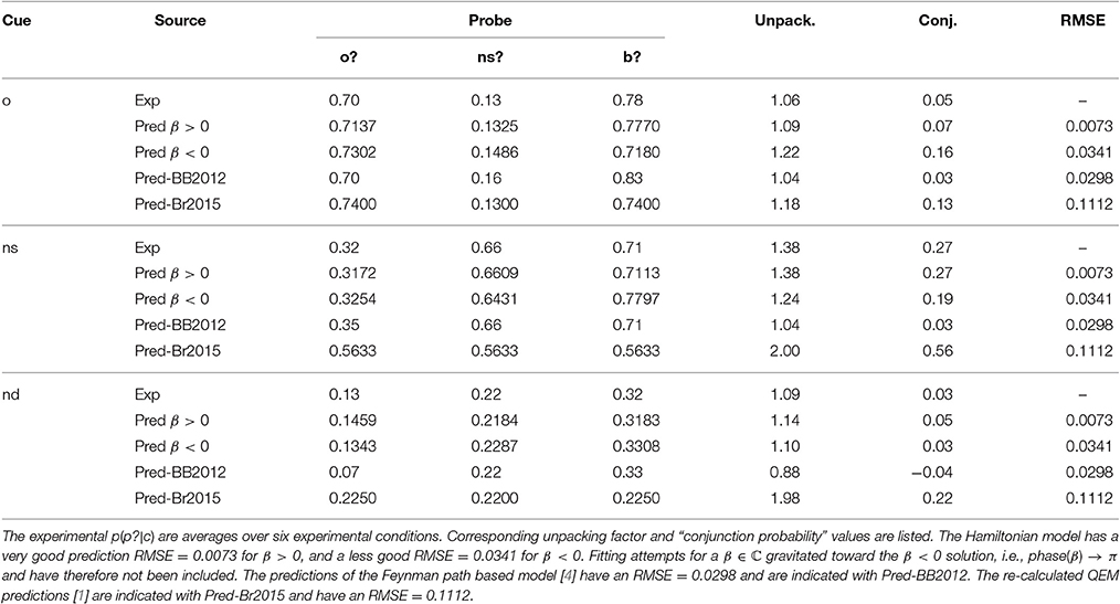
Table 1. EOD-disjunction fallacy: Experimental and predicted acceptance probabilities by probe and cue in item false memory paradigm - immediate test [9].

TABLE 2

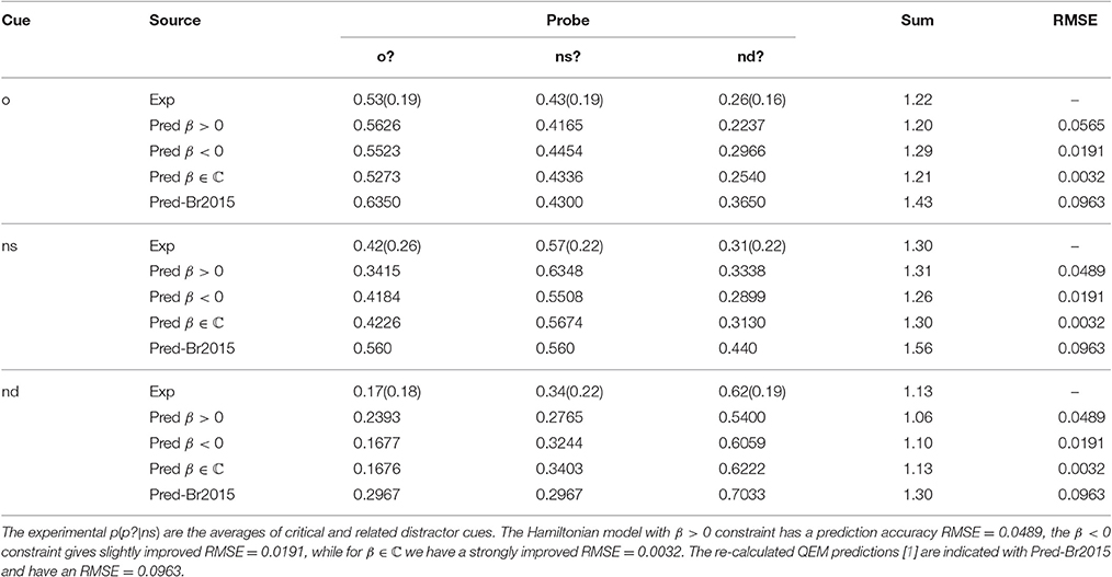
Table 2. EOD-subadditivity: Experimental and predicted acceptance probabilities by probe and cue in item false memory paradigm—immediate test [1].

2. Quantum Models

Probabilistic anomalies with respect to classical probability law have in many cases been successfully covered by models using quantum formalism, likewise the anomalies of EOD have been modeled in quantum-like manner. We shortly present some of these developments, mainly focussing on QEM.

2.1. The QEM Model by Brainerd et al.

Memory state vectors. QEM provides three orthogonal vectors in Hilbert space, respectively one for (verbal) surface form, one for semantical relatedness, and one for the case when neither of both previous are relatedly present. In line with the FTT these respective dimensions acquire probability amplitudes that represent the participant's mental state on the cue in the experiment, which we order as ${(v_c,g_c,n_c)}^{\tau }$³. The fact that these features are expressed by orthogonal vectors, reflects that these are perceived distinct properties of a word in memory. This orthogonality property should be differentiated from associative relationships of words like e.g., for a target word in a semantic memory network [13], which dominantly hinges on related gist but mostly leaves out related verbatim features. Brainerd et al. [1] and Brainerd and Reyna [2] describe the “perceived memory state” spanned by vectors in three-dimensional Hilbert space corresponding to verbatim, gist, and non-matching dimensions of the respective fuzzy traces for the set of words in the experimental paradigm in the brain:

$\begin{array}{ll}|S_c\rangle =v_c|V\rangle +g_c|G\rangle +n_c|N\rangle & (4)\end{array}$

Where c can be any cue type, o, ns, or nd, and each basis vector corresponds to respectively the fuzzy trace of form (V), semantic relation (G), and complete unrelatedness (N)⁴. According the model requirements—exhaustiveness and exclusiveness of the cues—the respective probabilities add up to unity

$\begin{array}{ll}|v_c{|}^2+|g_c{|}^2+|n_c{|}^2=1.& (5)\end{array}$

With these three normalizations constraints QEM requires the parameters {v_o, g_o, n_o, v_ns, g_ns, n_ns, v_nd, g_nd, n_nd} of which six are independent. We discuss some related fitting issues in QEM at the end of Section (2).

Acceptance projectors. A probe o?, ns?, or nd? is affirmatively—“yes” (y)—answered by applying the corresponding projection operator

$\begin{array}{ll}{M}_{y,o?}=\left[\begin{array}{ccc}1& 0& 0\\ 0& 1& 0\\ 0& 0& 0\end{array}\right],M_{y,ns?}=\left[\begin{array}{ccc}0& 0& 0\\ 0& 1& 0\\ 0& 0& 0\end{array}\right],M_{y,nd?}=\left[\begin{array}{ccc}0& 0& 0\\ 0& 0& 0\\ 0& 0& 1\end{array}\right]& (6)\end{array}$

on the state |S_c〉. These respective projector matrices are simply obtained by considering the final outcome vectors which they need to produce. In VGN space the projector M_y,nd? should lead to a vector proportional to (0, 0, 1), representing perception of no related verbatim nor gist of the nd cue. The form of this expected outcome vector (0, 0, 1) is directly related to the projector expression Equation (6, c). Similarly the projector M_y,ns?, Equation (6, b), is constructed from the expected outcome vector (0, 1, 0) representing only perception of related gist in the ns cue. For the projector matrix M_y,o? the outcome should lead into the space spanned by both related verbatim and gist components for the perception of the o cue. The latter is a two dimensional space spanned by the basis vectors (1, 0, 0) and (0, 1, 0), and is the outcome space of projector Equation (6, a). The β-parameter—present in the vector |o〉 for old cues—will allow to navigate such vectors in this two-dimensional subspace, altering the relative weight of the verbatim to gist components (see functioning of β in the description of the initial state, below).

In the experimental paradigm for the EOD disjunction fallacy the operator M_y,b? for the probe o or ns ? is used;

$\begin{array}{l}{M}_{y,b?}=M_{y,o?}+M_{y,ns?}-M_{y,o?}{M}_{y,ns?}\\ =M_{y,o?}& (7)\end{array}$

since M_y,o?M_y,ns? = M_y,ns?. In QEM the memory state for the experimental paradigm is posited to be |S_c〉 following the exposure to cue c. After providing the probe p the state collapses to the eigenvector of the projection operators M_y,p: “the cue elicits the memory state, and the probe determines the projector used to answer [affirmatively to] the question.” (1, p. 243).

The origin of EOD in QEM. Notice that the form of the projectors M_y,o? and M_y,ns? show that subadditivity is an immediate consequence of measuring the presence of the common gist trace in both operations. Which also implies—as Brainerd points out—the cases in which a gist trace would be lacking will not produce subadditivity. Similarly, we could remark that in the dual trace approach ns? is a subspace of o?. Therefore, the operator for the disjunctive probe coincides with the operator for the o? probe. As a consequence the EOD disjunction fallacy is not due to an interference dynamics in the QEM model, but follows from “double counting” the gist component in the outcome of disjunctive probe. Also the EOD subadditivity is due to this same double counting of gist. Both subadditivity and the disjunction fallacy are therefore considered “parameter-free” features of the QEM model [1]. In Section 2.3, we will cover the origin of the EOD effect more extensively and show how in our Hamiltonian approach of QEM one is not restricted to subadditive nor fallacious disjunctive scenarios.

The initial state. A short discussion on the initial state vector in the QEM model is needed since it plays an important role, both in Brainerd et al.'s development of QEM and our Hamiltonian driven version of the model. At the start of the experiment the participants of the experiment are informed about the equal probability by which each type of cue o, ns, or nd, will be presented [1].

It can be easily seen however that this is not possible to implement exactly without forcing this initial perceived memory state to be voided of all of its verbatim trace⁵. We claim a more appropriate representation of this initial state is done by addressing this uncertitude on the level of the probability amplitudes, not the probabilities themselves. More specifically, we implement each component probability amplitude is attributed equal weight $1/\sqrt{{N}}$ in the initial state

$\begin{array}{ll}|{\psi }_0\rangle =\frac{1}{\sqrt{\mathcal{N}}}\left(|o\rangle +|ns\rangle +|nd\rangle \right),\text{with}\Vert |{\psi }_0\rangle \Vert =1.& (8)\end{array}$

where ${N}$ is the vector's normalization factor. This initial state can be expressed in terms of perceived verbatim, gist, and unrelated components. The o-state is composed of components of verbatim and gist in the perceived memory according a superposition of both; |o〉 = α|V〉+β|G〉 or explicitly normalized ${(\sqrt{1-|\beta {|}^2},\beta ,0)}^{\tau }$, where β ∈ ℂ⁶. Thus both aspects V and G contribute with a variable amplitude to the targeted cue o—which a priori should have been expected since the relative magnitude of both traces seem variably dependent on the particular instance of the o-type cue. The memory states for ns and nd on the other hand do not decompose over multiple traces, and coincide with the unambiguous eigenvectors of the respective operators M_y,ns? and M_y,nd?, i.e., |ns〉 = |G〉 and |nd〉 = |N〉. The initial state prior to cue and probe presentation can thus be expressed in terms of orthogonal states for V, G, and N⁷:

$\begin{array}{ll}|{\psi }_0\rangle =\frac{1}{\sqrt{\mathcal{N}}}\left(\alpha |V\rangle +(1+\beta )|G\rangle +|N\rangle \right),\text{with}|\alpha {|}^2+|\beta {|}^2=1& (9)\end{array}$

from which we find an expression of the normalization factor

$\begin{array}{l}{N}=\sqrt{|\alpha {|}^2+|1+\beta {|}^2+1}=\sqrt{3+2\Re (\beta )}\end{array}$

of the initial state. Most importantly, we have a variable β in our description, which stands for the average amplitude of gist trace in the true target set {o} of the experimental paradigm. We assume that o cues with little relevance to the participants will correspond to low β, while o cues common to the participants will increase β.

Given the participant is informed she will be exposed to an equal amount of o, ns, and nd cues, overall she will expect an excess of gist in comparison to verbatim or unrelated features. A “constructive interference” in 1 + β with β > 0 would be expected (when β ∈ ℝ). In the present experimental paradigm the cues are semantically forward related words (to its target word) of the DRM lists, therefore we would expect low or moderate associated gist traces here, certainly not really intense gist traces as for instance the Madeleine-cue provoked in Marcel Proust.

2.2. The Feynman Path Model for EOD by Busemeyer et al.

The Feynman path model by Busemeyer and Trueblood [23] and Busemeyer and Bruza [4, Ch. 6] introduces a four dimensional Hilbert space to encompass the two orderings of the types of process; verbatim before gist on o cues, and gist before verbatim on ns and nd cues. This model thus provides a cue dependent construction of the memory state.

As in the QEM model, the Feynman path approach does not concatenate reflection time periods. The exposure of the cue or the probe to the participant does not engender a unitary time evolution of the memory state. Notably this model provides cue-dependence of evolution by ordering verbatim and gist stages in the process of recollection and depends on interference of probability amplitudes to form the acceptance probability in the disjunctive b? probe. Busemeyer and Bruza [4] model requires only 6 parameters for a satisfactory prediction of the 9 data points of the disjunctive EOD paradigm. The predictions of the Feynman path based model by Busemeyer et al. have been included in the data (Table 1). A short comparative discussion of the model's prediction capacity is given at the end of Section 2.

We summarize the Feynman paths in this model and have adapted the notation of Busemeyer and Bruza [4, Ch. 6] to conform with the present context⁸. We inserted the question mark to distinguish a probe—o?—from a cue o. The negation of a probe is indicated by the tilde sign—e.g., õ?—and corresponds to the negation of the instruction “Is this not an o cue?” This allows to express the complementarity of the cases o? and õ? according:

$\begin{array}{ll}|o\rangle \langle o|+|\tilde{o}\rangle \langle \tilde{o}|=𝕀& (10)\end{array}$

For o cues, verbatim is treated before gist, which means first o? operates on the initial state |S_o〉 for o cues, then followed by the operation of ns?:

$\begin{array}{l}p(o?|o)=|\langle o|S_o\rangle {|}^2,\\ p(ns?|o)=|\langle ns|S_o\rangle {|}^2=|\langle ns|o\rangle \langle o|S_o\rangle +\langle ns|\tilde{o}\rangle \langle \tilde{o}|S_o\rangle {|}^2,\\ p(b?|o)=p(o?|o)+p(\tilde{o}?|o)p(ns?|\tilde{o})\\ =|\langle o|S_o\rangle {|}^2+|\langle \tilde{o}|S_o\rangle {|}^2|\langle ns|\tilde{o}\rangle {|}^2,\\ =1-|\langle \tilde{n}s|\tilde{o}\rangle {|}^2|\langle \tilde{o}|S_o\rangle {|}^2,\end{array}$

requiring two parameters; 〈ns|o〉 and 〈ns|õ〉.

For ns cues gist is treated before verbatim, then first ns? operates on the initial state |S_ns〉 for ns cues, followed by o?

$\begin{array}{l}p(o?|ns)=|\langle o|S_{ns}\rangle {|}^2=|\langle o|ns\rangle \langle ns|S_{ns}\rangle +\langle o|\widetilde{ns}\rangle \langle \widetilde{ns}|S_{ns}\rangle {|}^2,\\ p(ns?|ns)=|\langle ns|S_{ns}\rangle {|}^2,\\ p(b?|ns)=p(ns?|ns)+p(\widetilde{ns}?|ns)p(o?|\widetilde{ns})\\ =|\langle ns|S_{ns}\rangle {|}^2+|\langle \widetilde{ns}|S_{ns}\rangle {|}^2|\langle o|\widetilde{ns}\rangle {|}^2,\\ =1-|\langle õ|\widetilde{ns}\rangle {|}^2|\langle \widetilde{ns}|ns\rangle {|}^2,\end{array}$

requiring two more parameters $\langle o|\widetilde{ns}\rangle$ and 〈o|ns〉.

Also for nd cues gist is treated before verbatim

$\begin{array}{l}p(o?|nd)=|\langle o|S_{nd}\rangle {|}^2=|\langle o|ns\rangle \langle ns|S_{nd}\rangle +\langle o|\widetilde{ns}\rangle \langle \widetilde{ns}|S_{nd}\rangle {|}^2,\\ p(ns?|nd)=|\langle ns|S_{nd}\rangle {|}^2,\\ p(b?|nd)=p(ns?|nd)+p(\widetilde{ns}?|nd)p(o?|\widetilde{nd})\\ =|\langle ns|S_{nd}\rangle {|}^2+|\langle \widetilde{ns}|S_{nd}\rangle {|}^2|\langle o|\widetilde{nd}\rangle {|}^2,\\ =1-|\langle õ|\widetilde{nd}\rangle {|}^2|\langle \widetilde{ns}|S_{nd}\rangle {|}^2,\end{array}$

without new parameter requirements. The parameters appear as elements of unitary transformations and must satisfy unitarity. Leaving $\langle ns|o\rangle =\sqrt{1-|\langle ns|õ\rangle {|}^2}=\langle \widetilde{ns}|õ\rangle$ and $\langle \widetilde{ns}|o\rangle =-{\langle ns|õ\rangle }^{\star }$. The initial state is described in a four dimensional Hilbert space, in which the initial state depends on the presented cue:

$\begin{array}{l}|S\rangle =|o_o\rangle \langle o_o|S\rangle +|{\tilde{o}}_o\rangle \langle {\tilde{o}}_o|S\rangle +|o_{\tilde{o}}\rangle \langle o_{\tilde{o}}|S\rangle +|{\tilde{o}}_{\tilde{o}}\rangle \langle {\tilde{o}}_{\tilde{o}}|S\rangle ,\\ =|n{s}_o\rangle \langle n{s}_o|S\rangle +|\tilde{n}{s}_o\rangle \langle \tilde{n}{s}_o|S\rangle +|n{s}_{\tilde{o}}\rangle \langle n{s}_{\tilde{o}}|S\rangle +|\tilde{n}{s}_{\tilde{o}}\rangle \langle \tilde{n}{s}_{\tilde{o}}|S\rangle .\end{array}$

where the index represents the cue type. The first expression is applicable for target cues from {o}, thus |S_o〉 (where the index õ indicates either ns or nd). And the second expression for the initial state is applicable when the cue is not a target but comes from {ns}∪{nd}, thus for |S_ns〉 and |S_nd〉. Therefore, 〈o_õ|S_o〉 = 〈õ_o|S_o〉 = 0 and $\langle n{s}_o|S_{õ}\rangle =\langle {\widetilde{ns}}_o|S_{õ}\rangle =0$. A simplification of the formalism is obtained by chosing the phase φ of 〈ns|õ〉 and the phase θ of $\langle o|\widetilde{ns}\rangle$ equal to each other. This choice corresponds to a simplification of the dynamics in the subspaces of the 4-dimensional Hilbert space, in which the gist-before-verbatim states and the verbatim-before-gist states differ. Equating the phases on the transition components is considered a compromise between reducing parameters and prediction accuracy.

The final six parameters for the Feynman path model for EOD of Busemeyer et al. then are $\left\{\langle o|S_o\rangle ,\langle ns|S_{ns}\rangle ,\langle ns|S_{nd}\rangle ,|\langle ns|õ\rangle |,|\langle o|\widetilde{ns}\rangle |,\theta \right\}$, where $\langle o|S_o\rangle =\sqrt{p(o?|o)}$, $\langle ns|S_{ns}\rangle =\sqrt{p(ns?|ns)}$, $\langle ns|S_{nd}\rangle =\sqrt{p(ns?|nd)}$, while |〈ns|õ〉|, $|\langle o|\widetilde{ns}\rangle |$ and the phase angle θ are used to fit the remaining six data points.

2.3. The Hamiltonian Driven QEM Model

A Hamiltonian based quantum-like model allows the description of temporal evolution of the perceived memory state of participants through the stages of the experiment. Although, the explicit time-dependence of states in this approach would in principle allow response time predictions, the main goal is to describe increasing and decreasing tendencies building up toward the point of decision. We emphasize that while we let “t” stand for time in our model, it is rather to be considered as an indicative parameter for temporal ordering than “physical” time [24].

States and probabilities. Following the Hilbert space construction of the QEM model, the memory states are conceived to have one component for accepting o (memory target, old cues), one component for accepting ns (new semantically related cues), and one component for accepting nd (unrelated, new-dissimilar cues). Expressed on the orthogonal basis vectors for the fuzzy traces the state function following the VGN ordering of components is denoted as

$\begin{array}{l}{\Psi }_{probe|cue}(t)={\left[{{\psi }_{p|c}}_V(t),{{\psi }_{p|c}}_G(t),{{\psi }_{p|c}}_N(t)\right]}^{\tau },\end{array}$

with

$\begin{array}{ll}|{{\psi }_{p|c}}_V{|}^2+|{{\psi }_{p|c}}_G{|}^2+|{{\psi }_{p|c}}_N{|}^2=1.& (11)\end{array}$

A state vector is thus defined separately for each combination of cue in {o, ns, nd} and probe in {o?, ns?, nd?} for partition subadditivity and in {o?, ns?, o or ns ?} for disjunction EOD. In contrast with Brainerd et al.'s QEM approach our method results in nine different state vectors—for each the experimental paradigms—that are obtained by adapting the Hamiltonian depending on the choice of probe and the choice of cue. Under a specific instruction probe and cue, the acceptance probabilities are obtained by applying the projectors (Equation 6) to the final state and take the modulus square of the outcome. All acceptance probabilities for both paradigms are then explicitly given by:

$\begin{array}{llll}p(o?|o)\hfill & =|{\psi }_{o?|o}{}_{{}_V}{|}^2+|{\psi }_{o?|o}{}_{{}_G}{|}^2,\hfill & p(o?|ns)\hfill & =|{\psi }_{o?|ns}{}_{{}_V}{|}^2\hfill \\ \hfill & \hfill & \hfill & +|{\psi }_{o?|ns}{}_{{}_G}{|}^2,\hfill \\ p(ns?|o)\hfill & =|{\psi }_{ns?|o}{}_{{}_G}{|}^2,\hfill & p(ns?|ns)\hfill & =|{\psi }_{ns?|ns}{}_{{}_G}{|}^2,\hfill \\ p(nd?|o)\hfill & =|{\psi }_{nd?|o}{}_{{}_N}{|}^2,\hfill & p(nd?|ns)\hfill & =|{\psi }_{nd?|ns}{}_{{}_N}{|}^2,\hfill \\ p(b?|o)\hfill & =|{\psi }_{b?|o}{}_{{}_V}{|}^2+|{\psi }_{b?|o}{}_{{}_G}{|}^2,\hfill & p(b?|ns)\hfill & =|{\psi }_{b?|ns}{}_{{}_V}{|}^2\hfill \\ \hfill & \hfill & \hfill & +|{\psi }_{b?|ns}{}_{{}_G}{|}^2,\hfill & (12)\end{array}$

and

$\begin{array}{ll}p(o?|nd)& =|{{\psi }_{o?|nd}}_V{|}^2+|{{\psi }_{o?|nd}}_G{|}^2\\ p(ns?|nd)& =|{{\psi }_{ns?|nd}}_G{|}^2\\ p(nd?|nd)& =|{{\psi }_{nd?|nd}}_N{|}^2\\ p(b?|nd)& =|{{\psi }_{b?|nd}}_V{|}^2+|{{\psi }_{b?|nd}}_G{|}^2& (13)\end{array}$

where the instruction o or ns? is denoted by shorthand b?—for “both” o? or ns?. We have noted previously in FTT theory under b? probe the amplitudes of the V component and the G component both are in the acceptance subspace. This leads to formal similarity but not numerical equivalence of the probabilities p(o?|o) and p(b?|o)—idem for conditionalization on probes ns and nd—since memory is description-dependent ([1, 3])⁹. The quantum model can thus provide explicit expressions for both the unpacking factor and the subadditivity.

Unpacking factor and subadditivity. First we discuss the expression for the subadditivity, Equation (1), for some cue c;

$\begin{array}{l}p(o?|c)+p(ns?|c)+p(nd?|c)=|{{\psi }_{o?|c}}_V{|}^2+|{{\psi }_{o?|c}}_G{|}^2\\ +|{{\psi }_{ns?|c}}_G{|}^2+|{{\psi }_{nd?|c}}_N{|}^2\\ =|{{\psi }_{o?|c}}_V{|}^2+|{{\psi }_{o?|c}}_G{|}^2\\ +(|{{\psi }_{o?|c}}_N{|}^2-|{{\psi }_{o?|c}}_N{|}^2)\\ +|{{\psi }_{ns?|c}}_G{|}^2+|{{\psi }_{nd?|c}}_N{|}^2\\ =1+|{{\psi }_{ns?|c}}_G{|}^2+|{{\psi }_{nd?|c}}_N{|}^2\\ -|{{\psi }_{o?|c}}_N{|}^2& (14)\end{array}$

We remark that our Hamiltonian driven account of QEM does not necessarily imply subadditivity of total acceptance probability¹⁰. Mostly the QEM model will imply subadditivity of total acceptance probability as long as a gist component is present in the memory state [1]. If however in some instance the gist trace is weak and the unrelated trace N is strongly description-dependent such that—unexpectedly—the probe o? engenders stronger response than the probe nd?, it is possible to have superadditivity in our Hamiltonian driven QEM model.

Next we shortly discuss the expression for the unpacking factor, Equation (3), for some cue c, which we find by replacing the respective acceptance probabilities by their modulus squared amplitude components, Equations (12, 13);

$\begin{array}{l}\frac{p(o?|c)+p(ns?|c)}{p(b?|c)}=1+\frac{|{{\psi }_{ns?|c}}_G{|}^2}{|{{\psi }_{b?|c}}_V{|}^2+|{{\psi }_{b?|c}}_G{|}^2}\\ +\frac{\begin{array}{c}|{{\psi }_{o?|c}}_V{|}^2-|{{\psi }_{b?|c}}_V{|}^2+|{{\psi }_{o?|c}}_G{|}^2\\ -|{{\psi }_{b?|c}}_G{|}^2\end{array}}{|{{\psi }_{b?|c}}_V{|}^2+|{{\psi }_{b?|c}}_G{|}^2}& (15)\end{array}$

We thus remark that our Hamiltonian QEM approach will mostly show an EOD disjunction fallacy when a gist component is present in the memory state. However again, when the gist trace is weak in the ns? condition and the verbatim V and gist trace G are strongly description-dependent such that the probe b? engenders stronger response than the probe o?, it is possible to avoid EOD in the QEM model (rhs will be less than 1 as the second fraction becomes very small and the final fraction becomes negative and sufficiently dominant).

Subsequent reflection periods. The experimental paradigm essentially shows two reflection periods in the participants; the first period involves processing a cue from {o, ns, nd} after it is presented, the second period concerns the processing of a probe from {o?, ns?, nd?} after that one has been presented.

In the first period the participant will do a description-independent effort to evolve the equally weighed initial state (Equation 8)—a-expressed in VGN base (Equation 9)– as good as the participant can to one that corresponds to the presented cue. This type of reflection will be represented by a dedicated cue-dependent Hamiltonian H_c, thus requiring three parameters in total to cover the first stage of the full experimental paradigm.

In the second period the participant receives the probe instruction and possibly changes her attitude toward the perception in the first stage, allowing for description-dependent processing. The input of new information by the probe in the participant's mind engenders a change of dynamics (e.g., [25]). This second type of reflection will thus proceed along a different Hamiltonian H_p? also requiring three parameters to cover the experimental paradigm.

First reflection period. We specify now the Hamiltonians describing the reflection of the first period following the presentation of the respective cues. This stage will change the memory state from an undecided equally weighed one to a state that reflects the recognition of the cue's nature by the participant. Since the Hamiltonian is the generator of change over infinitesimal time we can model it to cause the required transitions¹¹.

Reflection following ns and nd cue. For the reflection following the presentation of the cue we will construct a superposition of 2 × 2-dimensional Hadamard gates that transfer probability amplitude mass toward the targeted components of the state vector in VGN-space ([4, Ch. 8], [24, 26]). One can see however that higher matrix powers of such Hamiltonians will not show the simple closure of transitions we find when using single parametrized Hadamard gates. Except for shedding the possibility of simple analytical calculation of the unitary evolution operator this does not alter the essence of the dynamics. In the present model we will use parametrized Hadamard gates with off-diagonal appearance of the parameter¹². We derive Hamiltonians for the presentation of the ns and nd cue based on their respective target states (0, 1, 0)^τ and (0, 0, 1)^τ. On the presentation of an ns cue to the participant the amplitude mass has to shift from verbatim trace to gist trace and from the unrelated trace to the gist trace. In the perceived memory state vector of the VGN-space this means the Hamiltonian must transfer amplitude from 1st to 2nd entry and from 3rd to 2nd entry of the perceived memory state vector:

$\begin{array}{l}{H}_{ns}({\gamma }_{ns})=G_{12}({\gamma }_{ns})+G_{32}({\gamma }_{ns}),\\ =\frac{1}{\sqrt{{\gamma }_{ns}^2+1}}\left(\begin{array}{ccc}-1& {\gamma }_{ns}& 0\\ {\gamma }_{ns}^{\star }& 2& {\gamma }_{ns}\\ 0& {\gamma }_{ns}^{\star }& -1\end{array}\right).& (16)\end{array}$

Where γ_ns will be the parameter describing the participant's ability to recognize an ns cue (γ_ns ∈ ℝ).

Similarly when an nd cue is presented to the participant the amplitude mass has to shift according the targeted vector from, from verbatim to unrelated and from gist to unrelated. This means that the dedicated Hamiltonian must transfer amplitude from 1st to 3rd entry and from 2nd to 3rd entry of the perceived memory state in VGN-space.

$\begin{array}{l}{H}_{nd}({\gamma }_{nd})=G_{13}({\gamma }_{nd})+G_{23}({\gamma }_{nd}),\\ =\frac{1}{\sqrt{{\gamma }_{nd}^2+1}}\left(\begin{array}{ccc}-1& 0& {\gamma }_{nd}\\ 0& -1& {\gamma }_{nd}\\ {\gamma }_{nd}^{\star }& {{\gamma }_{nd}}^{\star }& 2\end{array}\right).& (17)\end{array}$

Where γ_nd will be the parameter describing the participant's ability to recognize an nd cue, (γ_nd ∈ ℝ).

Reflection following o cue. The Hamiltonian for the dynamics after o cue presentation to the participant is again based on its target state vector ${(\sqrt{1-|\beta {|}^2},\beta ,0)}^{\tau }$. When the o cue is presented to the participant the amplitude mass has to shift from unrelated to verbatim and from unrelated to gist. In this case with the o cue however, both processes must not occur at the same rate. The dedicated Hamiltonian has to transfer amplitude form 3rd to 1st and from 3rd to 2nd with the respective rates $\sqrt{1-|\beta {|}^2}$ and β in accordance with the target vector state. Moreover the initial gist component needs to be redistributed according the target vector as well, leading to a complementary transfer from 2nd to 1st entry with rate $\sqrt{1-|\beta {|}^2}$:

$\begin{array}{l}{H}_o({\gamma }_o,\beta )=G_{21}({\gamma }_o\sqrt{1-|\beta {|}^2})+G_{31}({\gamma }_o\sqrt{1-|\beta {|}^2})\\ +G_{32}({\gamma }_o\beta ).& (18)\end{array}$

Where γ_o will be the parameter describing the participant's ability to recognize an o cue, (γ_o ∈ ℝ, β ∈ ℂ)¹³.

Second reflection period. Following the reflection period after the presentation of the cue, the participant is presented with a probe stemming from o?, ns?, nd? and matches it with her recollection memory state post first stage. This comparison can either lead to an affirmation of the probe or a challenge. Coincidence of perceived cue and probe may induce to some degree a tendency to affirm one's memory state, while contrasting cue and probe may to some degree induce a challenge or cognitive dissonance. We remark that affirmation and challenge are relative; in an o-run a participant with an ns-recollection will consider the o?-probe as a challenge rather than a confirmation. The terms affirmation and challenge clearly take their meaning only for the inter-participant average of acceptance probabilities, not in general for individual intra-participant occasions (see Table 3). In the second reflection period the probe thus either affirms or challenges the recollection effort of the first stage, dynamically this corresponds to either an amplified continuation of the first stage dynamics or a reversed evolution with regard to the probe:

$\begin{array}{ll}{H}_{o?}({\kappa }_o,{\gamma }_0,\beta )=H_o({\kappa }_o{\gamma }_o,\beta ),& (19)\end{array}$

$\begin{array}{ll}{H}_{ns?}({\kappa }_{ns},{\gamma }_{ns})=H_{ns}({\kappa }_{ns}{\gamma }_{ns}),& (20)\end{array}$

$\begin{array}{ll}{H}_{nd?}({\kappa }_{nd},{\gamma }_{nd})=H_{nd}({\kappa }_{nd}{\gamma }_{nd}),& (21)\end{array}$

$\begin{array}{ll}{H}_{b?}({\kappa }_b,{\gamma }_o,{\gamma }_{ns},\beta )=H_b({\kappa }_b{\gamma }_o,{\kappa }_b{\gamma }_{ns},\beta ).& (22)\end{array}$

TABLE 3

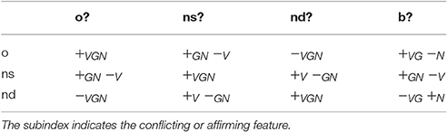
Table 3. Affirmation and challenge of cues by probes; + sign indicates corresponding features, − sign indicates challenge.

Where κ is the parameter expressing affirmation (κ > 0) or challenge κ < 0 of the cue by the probe when the parameter γ_c > 0, and the other way round when γ_c < 0. Multiplication of the driving parameter γ_c leads to a modified composed parameter κ_pγ_c in the Hamiltonian to affirm or mitigate the participant's initial recollection of the cue. We want to emphasize that the second stage Hamiltonians for the probes are thus structured exactly in the same way as the Hamiltonians for the corresponding cues, except that the driving parameters γ are modulated by multiplying them with dedicated tweaking parameters κ.

Reflection following b? probe. While it is not needed in the first reflection stage, under the disjunctive probe b? in the second stage a dedicated Hamiltonian, Equation (22), is still required. Also the Hamiltonian proper to the exposure of the b? probe is based on its target state vector ${(\sqrt{1-|\beta {|}^2},1+\beta ,0)}^{\tau }$. This consists of the actions of H_o(γ_o) and H_ns(γ_ns) where the parameters in the corresponding gates have been added, or subtracted if the transport is in opposite direction¹⁴;

$\begin{array}{l}{H}_b({\gamma }_o,{\gamma }_{ns},\beta )=G_{21}({\gamma }_o\sqrt{1-|\beta {|}^2}-{\gamma }_{ns})+G_{31}({\gamma }_o\sqrt{1-|\beta {|}^2})\\ +G_{32}({\gamma }_{ns}+\beta {\gamma }_o)& (23)\end{array}$

The Hamiltonian for the b? probe thus uses three parameters γ_o, γ_ns and β which it inherits from the Hamiltonians for its component probes o? or ns?.

Unitary evolution and time of measurement. An issue with quantum-like models is the typical appearance of oscillations of probability over time. These oscillations in the evolution are essentially due to the inherent periodicity of a finite dimensional and energetically closed quantum system. Simply put, such systems will always evolve back to their initial state and do over the exact same itinerary in their Hilbert space—ad infinitum. Evidently, in the domain of cognition, when quantum-like modeling of experimental paradigms is done, only within-period evolution should be given meaningful interpretation [24]. In that sense a guideline for the time of measurement would be to keep the reflection times short with respect to the full period. Another option to arrest the characteristic probability oscillation is to include a third stage in the experimental paradigm driven by a ‘grab coat and leave’ Hamiltonian, which would be dedicated to freeze the perceived memory state (set all driving parameters γ equal to zero). More elegantly a termination should be formalized to damp the memory state vector back into its baseline uninformed state by using Lindblad evolution for an open system (e.g., [27, 28] Broekaert et al., under review).

A number of alternative criteria could be put forward to decide this instance of measurement, though at present we keep to an ad hoc cut to the unitary time propagation as proposed by Busemeyer et al. [23] and Busemeyer and Bruza [4]¹⁵. With the intent of the possibility of tweaking the observed acceptance probabilities by description dependence in the second reflection period, we have taken the ad hoc reflection durations of both stages somewhat shorter; $\frac{\pi }{3}$ for each stage.

The first stage ends at $t=\frac{\pi }{3}$, the unitary operator of the second stage picks up there after. The vector of the perceived memory state at time t after probe presentation is then obtained by propagating the initial state, Equation (9), by the concatenated Schrödinger propagators;

$\begin{array}{l}{\Psi }_{p|c}(t)=e^{-i{H}_{p?}t}{e}^{-i{H}_c\frac{\pi }{3}}{\Psi }_0,\text{ and}\\ {\Psi }_0=\frac{1}{\sqrt{3+2\Re (\beta )}}{(\sqrt{1-|\beta {|}^2},(\beta +1),1)}^{\tau }& (24)\end{array}$

Also the second stage ends at $t=\frac{\pi }{3}$, after the first stage. Time evolution prior to the second stage can be obtained by deleting the propagator of the second stage and letting the first propagator have the argument t. The acceptance probabilities p(p?|c) can then be derived using their expressions, Equations (12, 13), in terms of state vector components and will be fitted to the observed data by SSE optimization of the seven free parameters of our Hamiltonian driven QEM model.

3. Fitting the Models to the EOD Data

The data fitted post-hoc parameters for Brainerd et al.'s QEM. QEM provides three amplitudes per cue {v_c, g_c, nd_c}, which satisfy normalization (Equation 5). Therefore six numbers should cover the experimental data sets. Our prescription for acceptance probabilities, Equations (12, 13), coincide with Brainerd et al. [1, p. 243]:

$\begin{array}{l}||M_{O,y}|S_C\rangle |{|}^2=|v_C{|}^2+|g_C{|}^2||M_{ns,y}|S_C\rangle |{|}^2\\ =|g_C{|}^2||M_{ND,y}|S_C\rangle |{|}^2=|n_C{|}^2\end{array}$

and in the same logic we have in QEM, see Equation (7);

$\begin{array}{l}||M_{B,y}|S_C\rangle |{|}^2=||M_{O,y}|S_C\rangle |{|}^2=|v_C{|}^2+|g_C{|}^2.\end{array}$

We notice that in QEM we will always predict p(o?|C) ≥ p(ns?|C), which is of course only the case for the o cue data. Since the modulus square amplitudes are positive numbers, data with p(o?|C) < p(ns?|C) cannot be accommodated in the original version of QEM.

Similarly in the disjunction paradigm QEM would always predict p(o?|C) = p(ns?|C), which is not apparent in the experimental disjunction data (Table 1) and certainly not so for ns and nd cues. Without any other means to fine tune the acceptance probabilities we would expect low accuracy of prediction for them, while we expect pronounced total probability and unpacking factor in the subadditivity paradigm and the disjunction paradigm respectively, Tables 1, 2. Optimized QEM parameters appear in Tables 4, 5.

TABLE 4

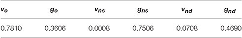
Table 4. EOD-disjunction paradigm: Optimized fit of independent QEM parameters providing RMSE = 0.1112, ($v_c,g_c\in {ℝ}^{+}$).

TABLE 5

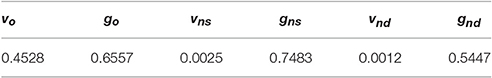
Table 5. EOD-subadditivity paradigm: Optimized fit of independent QEM parameters providing RMSE = 0.0963, ($v_c,g_c\in {ℝ}^{+}$).

The data fitted parameters of the Feynman path based model. The Feynman path model required six parameters to obtain the nine acceptance probabilities of disjunction paradigm ([4], Ch. 6). The model allows to reproduce very well the general required pattern of acceptance probabilities at RMSE = 0.0298, which turn out the precise EOD effects, except for the new dissimilar cues {nd}, Table 1. In the latter case the unpacking factor turns out smaller than 1, i.e., the conjunction value turns out negative.

The Feynman path model was not adapted yet to the subadditivity paradigm, but since it uses interference of amplitudes and reversed gist/verbatim processing depending on the type of cue, the model should be applicable in that paradigm as well.

The data fitted Hamiltonian driven QEM parameters. With both experiments reporting different data for similar expressions, we have fitted the Hamiltonian model to each separately¹⁶. For the EOD-disjunction paradigm the model obtained closely fitted parameters to the experimental data, with RMSE = 0.0073 with β > 0. When β < 0 constraint was imposed a less good RMSE = 0.0341 was obtained. The nine predicted probabilities p(p?|c) by the parameters of Table 6 are shown in Table 1.

TABLE 6

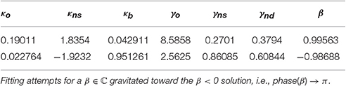
Table 6. EOD-disjunction paradigm: Optimized fit of Hamiltonian parameters under β > 0 (RMSE = 0.0073), and β < 0 (RMSE = 0.0341) constraint.

For the EOD-subadditivity paradigm the model obtained a less efficient fit of parameters to the experimental data, with RMSE = 0.0565 for β > 0. When β < 0 the parameter fit allowed an improved RMSE = 0.0191. The Hamiltonian model for the EOD-paradigm allowed a very good data fit using complex β at RMSE = 0.0032. We recall that complex numbers consist of a modulus and a phase, therefore one complex parameter should actually be counted as two real parameters. We shortly comment on this issue in the discussion, Section 4. The nine predicted probabilities p(p?|c) following the parameters of Table 7 for the three cases are shown in Table 2.

TABLE 7

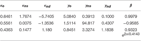
Table 7. EOD-subadditivity paradigm: Optimized fit of Hamiltonian parameters under constraint β > 0 (RMSE = 0.0565), β < 0 (RMSE = 0.0191) and β ∈ ℂ (RMSE = 0.0032).

The temporal evolution of acceptance probabilities. With the optimized values of the driving parameters calculated, the temporal progression of the acceptance probability can be graphed (Figures 1–5). The dashed lines represent the first-stage evolutions when the participant is shown the cue for recognition, while the full lines represent the second-stage evolutions when the probes enquire for accepting the type of a cue. The ultimate instance of measurement happens at the end of the second stage (t = 2π/3). In all graphs, in the first stage the color indicates the “probability value” of the traces; red codes for perceiving the cue's unrelated features (N), orange codes for perceiving the cue's gist (G) and green codes for perceiving the cue's verbatim and gist (V + G)—one can quickly check that for the same cue the dashed red and dashed green values add up to 1 at each moment in the first stage. Evidently these first stage “probability values” should not be conflated with the participants acceptance probabilities. Only after the probe has enquired the participant do these values evolve as the nine acceptance probabilities. It is worthwhile to note that the optimalization of parameters has returned initial states which either contain no gist or no verbatim perception in the cases with real-valued β (at t = 0 respectively; orange has almost value zero or, green and orange almost coincide). Only when β is complex-valued does the initial value show substantial gist and verbatim trace. We have provided two graphs for the EOD-disjunction paradigm (Figures 1, 2) the first one was constrained to have β > 0 while the second had to satisfy β < 0. In this EOD-disjunction paradigm no complex-valued β offered an optimized fit. For the EOD-subadditivity paradigm we provide three graphs (Figures 3–5), respectively with the constraints β > 0, β < 0, and β ∈ ℂ.

FIGURE 1

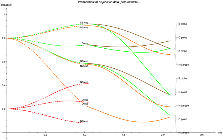
Figure 1. β > 0 case: temporal evolution of acceptance probabilities for the EOD-disjunction paradigm [3]. Red indicates N probability component, orange indicates G probability component and green indicates V + G probability component. In the second stage brown indicates the acceptance probability for the b? probe (V + G). Notice the near absence of verbatim in the initial state.

FIGURE 2

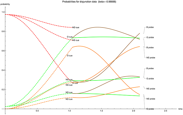
Figure 2. β < 0 case: temporal evolution of acceptance probabilities for the EOD-disjunction paradigm [3]. Red indicates N probability component, orange indicates G probability component while green indicates V + G probability component. In the second stage brown indicates the acceptance probability for the b? probe (V + G). Notice the near absence of gist in the initial state.

FIGURE 3

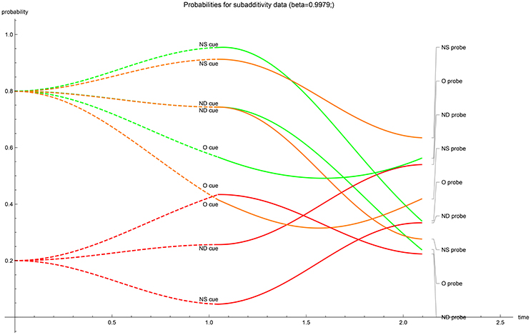
Figure 3. β > 0 case: temporal evolution of acceptance probabilities for the EOD-subadditivity paradigm [1]. Red indicates N probability component, orange indicates G probability component while green indicates V + G probability component. Notice the near absence of verbatim in the initial state.

FIGURE 4

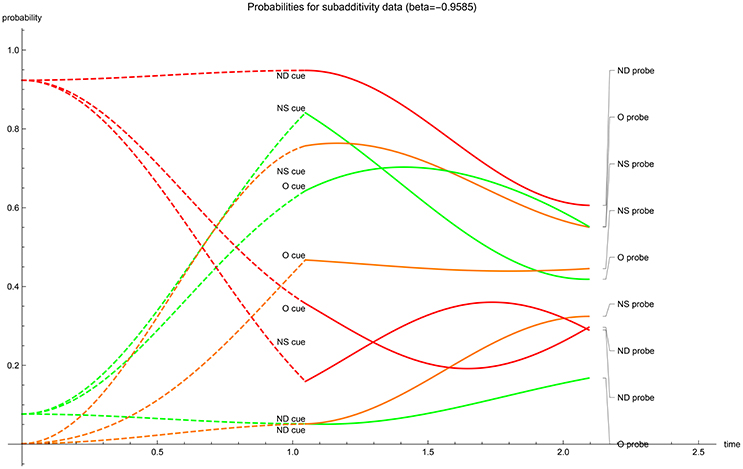
Figure 4. β < 0 case: temporal evolution of acceptance probabilities for the EOD-subadditivity paradigm [1]. Red indicates N probability component, orange indicates G probability component while green indicates V + G probability component. Notice the near absence of gist in the initial state.

FIGURE 5

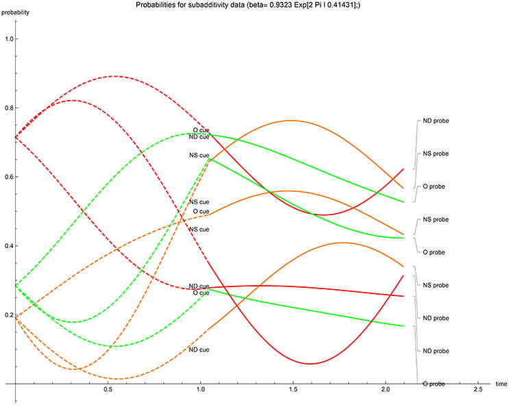
Figure 5. β ∈ ℂ case: temporal evolution of acceptance probabilities for the EOD-subadditivity paradigm [1]. Red indicates N probability component, orange indicates G probability component while green indicates V + G probability component. Notice both verbatim and gist are present in the initial state.

One observes that in the first stage the dynamics is mostly monotonic—except for the one case where β ∈ ℂ (Figure 5). In the second stage dynamics some intermediary extrema do appear, which from a cognitive point of view are not to be expected. The factor of description dependence was expected to be a smaller modification of the first stage recognition. The second stage extrema however need to be understood with respect to the ad hoc instance of measurement at t = π/3 after enquiry, adopting a shorter measurement time could have mitigated this temporal behavior. Finally we note that also the outspoken VGN spread of the initial vector could be related to a too extended period for evolution. While the fitting of the experimental acceptance probability data in the Hamiltonian driven QEM has shown good accuracy, the concomitant intermediate temporal evolution leaves room for improving the measurement protocol.

4. Discussion

We had set out to develop a Hamiltonian driven model that would provide temporal evolution of the memory state of the Quantum Episodic Model of Brainerd et al. [1, 9]. The model uses nine different state vectors for the three cues crossed with three probe paradigms, and requires six parameters to drive the Hamiltonians and one parameter to tweak the gist in the initial state. We provided psychological interpretation of the parameters fitting the experimental process. Initially the memory state prior to cue and probe presentation is an equally weighed mix of o, ns and nd states leading to an overall amount of the gist component monitored by the parameter β. In first stage the ability to recognize the type of the cue c is driven by the cue-specific parameter γ_c in the Hamiltonian. In the second stage the instruction probe p? engenders an amplified or mitigated evolution driven by the probe-specific parameter κ_p for description-dependence.

Our Hamiltonian driven account of QEM shows that the subadditivity and disjunction fallacy are not a priori guaranteed or “parameter free” in our model. The occasions in which these effects would not occur are however very improbable in practice, Equations (14, 15). This possibility is due to the fact that the two-staged Hamiltonian evolution produces nine state vectors Ψ_probe|cue(t) instead of regular QEM's three cue-dependent state vectors Ψ_cue.

Using two reported experimental data sets showing subadditivity and over-distribution of the disjunction in acceptance probabilities for episodic memory recollection, we were able to provide parameter values with good prediction capacity in the Hamiltonian model. In practice we provided values for seven parameters {κ_o, κ_ns, κ_nd, γ_o, γ_ns, γ_nd, β} to predict nine acceptance probabilities {p_o?o, p_ns?o, p_nd?o, p_o?ns, p_ns?ns, p_nd?ns, p_o?nd, p_ns?nd, p_nd?nd} in the subadditivity paradigm and did the same for the disjunction paradigm, Tables 6, 7. Rigorously one should discern the parametrization case when β ∈ ℂ, which should be counted for two parameters even if the function of the real and imaginary part of the parameter take the same position in the model. The present model thus uses one extra parameter in comparison to the Feynman path model of Busemeyer and Bruza but provides better EOD prediction for all type of cues. Moreover the parameters in the Hamiltonian model do allow psychological interpretation. The predictions of acceptance probabilities following the original QEM formulation by Brainerd et al. showed to be flawed by systematic features. In the disjunction paradigm QEM's acceptance probabilities for the both?-probe and the old?-probe can only be identical, and in both experimental paradigms QEM's acceptance probability for the old?-probe can only be larger than or equal to the acceptance probability for the new-similar?-probe, whatever the cue type.

The issue of “description-dependence” effect seems crucial in obtaining final acceptance probabilities; the κ factors are rather large in comparison to the driving parameters γ and cause outspoken evolution in second stage. This fact is rather counter intuitive as a priori we had expected small corrective modulation in second stage evolution (see Tables 6, 7, Figures 1–5).

We found it remarkable that β ≈ ± 1 is needed for best fit in both experimental paradigms when keeping β ∈ ℝ. This would suggest that the verbatim trace is almost negligible in comparison to the gist in the set of true cues {o} in the initial state, or just the inverse. When β is allowed to be complex a mix of both traces is present in the best fitting initial state for the EOD-subadditivity paradigm. In the EOD-disjunction paradigm complex β did not provide a best fit (the limit value became real).

Superposed Hadamard gates with off-diagonal parameters show to be a viable method in the construction of Hamiltonians. The “description-dependence” factor κ can indeed mitigate probability oscillations. The best example can be seen in the β < 0 subadditivity Graph 4 where a small κ_o = 0.022764 acts on an average γ_o = 2.5625 and gives in the second stage nearly unmodulated continuation for p_o?|o(t), p_o?|ns(t) and p_o?|nd(t) (solid green lines).

The ad hoc time $\frac{\pi }{3}$ avoided most intermediate extrema in the probabilities in the second reflection stage, except for β ∈ ℂ. We remark that lower time of measurement could bring about the problem of not being able to spread open to a range of probabilities in time when starting from some pre-defined—e.g., equal– probability configuration, or just trade of with ever growing driving parameters γ. A longer time of measurement would increase the well-known issue of intermediate extrema.

We have used the equally weighed initial state $1/{N}{\left[\sqrt{1-|\beta {|}^2},1+\beta ,1\right]}^{\tau }$ in VGN space to give each vector |o〉, |ns〉 and |nd〉 equal weight at start which we consider reflected best the information communicated by the experimenter. The optimized data fit shows e.g., β ≈ ± 1 in both paradigms with the perceived implicit probabilities at the start at p(o) ≈ 0.8, p(ns) ≈ 0.8 and p(nd) ≈ 0.2. Which one can observe at t = 0 in both the subadditivity paradigm (Figure 3) and disjunction paradigm (Figure 1). The precise nature of the initial vector for the memory state of the participant after studying {o} and having heard ‘all type of cues will be presented with equal probability’ but prior to cue and probe presentation remains somewhat puzzling.

In sum we consider to have constructed an acceptable Hamiltonian driven QEM version, with good prediction capacity for acceptance probabilities. Future work could include covering the model fitting of a data set which covers both the subadditivity and disjunction paradigm at once –eight parameters for twelve datapoints– to verify its further prediction capacity, and to monitor more closely the initial memory state in the experimental paradigms and the meaurement protocol.

Author Contributions

JBB has designed the Hamiltonian model for the EOD paradigm and provided data fitting and interpretation. JRB is the author of the Feynman path model for the EOD-paradigm and provided prior knowledge on the QEM model and Hamiltonian design, and did critical revision of the work.

Conflict of Interest Statement

The authors declare that the research was conducted in the absence of any commercial or financial relationships that could be construed as a potential conflict of interest.

Acknowledgments

JBB gratefully thanks JRB for extensive discussions on Hamiltonian and Markov dynamical decision models and their relation to the EOD effect, and also thanks Cole Rodman for insightful discussions on 3 × 3 categorization-decision paradigms in quantum-like modeling. This work was made possible by FWO-Vlaanderen mobility grant V410016N. Further thanks go to an reviewer for inciting clarifications.

Footnotes

1. ^We adopted the notation of Brainerd et al. [1] in the context of Brainerd et al. [3] as well. Always cues will be denoted o, ns, and nd for old, new-similar, and new-dissimilar, and their respective enquiring probes are o?, ns?, and nd?. Memory traces are denoted by V, G, and N for verbatim, gist, and neither.

2. ^In the conjoint recognition model the probabilities for acceptance for unrelated distractors are: p_u,T = b_T, p_u,R = b_R, and p_u,T+R = b_T+R, (9, Equations 19–21).

3. ^We use the symbol τ to designate the transpose of a vector or matrix. Basically transposition turns columns into rows and vice versa.

4. ^We recall that state functions or vectors in quantum-like models for cognitive processes will always represent averages of the participant group. Individual memory state vectors are not envisaged in this approach: as all humans are allegedly equal but rather existentially different the average state function does not reflect the individual's memory state. We emphasize the difference with the situation in the micro-physical realm; e.g., the state function of an ensemble of identically prepared electrons does reflect the behavior of an individual electron since all electrons are equal, not just allegedly.

5. ^Brainerd et al. [1, p. 239], mentions participants would have roughly p(o) = p(ns) = p(nd) = 1/3 as baseline probabilities prior to study of {o}. Let the initial state be represented in VGN space as (α, β, γ)^τ. Using the appropriate projection operators, Equation(6), we find p(o) = |α|² + |β|², p(ns) = |β|² and p(nd) = |γ|². Equating them all to 1/3 requires α = 0, reducing the perceived related verbatim trace to nought.

6. ^An explicit eigenvector |o(α, β)〉 of M_y,o? is given by $M_{y,o?}|o(\alpha ,\beta )\rangle =|o(\alpha ,\beta )\rangle ={[\alpha ,\beta ,0]}^{\tau }=\alpha |V\rangle +\beta |G\rangle$, with |α|² + |β|² = 1. Evidently there is a possible denomination issue caused by the relative weight of both components, since diminishing α will eventually turn an o state indiscernibly into an ns state.

7. ^The equally weighed initial state $1/{N}{(\sqrt{1-|\beta {|}^2},1+\beta ,1)}^{\tau }$ was obtained by giving each type of cue's vector |o〉, |ns〉 and |nd〉 equal weight at start. Our implementation however does neither reflect equal baseline probability of o, ns, and nd in the participants memory state as aimed for by Brainerd et al. [1], also here one cannot have p(o) = p(ns) = p(nd) at the start. For real-valued β, the initial probabilities come at the closest for $\beta =-2+\sqrt{3}$ at p_o = 0.59, p_ns = 0.22, p_nd = 0.41.

8. ^The original notation V for “verbatim,” R for “related,” and U for “unrelated” cues are here replaced by o, ns, and nd, respectively. One should be attentive to the fact that V stood for “is the cue verbatim?” (actually meaning old), it does not stand for the verbatim trace of QEM.

9. ^Meaning probe-dependence by differing κ_b and κ_o in the second stage propagation.

10. ^Brainerd et al. [1, p. 19]) mentions: “[…] a distinct memory state vector is generated for each of the three types of cues, with corresponding amplitudes v_C, g_C, and n_C.” (see Equations 4, 5). Our present Hamiltonian take of the QEM structure provides nine memory state vectors. Starting from one single initial state our Hamiltonian dynamics provides a distinct state vector for each of the nine configurations of the three cues crossed with the three probes. Therefore we have nine normalization conditions of the vectors (Equation 11), and can have some modulation in the unpacking factor and in the subadditivity expression.

11. ^Applying the Hamiltonian to the initial state gives a first-order approximation of the change of the state vector for an infinitesimal time interval:

$\begin{array}{l}{\psi }_{\delta t}-{\psi }_0\approx \frac{i\delta t}{\hslash }H{\psi }_0\end{array}$

This allows us to design the Hamiltonian according the needs of the cognitive process.

12. ^E.g.,:

$\begin{array}{lll}{G}_{21}(h)=\frac{1}{\sqrt{1+|h{|}^2}}\left(\begin{array}{ccc}1& h& 0\\ h^{\star }& -1& 0\\ 0& 0& 0\end{array}\right)& \text{with}& G_{21}{(h)}^2=\left(\begin{array}{ccc}1& 0& 0\\ 0& 1& 0\\ 0& 0& 0\end{array}\right).\end{array}$

This modification retains the rotation effects of the operator and squares to the unity operator in VG-space. A main advantage of the present form is the oscillations of probability over time stop when the parameter is set equal to zero.

13. ^With β a complex number one must take care to keep the Hadamard gate Hermitian.

14. ^One must take into account G₁₂(γ) = −G₂₁(−γ).

15. ^Choice $t=\frac{\pi }{2}$ corresponds to a first extremum when significant parameters in the Hamiltonian are set equal to zero, i.e., when the actual psychological dynamics is “turned off” in the model.

16. ^Matlab's fmincon function on SSE was used with a 3⁶2¹ (β ∈ ℝ) or 3⁶2² (β ∈ ℂ) grid for the initial vector in the parameter space.

References

1. Brainerd CJ, Wang Z, Ryena VF, Nakamura K. Episodic memory does not add up: verbatim-gist superposition predicts violations of the additive law of probability. J Mem Lang. (2015) 84:224–45. doi: 10.1016/j.jml.2015.06.006

CrossRef Full Text | Google Scholar

2. Brainerd CJ, Reyna VF. Episodic over-distribution: a signature effect of familiarity without recollection. J Mem Lang. (2008) 58:765–86. doi: 10.1016/j.jml.2007.08.006

CrossRef Full Text | Google Scholar

3. Brainerd CJ, Reyna VF, Aydin C. Remembering in contradictory minds: disjunction fallacies in episodic memory. J Exp Psychol Learn Mem Cogn. (2010) 36:711–35. doi: 10.1037/a0018995

PubMed Abstract | CrossRef Full Text | Google Scholar

4. Busemeyer JR, Bruza PD. Quantum Models of Cognition and Decision Making. Cambridge, UK: Cambridge University Press (2012).

5. Tulving E. Episodic and semantic memory. In: Tulving E, Donaldson W, editors. Organization of Memory. New York, NY: Academic Press (1972). p. 381–402.

6. Mandler G. Recognizing: the judgment of previous occurrence. Psychol Rev. (1980) 87:252–71.

Google Scholar

7. Tulving E. Precis of elements of episodic memory. Behav Brain Sci. (1984) 7:223–68. doi: 10.1017/S0140525X0004440X

CrossRef Full Text | Google Scholar

8. Jacoby LL. A process dissociation framework: separating automatic from intentional uses of memory. J Mem Lang. (1991) 30:513–41.

Google Scholar

9. Brainerd CJ, Reyna VF, Mojardin AH. Conjoint recognition. Psychol Rev. (1999) 106:160–79. doi: 10.1037/0033-295X.106.1.160

PubMed Abstract | CrossRef Full Text | Google Scholar

10. Reyna VF, Brainerd CJ. Fuzzy-trace theory: an interim synthesis. Learn Individ Diff. (1995) 7:1–75. doi: 10.1016/1041-6080(95)90031-4

CrossRef Full Text | Google Scholar

11. Brainerd CJ, Wang Z, Reyna VF. Superposition of episodic memories: overdistribution and quantum models. Top Cogn Sci. (2013) 5:773–99. doi: 10.1111/tops.12039

PubMed Abstract | CrossRef Full Text | Google Scholar

12. Brainerd CJ, Holliday RE, Nakamura K, Reyna VF. Conjunction illusions and conjunction fallacies in episodic memory. J Exp Psychol Learn Mem Cogn. (2014) 4:1610–23. doi: 10.1037/xlm0000017

CrossRef Full Text | Google Scholar

13. Nelson DL, Kitto K, Galea D, McEvoy CL, Bruza PD. How activation, entanglement, and searching a semantic network contribute to event memory. Mem Cogn. (2013) 41:797–819. doi: 10.3758/s13421-013-0312-y

PubMed Abstract | CrossRef Full Text | Google Scholar

14. Bruza P, Kitto K, Nelson D, McEvoy C. Is there something quantum-like about the human mental lexicon? J Math Psychol. (2009) 53:362–77. doi: 10.1016/j.jmp.2009.04.004

PubMed Abstract | CrossRef Full Text | Google Scholar

15. Brainerd CJ, Reyna VF, Holliday RE, Nakamura K. Overdistribution in source memory. J Exp Psychol Learn Mem Cogn. (2012) 38:413–39. doi: 10.1037/a0025645

PubMed Abstract | CrossRef Full Text | Google Scholar

16. Tversky A, Koehler DJ. Support theory; A nonextensional representation of subjective probability. Psychol Rev. (1994) 101:547–67.

Google Scholar

17. Denolf J. Subadditivity of episodic memory states: a complementarity approach. In: Atmanspacher H, Bergomi C, Filk T, Kitto K, editors. Lecture Notes in Computer Science, Vol. 8951. Cham: Springer (2015). p. 67–77. doi: 10.1007/978-3-319-15931-7_6

CrossRef Full Text | Google Scholar

18. Denolf J, Lambert-Mogiliansky A. Bohr complementarity in memory retrieval. J Math Psychol. (2016) 73:28–36. doi: 10.1016/j.jmp.2016.03.004

CrossRef Full Text | Google Scholar

19. Batchelder WH, Riefer DM. Multinomial processing models of source monitoring. Psychol Rev. (1990) 97:318–39. doi: 10.1037/0033-295X.97.4.548

CrossRef Full Text | Google Scholar

20. Bayen UJ, Murnane K, Erdfelder E. Source discrimination, item detection, and multinomial models of source monitoring. J Exp Psychol Learn Mem Cogn. (1996) 22:197–215. doi: 10.1037/0278-7393.22.1.197

CrossRef Full Text | Google Scholar

21. Deese J. On the prediction of occurrence of certain verbal intrusions in free recall. J Exp Psychol. (1959) 58:17–22. doi: 10.1037/h0046671

CrossRef Full Text

22. Roediger HL, III, McDermott KB. Creating false memories: Remembering words not presented on lists. J Exp Psychol Learn Mem Cogn. (1995) 21:803–14. doi: 10.1037/0278-7393.21.4.803

CrossRef Full Text | Google Scholar

23. Busemeyer JR, Trueblood J. Quantum model for conjoint recognition. In: Quantum Informatics for Cognitive, Social, and Semantic Processes: Papers from the AAAI Fall Symposium. Arlington, VA: Association for the Advancement of Artificial Intelligence (2010).

Google Scholar

24. Broekaert J, Aerts D, D'Hooghe B. The generalized liar paradox: a quantum model and interpretation. Found Sci. (2006) 11:399–418. doi: 10.1007/s10699-004-6248-8

CrossRef Full Text | Google Scholar

25. Yearsley JM, Pothos EM. Zeno's paradox in decision-making. Proc R Soc N (2016) 283:20160291. doi: 10.1098/rspb.2016.0291

PubMed Abstract | CrossRef Full Text | Google Scholar

26. Aerts D, Broekaert J, Smets S. A quantum structure description of the liar-paradox. Int J Theor Phys. (2000) 38:3231–9. doi: 10.1023/A:1026686316673

CrossRef Full Text | Google Scholar

27. Asano M, Ohya M, Tanaka Y, Basieva I, Khrennikov A. Quantum-like model of brain's functioning: decision making from decoherence. J Theor Biol. (2011) 281:56–64. doi: 10.1016/j.jtbi.2011.04.022

PubMed Abstract | CrossRef Full Text | Google Scholar

28. Khrennikova P, Haven E, Khrennikov A. An application of the theory of open quantum systems to model the dynamics of party governance in the US Political System. Int J Theor Phys. (2014) 53:1346–60. doi: 10.1007/s10773-013-1931-6

CrossRef Full Text | Google Scholar