Toward First Principle Medical Diagnostics: On the Importance of Disease-Disease and Sign-Sign Interactions

1. Introduction

Human body as a whole or in part may adopt various states, like a Rubik's Cube. Homeostatic mechanisms, medical interventions and aging all involve evolution from certain body states to others. Similarly, evolution of states is commonly seen in cells that constitute our bodies. Immune cells for example can manifest substantial plasticity and develop into distinct phenotypes with different functions [1, 2]. Identifying dysfunctional states in cells is in many ways similar to identifying diseases in organisms and is confronted by similar difficulties. State assignment, as we describe below, is often a nontrivial and challenging process and in many cases it is hard to “diagnose” the state of a cell or conditions of a patient. The progress in systems biology and availability of large data has made diagnostics even more challenging. For instance, mass cytometric analysis of immune cells has led to identification of many new cell subtypes (states) [3]. Metabolomic analysis of cells and body fluids revealed a large number of biomarkers and disease subtypes [4]. There is a huge need in the fields of cell biology, immunology, clinical sciences and pharmaceutical sciences for approaches to identify states, assigning states and characterizing co-emerging or co-existing states. Moreover, it is often important to be able to identify emerging states even before they are fully evolved. From physics point of view, it is interesting to yield a generic understanding of the state assignment problem in cell biology or medicine (although specific details might be crucial in each context in practice). Without loss of generality, in what follows we focus on medical diagnostics and draw a simple picture that captures many generic aspects of assignment problems in medicine and systems cell biology.

Decision-making is at the heart of medicine. Decisions are made at various stages in clinical practice, particularly during diagnostic investigations and when assigning the findings to a disease [5, 6]. Diagnostic strategies are typically available in the form of clinical algorithms and flow charts that define the sequence of actions to be taken to reach a diagnosis. The diagnosis itself is typically made based on consensus diagnostic criteria [7, 8]. In addition, there are a number of clinical decision support systems and software systems that are used to assign findings (symptoms and signs) to disease conditions. The most commonly used technologies are WebMD Symptom Checker, Isabel Symptom Checker, DXplain and Internist [9]. These algorithms compute the most likely disease that is associated with a given set of findings by using only a small part of the existing probabilistic data on findings and diseases. Internist, which is one of the most sophisticated systems, relies on two parameters, the probability of a finding given a disease and the probability of a disease given a finding [10]. These technologies inform us if a patient satisfies the criteria of a disease but do not provide guidance on how to approach a patient and mostly ignore the interactions between diseases.

Currently, we lack a solid conceptual framework for medical diagnostics. As a consequence, there is no consensus on the diagnostic flow charts available today, and clinicians differ widely in their approaches to patients. Here, we take a step toward solving this problem by formulating first principles medical diagnostics. We evaluate the performance of the platform and discuss how one can optimize it. Using simple theoretical examples, we show how including relevant statistical data and often-ignored inherent disease-disease linkages significantly reduces diagnostic errors and mismanagement and enables the early diagnosis of disease.

The problem of associating a subset of observed signs (clinical signs/symptoms and laboratory data) with specific diseases was easy if we could assume the findings originate from a single disease, we had clear demonstrations for the diseases, and inter-sign and inter-disease interactions were negligible. In practice, however, we typically have no certain relationships that connect signs to diseases, and one often must address interference effects of multiple diseases; in the early stages of a disease, we do not even have sufficient findings to make a definite decision [11–13]. There are a number of studies that have attempted to quantify such dependencies under uncertainty and obtain estimations for the likelihood of diseases given a subset of findings [10, 14–19]. An essential simplifying assumption in these studies was that only one disease is behind the findings (exclusive diseases assumption), otherwise, the diseases act independently on the symptoms (causal independence assumption). Among recent developments, we should mention Bayesian belief networks, which provide a probabilistic framework to study sign-disease dependencies [20–23]. These models are represented by tables of conditional probabilities that show how the state of a node (sign or disease) variable in an acyclic directed graph depends on the state of the parent variables. Here, it is usually assumed that the signs are conditionally independent of one another given a disease hypothesis and that diseases are independent of one another after marginalizing over the sign variables (marginally independent diseases). In other words, there exist no causal dependencies or interactions (directed links in the graph) that connect two signs or diseases. Then, starting from the conditional probabilities of the sign variables, the posterior disease probabilities are obtained by the Bayes' rule using the above simplifying assumptions [21].

In this study, however, we shall pursue a more principled approach to highlight the significance of direct disease-disease and sign-sign interactions (dependencies). Evidences are rapidly growing to support the existence of such interactions [24–31]. We construct a probabilistic model of interacting sign and disease variables which goes beyond the assumptions that mentioned in the previous paragraph; specifically, here the effects of the diseases on the symptoms can be correlated, and more than one disease can be involved in the study. In addition, in the presence of the sign-sign interactions, the value of one observed sign can affect the belief on the value of another unobserved sign. The price we pay in return is to deal with the techniques of model learning, to obtain the model parameters from statistical relations of the sign and disease variables. And, we have to employ more sophisticated inference algorithms, to estimate the marginal sign and disease probabilities from the model. Our approach is of course computationally more expensive than the previous approaches, but it shows how different types of interactions could be helpful in the course of diagnosis. Additionally, because of recent developments in related fields [32–35], we now have the necessary concepts and tools to address difficulties in more sophisticated (realistic) problems of this type. This study does not involve usage of real medical data, which is by the way fundamentally incomplete at this moment for such modeling; however, it provides a rationale as to why certain often-neglected statistical information and medical data can be useful in diagnosis and demonstrates that investments in collecting such data will likely pay off.

2. Problem Statement

Consider a set of N_D binary variables D = {D_a = 0, 1 : a = 1, …, N_D}, where D_a = 0, 1 shows the absence or presence of disease a. We have another set of N_S binary variables S = {S_i = ±1 : i = 1, …, N_S} to show the values of sign (symptom) variables. A sign here could stand for a medical test, history, or the state of a biomarker (e.g., protein, metabolite, gene).

Suppose we have the conditional probability of symptoms given a disease hypothesis, P(S|D), and prior probability of diseases P₀(D). Then, the joint probability distribution of sign and disease variables reads as P(S; D) ≡ P(S|D)P₀(D). We shall assume, for simplicity, that the probability distributions describe the stationary state of the variables. The distributions may be subject to environmental and evolutionary changes and may also change in the course of the disease. Here, we limit our study to the time scales that are smaller than the dynamical time scale of the model and leave the temporal dynamics for a future study. In addition, we assume that we are given sufficient statistical data, e.g., the true marginal probabilities P_true(S_i, S_j|D), to reconstruct simple models of the true probability distribution [36]. This is indeed the first part of our study: In Section 3.1, we propose statistical models of sign and disease variables, and employ efficient learning algorithms to compute the model parameters, given the appropriate data. Fortunately, recent advances in machine learning and inference techniques enable us to work with models that involve very large number of variables [35, 37–44].

Let us assume that a subset O = {i₁, i₂, …, i_NO} of the sign variables has been observed with values S^o, and size N_O = |O|. We will use U for the remaining subset of unobserved signs with values which are denoted by S^u. Then, the likelihood of disease variables given the observed signs is:

$\begin{array}{ll}{L}(\text{D}|{\text{S}}^o)\equiv {\displaystyle \sum _{{\text{S}}^u}}P(\text{S};\text{ D}).& (1)\end{array}$

The most likely diseases are obtained by maximizing the above likelihood:

$\begin{array}{ll}{\text{D}}_{ML}=arg{\displaystyle \underset{\text{D}}{max}}log{L}(\text{D}|{\text{S}}^o).& (2)\end{array}$

Here, we are interested in the posterior probability marginals P(D_a = 0, 1) of the disease variables. The marginal probability P(S_j = ±1) of an unobserved sign, and the most likely signs, are obtained from the following distribution:

$\begin{array}{ll}{M}({\text{S}}^u|{\text{S}}^o)\equiv {\displaystyle \sum _{\text{D}}}P(\text{S};\text{ D}),{\text{S}}_{ML}=arg{\displaystyle \underset{{\text{S}}^u}{max}}log{M}({\text{S}}^u|{\text{S}}^o).& (3)\end{array}$

The main task in the second part of our study is computation of the sign and disease marginal probabilities

$\begin{array}{ll}P(D_a)\propto {\displaystyle \sum _{\left\{D_b:b\ne a\right\}}}{L}(\text{D}|{\text{S}}^o),P(S_j)\propto {\displaystyle \sum _{\left\{S_k:k\in U\backslash j\right\}}}{M}({\text{S}}^u|{\text{S}}^o)j\in U.& (4)\end{array}$

In general, computing the exact values of these marginals is a hard problem. However, one can find highly accurate approximation methods developed in the artificial intelligence and statistical physics communities to address such computationally difficult problems [32, 33, 45–48]. In Section 3.2, we propose an approximate message-passing algorithm for inferring the above information in a large-scale problem.

Finally, the last and main part of our study is devoted to the problem of choosing a finite sequence of unobserved signs for observation, which maximizes an appropriate objective functional of the sequence of observations. In principle, the objective function should be designed to approach the right diagnosis in a small number of observations. To this end, we assign larger values to the objective function if the observations result to larger polarization in the disease probabilities; obviously, it is easier to decide if disease a is present or not when the marginal probability P(D_a) is closer to 0 or 1 (more polarized). Computing such an objective functional of the disease probabilities for a given sequence of observations is not an easy task. We have to consider also the stochastic nature of the observations; we know the sign probabilities P(S_j), but, we do not know a priori the value S_j of an unobserved sign, which is chosen for observation. To take into account this uncertainty, we shall work with an objective function which is averaged over the possible outcomes of the observation. More precisely, the above diagnosis problem is a multistage stochastic optimization problem, a subject that has been extensively studied in the optimization community [34, 49–51].

Suppose we are to observe T ≤ N_S − N_O signs with an specified order O_T ≡ {j₁, …, j_T}; there are (N_S − N_O)!/(T!(N_S − N_O − T)!) different ways of choosing T signs from N_S − N_O ones, and T! different orderings of the selected signs to identify such a sequence of observations. Therefore, the number of possible sequences grows exponentially with T. Add to this the computational complexity of working with an objective functional of the sequence of observations, which has to be also averaged over the stochastic outcomes of the observations. In Section 3.3, we present simple heuristic and greedy algorithms to address the above problem, and leave a detailed study of the multistage stochastic optimization problem for future.

3. Results

A complete description of a collection of stochastic variables, like the sign and disease variables, is provided by the joint probability distribution of the variables P(S; D). Having the probability distribution (model) that describes a system of interacting variables does not, however, mean that one can readily extract useful statistical information from the model. In fact, both the model construction and the task of extracting information from the model are computationally hard, with computation times that in the worst cases grow exponentially with the number of involved variables [52–56]. In the following, we address the above sub-problems in addition to the main problem of optimizing an appropriate objective functional of observations, which are made during the course of diagnosis.

3.1. Learning the Model: Maximum Entropy Principle

Let us assume that we are given the marginal probabilities P_true(S_i, S_j|D) of the true conditional probability P_true(S|D); we consider at most the effects of two-sign interactions, which is expected to capture a significant part of the behavior that arises from interactions between the sign variables. Moreover, the strength of the higher order interactions is expected to be smaller than one-sign and two-sign interactions. And, it would be much more difficult to obtain clinical data of good statistical quality to reconstruct such interactions. Given the true marginal probabilities, we use the maximum entropy principle to construct an appropriate model P(S; D) ≡ P(S|D)P₀(D) of the sign and disease variables [57–59]. Here, P₀(D) is the prior probability of the diseases depending on the age, gender, and other characteristics. Here, we simply take a product prior distribution, P₀(D) = ∏_aP₀(D_a). In the absence of any prior information, the above probability distribution is uniform.

The conditional probability P(S|D) represents all the sign/disease interactions that are allowed by the maximum entropy principle,

$\begin{array}{ll}P(\text{S}|\text{D})=\frac{1}{Z(\text{D})}exp\left({\displaystyle \sum _i}{h}_i(\text{D})S_i+{\displaystyle \sum _{i<j}}{J}_{ij}(\text{D})S_i{S}_j\right).& (5)\end{array}$

Here Z(D) is the normalization (or partition) function.

In practice, we are given only a small subset of the conditional probabilities, for instance, P_true(S_i, S_j|onlyD_a) and P_true(S_i, S_j|onlyD_a, D_b). The former is the probability that signs i and j take values (S_i = ±1, S_j = ±1) conditioned to the presence of disease a and the absence of all other diseases. The latter conditional probabilities are defined similarly. Therefore, we have to consider only interactions between a small number of disease variables. To this end, we expand the model parameters,

$\begin{array}{ll}{h}_i(\text{D})=h_i^0+{\displaystyle \sum _a}{h}_i^a{D}_a+{\displaystyle \sum _{a<b}}{h}_i^{ab}{D}_a{D}_b+\cdots ,& (6)\end{array}$

$\begin{array}{ll}{J}_{ij}(\text{D})=J_{ij}^0+{\displaystyle \sum _a}{J}_{ij}^a{D}_a+{\displaystyle \sum _{a<b}}{J}_{ij}^{ab}{D}_a{D}_b+\cdots ,& (7)\end{array}$

and keep only the leading terms of the expansion. Putting all together, given the above information, we rewrite

$\begin{array}{ll}P(\text{S}|\text{D})=\frac{1}{Z(\text{D})}{\varphi }_0(\text{S})\times {\displaystyle \prod _a}{\varphi }_a(\text{S}|D_a)\times {\displaystyle \prod _{a<b}}{\varphi }_{ab}(\text{S}|D_a,D_b).& (8)\end{array}$

Here, ϕ₀ is responsible for the leak probabilities P(S|nodisease), to account for the missing disease information and other sources of error [21, 23]. In the following, we assume that local sign fields are sufficient to produce an accurate representation of the leak probabilities, i.e., ${\varphi }_0=exp(\sum _i{K}_i^0{S}_i)$. The other interaction factors, ϕ_a and ϕ_ab, are present only if the associated diseases are present; they are written in terms of local sign fields and two-sign interactions:

$\begin{array}{ll}{\varphi }_a=exp(D_a[{\displaystyle \sum _i}{K}_i^a{S}_i+{\displaystyle \sum _{i<j}}{K}_{ij}^a{S}_i{S}_j]),& (9)\end{array}$

$\begin{array}{ll}{\varphi }_{ab}=exp(D_a{D}_b[{\displaystyle \sum _i}{K}_i^{ab}{S}_i+{\displaystyle \sum _{i<j}}{K}_{ij}^{ab}{S}_i{S}_j]).& (10)\end{array}$

Figure 1 shows a graphical representation of the model with M_a = 3 one-disease and M_ab = 2 two-disease interaction factors, each of which is connected to k_a = 3 and k_ab = 2 sign variables, respectively. From the above model, we obtain the simpler one-disease-one-sign (D1S1) model in which we have only the one-disease interaction factors (i.e., M_ab = 0) and local sign fields (i.e., $K_{ij}^a=0$). In a two-disease-one-sign model (D2S1), we have both the one- and two-disease interaction factors, but only the local sign fields. In the same way, we define the one-disease-two-sign (D1S2) and two-disease-two-sign (D2S2) models. In the following, unless otherwise mentioned, we shall work with the fully connected graphs with parameters: M_a = N_D, k_a = N_S for the D1S1 and D1S2 models, and M_a = N_D, M_ab = N_D(N_D − 1)/2, k_a = k_ab = N_S for the D2S1 and D2S2 models. Moreover, the interaction factors in the fully connected D1S2 and D2S2 models include all the possible two-sign interactions in addition to the local sign fields. In general, an interaction factor α = a, ab which is connected to k_α signs can include all the possible multi-sign interactions. In this paper, however, we consider only the one-sign interactions with local fields and the two-sign interactions.

FIGURE 1

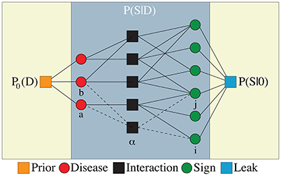
Figure 1. The interaction graph of disease variables (left circles) and sign variables (right circles) related by M_a = 3 one-disease and M_ab = 2 two-disease interaction factors (middle squares) in addition to interactions induced by the leak probability (right square) and the prior probability of diseases (left square). An interaction factor α = a, ab is connected to k_α signs and l_α diseases.

To obtain the model parameters ($K_i^0,K_i^{a,ab}$, and $K_{ij}^{a,ab}$), we start from the conditional marginals P_true(S_i|nodisease). This information is sufficient to determine the couplings $K_i^0$ from the following consistency equations:

$\begin{array}{ll}{P}_{true}(S_i|\text{nodisease})={\displaystyle \sum _{\{S_j:j\ne i\}}}P(\text{S}|\text{D}=0)\forall i.& (11)\end{array}$

If we have P_true(S_i, S_j|onlyD_a), then in principle we can find $K_i^a$ and $K_{ij}^a$ from similar consistency equations, assuming that we already know the $K_i^0$. Note that P(S_i, S_j|onlyD_a) is different from P(S_i, S_j|D_a), which is conditioned only on the value of disease a. In the same way, having the P_true(S_i, S_j|onlyD_a, D_b) allow us to find the couplings $K_i^{ab}$ and $K_{ij}^{ab}$, and so on. In general, the problem of finding the couplings from the above conditional probabilities is computationally expensive. However, there are many efficient approximate methods that enable us to find good estimations for the above couplings given the above conditional probabilities [35, 37–40, 42, 44]. The reader can find more details about the models in Supplementary Material (Section 1), where we provide a very simple learning algorithm, which is based on the Bethe approximation, for estimating the model parameters, given the above marginal probabilities.

3.2. Computing the Marginal Probabilities: An Approximate Inference Algorithm

Let us consider a simple benchmark model to check the performances of the above constructed models. As the benchmark, we take the true conditional probability

$\begin{array}{ll}{P}_{true}(\text{S}|\text{D})=\frac{1}{Z_{true}(\text{D})}{e}^{-H(\text{S},{\text{S}}^{*}(\text{D}))},& (12)\end{array}$

where S*(D) gives the most probable symptoms of hypothesis D. We choose these symptoms randomly and uniformly from the space of sign variables. That is, the value of each sign $S_i^{*}(\text{D})$ (for i = 1, …, N_S) is chosen to be positive or negative with equal probability 1/2. Moreover, $H(\text{S},{\text{S}}^{*}(\text{D}))\equiv \sum _{i=1}^{N_S}{(S_i-S_i^{*}(\text{D}))}^2/4$ is the Hamming distance (number of different signs) of the two sign configurations. Note that there is no sign-sign interaction in the above true model. Therefore, given the true conditional marginals, we can exactly compute the model parameters, as described in Supplementary Material (Section 1).

For small numbers of sign/disease variables, we can use an exhaustive inference algorithm to compute the exact marginal probabilities. Figure 2 displays the root-mean-square (RMS) errors in the disease probabilities (compared with the true values), and the accuracy of the model predictions for the present diseases identified by the most probable diseases. Here we consider the cases in which only one or two diseases are present in the selected disease patterns. We compare the results that are obtained by the one-disease-one-sign (D1S1) and two-disease-one-sign (D2S1) models, with those that are obtained by the Bayes' rule assuming the conditional independence of the signs and causal independence of the diseases as computed in Shwe et al. [21]. The statistical information we need to obtain the model parameters and compute the disease probabilities are extracted from the exponential true model. As the figure shows, the D2S1 model results in much smaller errors and better predictions when two diseases are responsible for the observed signs. This computation is intended to exhibit the high impact of two-disease interactions on the behavior of the marginal probabilities. We will soon see that these large effects of interactions can indeed play a constructive role also in the process of diagnosis.

FIGURE 2

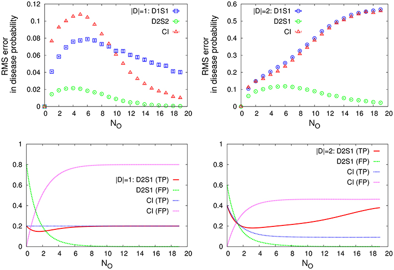
Figure 2. (Top) The RMS error in the disease probability and (Bottom) the accuracy of the disease predictions, true positive (TP) and false positive (FP), for cases in which only one (|D| = 1) or two diseases (|D| = 2) are present in the disease hypothesis. We compare the results obtained by the D1S1 and D2S1 models with the (CI) results obtained by the Bayes' rule assuming the conditional independence of the signs and causal independence of the diseases. The model parameters are obtained from the conditional marginals of the exponential true model. Here N_D = 5, N_S = 20, and N_O is the number of observed signs with the true values. The prior probabities are chosen such that N_DP₀(D_a = 1) = |D|. The data are results of averaging over 1,000 independent realizations of the true model and the true disease pattern.

To infer the marginal probabilities of the models for larger number of sign/disease variables, we resort to the Bethe approximation and the Belief-Propagation algorithm [33, 46]. First, we suggest an approximate expression for the normalization function Z(D), which appears in the denominator of the conditional probability distribution P(S|D). In words, we consider this non-negative function of the diseases to be a probability measure, and we approximate this measure by a factorized probability distribution, using its one- and two-variable marginal probabilities (see Supplementary Material, Section 2). This approximation enables us to employ an efficient message-passing algorithm such as belief propagation for computing statistical properties of the above models. As mentioned before, we shall assume that the prior probability P₀(D) can also be written in an appropriate factorized form. The quality of our approximations depends very much on the structure of the interaction factors and the strengths of the associated couplings in the models. The Bethe approximation is exact for interaction graphs that have a tree structure. This approximation is also expected to work very well in sparsely connected graphs, in which the number of interaction factors (M_a, M_ab) and the number of signs associated with an interaction factor (k_a, k_ab) are small compared with the total number of sign variables. In Supplementary Material (Section 2) we display the relative errors in the marginal signs/diseases probabilities that were obtained by the above approximate algorithm. The time complexity of our approximate inference algorithm grows linearly with the number of interaction factors and exponentially with the number of variables that are involved in such interactions; with N_D = 500, N_S = 5, 000, M_a = 500, M_ab = 1, 000, k_a = 10, k_ab = 5, the algorithm takes ~1 min of CPU time on a standard PC to compute the local marginals. We recall that the INTERNIST algorithm works with 534 diseases and ~4,040 signs (or manifestations), with 40,740 directed links that connect the diseases to the signs [21].

3.3. Optimization of the Diagnosis Process: A Stochastic Optimization Problem

Suppose that we know the results of N_O observations (medical tests), and we choose another unobserved sign j ∈ U for observation. To measure the performance of our decision, we may compute deviation of the disease probabilities from the neutral values (or “disease polarization”) after the observation:

$\begin{array}{ll}DP(j)\equiv {\left(\frac{1}{N_D}{\displaystyle \sum _a}{\left(P(D_a=1)-\frac{1}{2}\right)}^2\right)}^{1/2}.& (13)\end{array}$

One can also add other measures such as the cost of observation to the above function.

In a two-stage decision problem, we choose an unobserved sign for observation, with the aim of maximizing the averaged objective function ${E}(j)\equiv {\langle DP(j)\rangle }_O$. Note that before doing any real observation, we have access only to the probability of the outcomes P(S_j); the actual or true value of an unobserved sign becomes clear only after the observation. That is why here we are taking the average over the possible outcomes, which is denoted by 〈·〉_O. One can repeat the two-stage problem for T times to obtain a sequence of T observations: each time an optimal sign is chosen for observation followed by a real observation, which reveals the true value of the observed sign.

In a multistage version of the problem, we want to find an optimal sequence of decisions O_T = {j₁, …, j_T}, which maximizes the following objective functional of the observed signs: ${E}\left[O_T\right]\equiv \sum _{t=1}^T{\langle DP(j_t)\rangle }_O$. Here, at each step, the “observed” sign takes a value that is sampled from the associated marginal probability P(S_j). This probability depends on the model which we are working with. Note that here we are interested in finding an optimal sequence of observations at the beginning of the process before doing any real observation. In other words, in such a multistage problem, we are doing an “extrapolation” or “simulation” of the observation process without performing any real observation. In practice, however, we may fix the sequence of observations by a decimation algorithm: i.e., we repeat the multistage problem for T times, where each time we observe the first sign suggested by the output sequence, and reduce the number of to-be-observed signs by one.

In the following, we consider only simple approximations of the multistage problem; first we reduce the difficult multistage problem to simpler two-stage problems. More precisely, at each time step, we choose an unobserved sign j_t, which results to the largest disease polarization 〈DP(j_t)〉_O, for observation (greedy strategy). Then, we consider two cases: (I) we perform a real observation to reveal the true value of the suggested sign for observation, (II) we treat the suggested sign variable for observation as a stochastic variable with values that are sampled from the associated marginal probability.

Let us start from the case in which we observe the true values of the signs chosen for observation. Once again, we take the exponential benchmark model given by Equation (12) as the true model. We use the conditional marginals extracted from this true model to construct the simple one-disease-one-sign (D1S1) and two-disease-one-sign (D2S1) models. Suppose that we are given a disease hypothesis D and the associated symptoms S*(D). We start from a few randomly chosen observed signs from the set of symptoms. Then, at each time step t, we compute the inferred sign probabilities P(S_j), and use the greedy strategy to choose an unobserved sign for observation. The observed sign at each step takes the true value given by S*(D). To see how much the disease probabilities obtained from the models are correlated with the true (or maximum likelihood) hypothesis D, we compute the following overlap function (or “disease likelihood”):

$\begin{array}{ll}DL(t)\equiv \frac{1}{N_D}{\displaystyle \sum _a}(2D_a-1)\left(P(D_a=1)-\frac{1}{2}\right).& (14)\end{array}$

Besides the magnitude, our decisions also affect the way that the above quantity behaves with the number of observations.

In Figure 3 we see how the above overlap function, DL(t), behaves for cases in which only one or two diseases are present in D (see also Supplementary Material, Section 3). For comparison, we also show the results obtained by a random strategy, where an unobserved sign is chosen for observation randomly and uniformly from the subset of unobserved signs. The number of sign/disease variables here is small enough to allow for an exact computation of all the marginal probabilities. It is seen that both the D1S1 and D2S1 models work very well when only one disease is present and all the other diseases are absent. The D1S1 model already fails when two diseases are present in the hypothesis, whereas the other model can still find the right diseases. However, we observe that even the D2S1 model gets confused when there are more than two diseases in the hypothesis; in such cases, we would need to consider more sophisticated models with interactions involving more than two diseases. Moreover, we observe that the difference in the performances of the greedy and random strategies decreases as the number of involved diseases increases. In Supplementary Material (Section 3), we observe similar behaviors for a more complex benchmark model $P_{true}(\text{S}|\text{D})\propto 1/(1+H(\text{S},{\text{S}}^{*}(\text{D})))$, including also the sign-sign interactions.

FIGURE 3

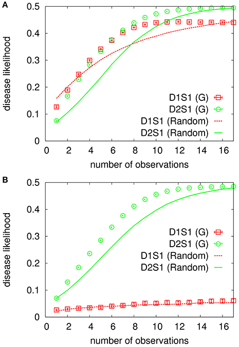
Figure 3. Overlap of the inferred disease marginals with the true hypothesis for the exponential benchmark model. The data are for the cases in which only one (A) or two (B) diseases are present. The model parameters are obtained from the conditional marginals of the true model. There are N_D = 5 diseases, N_S = 20 signs, and the algorithm starts with N_O = 3 observed signs for a randomly selected hypothesis D. An unobserved sign is chosen for observation by the greedy (G) or random strategy using the inferred probabilities, and the observed sign takes the true value given by S*(D). The data are results of averaging over 1000 independent realizations of the true model and the observation process.

Next, we consider the case of simulating the diagnosis process without doing any real observation. Here, we assume that an observed sign takes a value which is sampled from the associated marginal probability P(S_j) at that time step. For comparison with the greedy strategy, we also introduce two other strategies for choosing an unobserved sign for observation. A naive strategy is to choose the most positive (MP) sign $j_{max}=arg\underset{j}{max}\left\{P(S_j=+1)\right\}$ for observation (MP strategy); j_max is the sign with the maximum probability of being positive. In the early stages of the diagnosis, this probability is probably close to zero for most of the signs. So, it makes sense to choose the most positive sign for observation to obtain more information about the diseases. A more complicated strategy works by first computing the conditional probabilities P(S_j|D_ML) for the maximum likelihood hypothesis D_ML, and then selecting the most positive sign for observation (MPD strategy).

To have a more general comparison of the constructed models, in the following, we assume that the model parameters ($K_i^{a,ab}$, and $K_{ij}^{a,ab}$) are iid random numbers uniformly distributed in an appropriate interval of real numbers. The leaky couplings are set to $K_i^0=-1$, which correspond to small sign probabilities P(S_i = 1|nodisease) ≃ 0.1. We assume that all the possible one-disease and two-disease interaction factors are present in the models. Moreover, inside each factor we have all the possible two-sign interactions in addition to the local sign fields. As before, the prior disease probabilities P₀(D_a) are uniform probability distributions. Figure 4 shows the performances for different models and strategies with a small number of sign/disease variables. Here, the “disease likelihood” gives the overlap of the disease probabilities with the maximum likelihood hypothesis D_ML of the models. Moreover, all the quantities are computed exactly. We see that in this case the average performance of the greedy strategy is close to that of the MPD strategy at the beginning of the process. For larger number of observations, the greedy performance degrades and approaches that of the MP strategy.

FIGURE 4

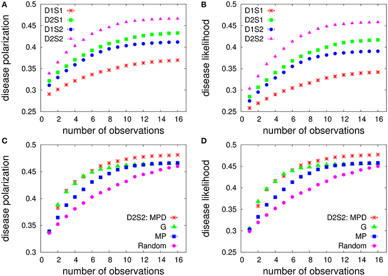
Figure 4. Diagnostic performance of the models vs. the number of observations for a small number of sign/disease variables. (Top) The exact disease-polarization (A) and disease-likelihood (B) obtained by the MP strategy in the one-disease-one-sign (D1S1), two-disease-one-sign (D2S1), one-disease-two-sign (D1S2), and two-disease-two-sign (D2S2) models. There are N_D = 5 diseases, N_S = 20 signs, and the algorithm starts with N_O = 4 observed signs with positive values. The couplings in the interaction factors are iid random numbers distributed uniformly in the specified intervals: $K_i^0=-1,K_i^{a,ab}\in (-1,+1),K_{i,j}^{a,ab}\in (-1,+1)/\sqrt{N_S}$. (Bottom) Comparing the exact polarization (C) and likelihood (D) of the diseases obtained by the MP, greedy (G), MPD, and random strategies, for the D2S2 model. The data are results of averaging over 1,000 independent realizations of the model parameters.

The models with disease-disease and sign-sign interactions exhibit larger polarizations of the disease probabilities and larger overlaps of the disease probabilities with the maximum-likelihood hypothesis (see also Supplementary Material, Section 3); we find that already the D2S1 model works considerably better than the D1S1 model for disease-disease interactions of relative strengths $|K_i^{ab}/K_i^a|\simeq 0.3$. A larger polarization means that we need a smaller number of observations (medical tests) to obtain more definitive disease probabilities. A larger disease likelihood, here means that we are following the direction that is suggested by the most likely diseases. In this sense, it appears that the two-sign/disease interactions could be very helpful in the early stages of the diagnosis.

We checked that the above picture also holds if we start with different numbers of observed signs, and if we double the magnitude of all the couplings. Similar behaviors are observed also for larger problem sizes (see Supplementary Material, Section 3). However, we see that for strongly interacting models with much larger higher-order interactions, e.g., $K_i^0=-1$, and $K_i^{a,ab}\in (-2,+2),K_{ij}^{a,ab}\in (-2,+2)/\sqrt{N_S}$, the MP strategy gets closer to the random strategy. The fact that the MP strategy does not work well in this strongly correlated regime was indeed expected. Here, the greedy strategy is working better than the MPD strategy, and both are still performing better than the random strategy.

4. Discussions

In summary, we showed that considering the sign-sign and disease-disease interactions can significantly change the statistical importance of the signs and diseases. More importantly, we found that these higher-order correlations could be very helpful in the process of diagnosis, especially in the early stages of the diagnosis. The results in Figures 3, 4 (and similar figures in Supplementary Material) also indicate the significance and relevance of optimization of the diagnosis procedure, where a good strategy could considerably increase the polarization and likelihood of the diseases compared to the random strategy. In addition, we devised an approximate inference algorithm with a time complexity that grows linearly with the number of interaction factors connecting the diseases to the signs, and exponentially with the maximum number of signs that are associated with such interaction factors. For clarity, in this work, we considered only algorithms of minimal structure and complexity. It would be straightforward to employ more accurate learning and inference algorithms in constructing the models and inferring the statistical information from the models. The challenge is, of course, to go beyond the heuristic and greedy algorithms that we used to study the multistage stochastic optimization problem of deciding on the relevance and order of the medical observations.

In this study, we considered very simple structures for the prior probability of the diseases P₀(D) and the leak probability of the signs P(S|nodisease). Obviously, depending on the available statistical data, we can obtain more reliable models also for these probability distributions. Alternatively, we could employ the maximum entropy principle to construct directly the joint probability distribution of the sign and disease variables using the joint marginal probabilities P(S_i, S_j; D_a, D_b). Note that, in practice, it is easier to obtain this type of information than the stronger conditional probabilities P(S_i, S_j|onlyD_a) and P(S_i, S_j|onlyD_a, D_b). However, these measures are easier to model (or estimated by experts), in the absence of enough observational data, because they present the sole effects of single (or few) diseases.

The emphasize, in this study, was more on the diagnostic performances of the models than on the statistical significance of the selected models for a given set of clinical data. In other words, we assumed that we have access to the true marginal probabilities P_true(S_i|nodisease), P_true(S_i, S_j|onlyD_a) and P_true(S_i, S_j|onlyD_a, D_b) of the true probabilistic model describing the statistical behavior of the sign and disease variables. Then, the model structure is determined by the maximum entropy principle depending on the nature of the provided local probability marginals. A more accurate treatment of the model selection, for a finite collection of data, accounts also the complexity of the models to avoid the over-fitting of the data. Here, it is the statistical quality of the available data that determines the best model which results to smaller prediction errors. We note that including the sign-sign and disease-disease interactions in the models is indeed more natural than ignoring such correlations. The results obtained in this study in fact highlight the necessity of collecting the relevant clinical data to benefit from such informative correlations. Finally, to take into account the role of noises in the model parameters, one should take the average of the objective function over the probability distribution of the parameters, which is provided by the likelihood of the model parameters.

Our proposed framework can be adapted to address assignment problems in cell biology, immunology, and evolutionary biology [60–63]. In contrast to clinical problems, here data availability might be less of a problem in near future. Advances in genomics, transcriptomics, proteomics and metabolomics promise high resolution molecular characterization of cells. Intensive research has also been directed toward live single cell analysis which allows characterization of pathways from an initial state to a final state [64]. Our approach can be used to do early assignments and thus not only provides accuracy but also an improved sensitivity for diagnostics at the cellular level.

5. Materials and Methods

To construct the models we need the statistical information that connect the sign and disease variables P_true(S_i|nodisease), P_true(S_i|onlyD_a), …. In the absence of the sign-sign interactions, we can easily obtain the model parameters by the following expressions,

$\begin{array}{ll}{K}_i^0=\frac{1}{2}ln\left(\frac{P_{true}(S_i=+1|\text{nodisease})}{P_{true}(S_i=-1|\text{nodisease})}\right),& (15)\end{array}$

$\begin{array}{ll}{K}_i^a=\frac{1}{2}ln\left(\frac{P_{true}(S_i=+1|\text{only}{D}_a)}{P_{true}(S_i=-1|\text{only}{D}_a)}\right)-K_i^0,& (16)\end{array}$

$\begin{array}{ll}{K}_i^{ab}=\frac{1}{2}ln\left(\frac{P_{true}(S_i=+1|\text{only}{D}_a,D_b)}{P_{true}(S_i=-1|\text{only}{D}_a,D_b)}\right)-K_i^0-K_i^a-K_i^b.& (17)\end{array}$

The partition function here reads as follows,

$\begin{array}{ll}Z(\text{D})={\displaystyle \prod _i}\left(2cosh(K_i^0+{\displaystyle \sum _a}{D}_a{K}_i^a+{\displaystyle \sum _{a<b}}{D}_a{D}_b{K}_i^{ab})\right).& (18)\end{array}$

In general, however, we have to use approximation methods to obtain the parameters and the partition function (Supplementary Material, Sections 1, 2). In particular, the latter is a nonnegative function and can be considered as a probability measure over the disease variables. Then, within the Bethe approximation, the partition function can be approximated by

$\begin{array}{ll}Z(\text{D})\propto {\displaystyle \prod _a}{\mu }_a(D_a){\displaystyle \prod _{\alpha }}\left(\frac{{\mu }_{ab}(D_a,D_b)}{{\mu }_a(D_a){\mu }_b(D_b)}\right).& (19)\end{array}$

where μ_a(D_a) and μ_ab(D_a, D_b) are the associated marginal probabilities.

The above factorization allows us to compute the marginal sign and disease probabilities by a message-passing algorithm (Supplementary Material, Section 2),

$\begin{array}{ll}P(S_i)\propto e^{K_i^0{S}_i}{\displaystyle \prod _{\alpha \in \partial i}}{\tilde{\Psi }}_{\alpha \to i}(S_i),& (20)\end{array}$

$\begin{array}{ll}P(D_a)\propto P_0(D_a){\displaystyle \prod _{\alpha \in \partial a}}{\tilde{\Psi }}_{\alpha \to a}(D_a).& (21)\end{array}$

Here ∂i and ∂a stand for the subset of interaction factors α = a, ab that are connected to sign i and disease a, respectively. Similarly, we use ∂_Sα and ∂_Dα for the subset of sign and disease variables which appear in interaction factor α. The cavity messages ${\tilde{\Psi }}_{\alpha \to i}(S_i)$ and ${\tilde{\Psi }}_{\alpha \to a}(D_a)$ satisfy the Belief Propagation Equations [33],

$\begin{array}{l}{\tilde{\Psi }}_{\alpha \to i}(S_i)\propto {\displaystyle \sum _{\{D_a:a\in {\partial }_D\alpha \}}}{\displaystyle \sum _{\{S_j:j\in {\partial }_S\alpha \backslash i\}}}{\tilde{\varphi }}_{\alpha }({\text{S}}^{\alpha }|{\text{D}}^{\alpha })\\ {\displaystyle \prod _{a\in {\partial }_D\alpha }}{\nu }_{a\to \alpha }(D_a){\displaystyle \prod _{j\in {\partial }_S\alpha \backslash i}}{\nu }_{j\to \alpha }(S_j),& (22)\end{array}$

$\begin{array}{l}{\tilde{\Psi }}_{\alpha \to a}(D_a)\propto {\displaystyle \sum _{\{D_b:b\in {\partial }_D\alpha \backslash a\}}}{\displaystyle \sum _{\{S_j:j\in {\partial }_S\alpha \}}}{\tilde{\varphi }}_{\alpha }({\text{S}}^{\alpha }|{\text{D}}^{\alpha })\\ {\displaystyle \prod _{b\in {\partial }_D\alpha \backslash a}}{\nu }_{b\to \alpha }(D_b){\displaystyle \prod _{j\in {\partial }_S\alpha }}{\nu }_{j\to \alpha }(S_j).& (23)\end{array}$

and

$\begin{array}{ll}{\nu }_{i\to \alpha }(S_i)\propto e^{K_i^0{S}_i}{\displaystyle \prod _{\beta \in \partial i\ne \alpha }}{\tilde{\Psi }}_{\beta \to i}(S_i),& (24)\end{array}$

$\begin{array}{ll}{\nu }_{a\to \alpha }(D_a)\propto P_0(D_a){\displaystyle \prod _{\beta \in \partial a\ne \alpha }}{\tilde{\Psi }}_{\beta \to a}(D_a).& (25)\end{array}$

The rescaled disease factors are given by

$\begin{array}{ll}{\tilde{\varphi }}_a\equiv \frac{{\varphi }_a}{{\mu }_a(D_a)},{\tilde{\varphi }}_{ab}\equiv {\mu }_a(D_a){\mu }_b(D_b)\frac{{\varphi }_{ab}}{{\mu }_{ab}(D_a,D_b)}.& (26)\end{array}$

These equations are solved by iteration; we start from random initial messages, and update the cavity marginals according to the above equations until the algorithm converges.

At each step of the diagnostic process we need the marginal sign and disease probabilities, which can be estimated by the above approximation algorithm. For sparse interaction graphs, the computation time of this algorithm grows linearly with the number of interaction factors M_a, M_ab ∝ N_D. Then, the time complexity of the greedy strategy is proportional to TN_SN_D, where T is the number of observations. In the MP strategy, we do not need to check every unobserved sign to see what happens after the observation, therefore the computation time is ∝ TN_D. This is true also for the MPD strategy, if we use the most probable disease values instead of the maximum-likelihood values D_ML.

Author Contributions

AM conceived the project. AR acquired the data and performed the simulations. AR and AM designed the work, analyzed and interpreted the data, wrote the paper, and approved the published version.

Conflict of Interest Statement

The authors declare that the research was conducted in the absence of any commercial or financial relationships that could be construed as a potential conflict of interest.

Supplementary Material

The Supplementary Material for this article can be found online at: https://www.frontiersin.org/article/10.3389/fphy.2017.00032/full#supplementary-material

References

1. DuPage M, Bluestone JA. Harnessing the plasticity of CD4+ T cells to treat immune-mediated disease. Nat Rev Immunol. (2016) 16:149–63. doi: 10.1038/nri.2015.18

PubMed Abstract | CrossRef Full Text | Google Scholar

2. Holzel M, Bovier A, Tuting T. Plasticity of tumour and immune cells: a source of heterogeneity and a cause for therapy resistance? Nat Rev Cancer (2016) 13:365–76. doi: 10.1038/nrc3498

PubMed Abstract | CrossRef Full Text

3. Saeys Y, Van Gassen, S, Lambrecht BN. Computational flow cytometry: helping to make sense of high-dimensional immunology data. Nat Rev Immunol. (2016) 16:449–62. doi: 10.1038/nri.2016.56

PubMed Abstract | CrossRef Full Text | Google Scholar

4. Patti GJ, Yanes O, Siuzdak G. Metabolomics: the apogee of the omics, trilogy. Nat Rev Mol Cell Biol. (2012) 13:263–9. doi: 10.1038/nrm3314

PubMed Abstract | CrossRef Full Text

5. Kasper D, Fauci F, Hauser S, Longo D, Jameson J, Loscalzo J. Harrison's Principles of Internal Medicine, 19 Edn. New York, NY: McGraw-Hill Education (2015).

6. Papadakis M, McPhee SJ, Rabow MW. Current Medical Diagnosis and Treatment, 55 Edn. LANGE CURRENT Series. New York, NY: McGraw-Hill Education (2016).

7. Lerner AJ. Diagnostic Criteria in Neurology. Totowa, NJ: Humana Press (2006).

Google Scholar

8. Coggon D, Martyn C, Palmer KT, Evanoff B. Assessing case definitions in the absence of a diagnostic gold standard. Int J Epidemiol. (2005) 34:949–52. doi: 10.1093/ije/dyi012

PubMed Abstract | CrossRef Full Text | Google Scholar

9. Greenes R. Clinical Decision Support, The Road to Broad Adoption. 2nd Edn. Cambridge, MA: Academic Press (2014).

Google Scholar

10. Miller RA, Pople HE Jr., Myers JD. Internist-I, an experimental computer-based diagnostic consultant for general internal medicine. N Engl J Med. (1982) 307:468–76. doi: 10.1056/NEJM198208193070803

PubMed Abstract | CrossRef Full Text | Google Scholar

11. Heckerman DE. Formalizing Heuristic Methods for Reasoning with Uncertainty. Technical Report KSL-88-07, Stanford, CA: Medical Computer Science Group, Section on Medical Informatics, Stanford University (1987).

12. Horvitz EJ, Breese JS, Henrion M. Decision theory in expert systems and artificial intelligence. Int J Approximate Reason. (1988) 2:247–302. doi: 10.1016/0888-613X(88)90120-X

CrossRef Full Text | Google Scholar

13. Shortliffe EH. The adolescence of AI in medicine: will the field come of age in the 90's? Artif Intell Med. (1993) 5:93–106. doi: 10.1016/0933-3657(93)90011-Q

PubMed Abstract | CrossRef Full Text | Google Scholar

14. Adams JB. A probability model of medical reasoning and the MYCIN model. Math Biosci. (1976) 32:177–86. doi: 10.1016/0025-5564(76)90064-X

CrossRef Full Text | Google Scholar

15. Buchanan BG, Shortliffe EH (Eds.). Rule-based Expert Systems, Vol. 3. Reading, MA: Addison-Wesley (1984).

Google Scholar

16. Miller R, Masarie FE, Myers JD. Quick medical reference (QMR) for diagnostic assistance. Comput Med Pract. (1985) 3:34–48.

PubMed Abstract | Google Scholar

17. Barnett GO, Cimino JJ, Hupp JA, Hoffer E. P. DXplain: an evolving diagnostic decision-support system. JAMA (1987) 258:67–74. doi: 10.1001/jama.1987.03400010071030

PubMed Abstract | CrossRef Full Text | Google Scholar

18. Spielgelharter DJ. Probabilistic expert systems in medicine. Stat Sci. (1987) 2:3–44. doi: 10.1214/ss/1177013426

CrossRef Full Text

19. Bankowitz RA, McNeil MA, Challinor SM, Parker RC, Kapoor WN, Miller RA. A computer-assisted medical diagnostic consultation service: implementation and prospective evaluation of a prototype. Ann Int Med. (1989) 110:824–32. doi: 10.7326/0003-4819-110-10-824

PubMed Abstract | CrossRef Full Text | Google Scholar

20. Heckerman D. A tractable inference algorithm for diagnosing multiple diseases. In Henrion M, Shachter R, Kanal LN, Lemmer JF, editors. Machine Intelligence and Pattern Recognition: Uncertainty in artificial Intelligence 5. Amsterdam North Holland Publ. Comp. (1990). p. 163–72.

Google Scholar

21. Shwe MA, Middleton B, Heckerman DE, Henrion M, Horvitz EJ, Lehmann HP, et al. Probabilistic diagnosis using a reformulation of the INTERNIST-1/QMR knowledge base. Methods Inform Med. (1991) 30:241–55.

Google Scholar

22. Heckerman DE, Shortliffe EH. From certainty factors to belief networks. Artif Intell Med. (1992) 4:35–52. doi: 10.1016/0933-3657(92)90036-O

CrossRef Full Text | Google Scholar

23. Nikovski D. Constructing Bayesian networks for medical diagnosis from incomplete and partially correct statistics. IEEE Trans Knowl Data Eng. (2000) 12:509–16. doi: 10.1109/69.868904

CrossRef Full Text | Google Scholar

24. Przulj N, Malod-Dognin N. Network analytics in the age of big data. Science (2016) 353:123–4. doi: 10.1126/science.aah3449

PubMed Abstract | CrossRef Full Text | Google Scholar

25. Hamaneh MB, Yu YK. DeCoaD: determining correlations among diseases using protein interaction networks. BMC Res Notes (2015) 8:226. doi: 10.1186/s13104-015-1211-z

PubMed Abstract | CrossRef Full Text | Google Scholar

26. Zitnik M, Janjic V, Larminie C, Zupan B, Natasa Przuljb N. Discovering disease-disease associations by fusing systems-level molecular data. Sci Rep. (2013) 3:3202. doi: 10.1038/srep03202

PubMed Abstract | CrossRef Full Text | Google Scholar

27. Liu W, Wu A, Pellegrini M, Wanga X. Integrative analysis of human protein, function and disease networks. Sci Rep. (2015) 5:14344. doi: 10.1038/srep14344

PubMed Abstract | CrossRef Full Text | Google Scholar

28. Suratanee A, Plaimas K. DDA: a novel network-based scoring method to identify disease-disease associations. Bioinform Biol Insights (2015) 9:175–86. doi: 10.4137/BBI.S35237

PubMed Abstract | CrossRef Full Text | Google Scholar

29. Gustafsson M, Nestor CE, Zhang H, Barabasi AL, Baranzini S, Brunak S, et al. Modules, networks and systems medicine for understanding disease and aiding diagnosis. Genome Med. (2014) 6:82. doi: 10.1186/s13073-014-0082-6

PubMed Abstract | CrossRef Full Text | Google Scholar

30. Liu CC, Tseng YT, Li W, Wu CY, Mayzus I, Rzhetsky A, et al. DiseaseConnect: a comprehensive web server for mechanism-based disease-disease connections. Nucl Acids Res. (2015) 42:W137–46. doi: 10.1093/nar/gku412

PubMed Abstract | CrossRef Full Text | Google Scholar

31. Sun K, Goncalves JP, Larminie C, Przulj N. Predicting disease associations via biological network analysis. BMC Bioinformatics (2014) 15:304. doi: 10.1186/1471-2105-15-304

PubMed Abstract | CrossRef Full Text | Google Scholar

32. Jordan MI. Graphical models. Stat Sci. (2004) 19:140–55. doi: 10.1214/088342304000000026

CrossRef Full Text | Google Scholar

33. Mezard M, Montanari A. Information, Physics, and Computation. Oxford: Oxford University Press (2009).

Google Scholar

34. Altarelli F, Braunstein A, Ramezanpour A, Zecchina R. Stochastic matching problem. Phys Rev. Lett. (2011) 106:190601. doi: 10.1103/PhysRevLett.106.190601

PubMed Abstract | CrossRef Full Text | Google Scholar

35. Ricci-Tersenghi F. The Bethe approximation for solving the inverse Ising problem: a comparison with other inference methods. J Stat Mech Theory Exp. (2012) 2012:P08015. doi: 10.1088/1742-5468/2012/08/P08015

CrossRef Full Text | Google Scholar

36. Edwin T. Jaynes. Probability Theory: the Logic of Science. Cambridge: Cambridge University Press (2003).

37. Kappen HJ, Rodriguez FB. Efficient learning in Boltzmann machines using linear response theory. Neural Comput. (1998) 10:1137–56. doi: 10.1162/089976698300017386

CrossRef Full Text | Google Scholar

38. Tanaka T. Mean-field theory of Boltzmann machine learning. Phys Rev E (1998) 58:2302. doi: 10.1103/PhysRevE.58.2302

CrossRef Full Text | Google Scholar

39. Schneidman E, Berry MJ, Segev R, Bialek W. Weak pairwise correlations imply strongly correlated network states in a neural population. Nature (2006) 440:1007–12. doi: 10.1038/nature04701

PubMed Abstract | CrossRef Full Text | Google Scholar

40. Cocco S, Leibler S, Monasson R. Neuronal couplings between retinal ganglion cells inferred by efficient inverse statistical physics methods. Proc Natl Acad Sci USA (2009) 106:14058-62. doi: 10.1073/pnas.0906705106

PubMed Abstract | CrossRef Full Text | Google Scholar

41. Weigt M, White RA, Szurmant H, Hoch JA, Hwa T. Identification of direct residue contacts in protein-protein interaction by message passing. Proc Natl Acad Sci USA (2009) 106:67–72. doi: 10.1073/pnas.0805923106

PubMed Abstract | CrossRef Full Text | Google Scholar

42. Roudi Y, Aurell E, Hertz JA. Statistical physics of pairwise probability models. Front Comput Neurosci. (2009) 3:22. doi: 10.3389/neuro.10.022.2009

PubMed Abstract | CrossRef Full Text | Google Scholar

43. Bailly-Bechet M, Braunstein A, Pagnani A, Weigt M, Zecchina R. Inference of sparse combinatorial-control networks from gene-expression data: a message passing approach. BMC Bioinformatics (2010) 11:355. doi: 10.1186/1471-2105-11-355

PubMed Abstract | CrossRef Full Text | Google Scholar

44. Nguyen HC, Berg J. Mean-field theory for the inverse Ising problem at low temperatures. Phys Rev Lett. (2012) 109:050602. doi: 10.1103/PhysRevLett.109.050602

PubMed Abstract | CrossRef Full Text | Google Scholar

45. Pearl J. Probabilistic Reasoning in Intelligent Systems: Networks of Plausible Inference. Burlington, MA: Morgan Kaufmann (2014).

Google Scholar

46. Kschischang FR, Frey BJ, Loeliger HA. Factor graphs and the sum-product algorithm. IEEE Trans Inform Theory (2001) 47:498–519. doi: 10.1109/18.910572

CrossRef Full Text | Google Scholar

47. Mézard M, Parisi G, Zecchina R. Analytic and algorithmic solution of random satisfiability problems. Science (2002) 297:812–5. doi: 10.1126/science.1073287

PubMed Abstract | CrossRef Full Text

48. Yedidia JS, Freeman WT, Weiss Y. Understanding belief propagation and its generalizations. Explor Artif Intell New Millennium (2003) 8:236–9. Available online at: http://www.cse.iitd.ac.in/~mittal/read_papers/bp/TR2001-22.pdf

Google Scholar

49. Birge JR, Louveaux F. Introduction to Stochastic Programming. Berlin: Springer Science & Business Media (2011).

Google Scholar

50. Kleywegt AJ, Shapiro A, Homem-de-Mello T. The sample average approximation method for stochastic discrete optimization. SIAM J Optim. (2002) 12:479–502. doi: 10.1137/S1052623499363220

CrossRef Full Text | Google Scholar

51. Heyman DP, Sobel MJ. Stochastic Models in Operations Research: Stochastic Optimization, Vol. 2. North Chelmsford, MA: Courier Corporation (2003).

Google Scholar

52. Garey MR, Johnson DS. Computers and Intractability: A Guide to the Theory of NP-Completeness. Dallas, TX: W. H. Freeman (1979).

Google Scholar

53. Cooper GF. The computational complexity of probabilistic inference using Bayesian belief networks. Artif Intell. (1990) 42:393–405. doi: 10.1016/0004-3702(90)90060-D

CrossRef Full Text | Google Scholar

54. Henrion M. Towards efficient probabilistic diagnosis in multiply connected belief networks. In: Oliver RM, Smith JQ, editors. Influence Diagrams, Belief Nets and Decision Analysis. Chichester: Wiley (1990). p. 385–407.

55. Heckerman D, Geiger D, Chickering DM. Learning Bayesian networks: the combination of knowledge and statistical data. Mach Learn. (1995) 20:197–243. doi: 10.1007/BF00994016

CrossRef Full Text | Google Scholar

56. Chickering DM. Learning Bayesian networks is NP-complete. In: Learning From Data. New York, NY: Springer (1996). p. 121–30. doi: 10.1007/978-1-4612-2404-4_12

CrossRef Full Text | Google Scholar

57. Lezon TR, Banavar JR, Cieplak M, Maritan A, Fedoroff NV. Using the principle of entropy maximization to infer genetic interaction networks from gene expression patterns. Proc Natl Acad Sci USA (2006) 103:19033–8. doi: 10.1073/pnas.0609152103

PubMed Abstract | CrossRef Full Text | Google Scholar

58. Bialek W, Ranganathan R. Rediscovering the power of pairwise interactions. arXiv preprint arXiv:0712.4397 (2007).

Google Scholar

59. Banavar JR, Maritan A, Volkov I. Applications of the principle of maximum entropy: from physics to ecology. J Phys. (2010) 22:063101. doi: 10.1088/0953-8984/22/6/063101

PubMed Abstract | CrossRef Full Text | Google Scholar

60. Barabási AL, Oltvai ZA. Network biology: understanding the cell's functional organization. Nat Rev Genet. (2004) 5:101–13. doi: 10.1038/nrg1272

PubMed Abstract | CrossRef Full Text | Google Scholar

61. Kim M, Rai N, Zorraquino V, Tagkopoulos I. Multi-omics integration accurately predicts cellular state in unexplored conditions for Escherichia coli. Nat Commun. (2016) 7:13090. doi: 10.1038/ncomms13090

PubMed Abstract | CrossRef Full Text | Google Scholar

62. Ebrahim A, Brunk E, Tan J, O'Brien EJ, Kim D, Szubin R, et al. Multi-omic data integration enables discovery of hidden biological regularities. Nat Commun. (2016) 7:13091. doi: 10.1038/ncomms13091

PubMed Abstract | CrossRef Full Text | Google Scholar

63. Candia J, Maunu R, Driscoll M, Biancotto A, Dagur P, McCoy P, et al. From cellular characteristics to disease diagnosis: uncovering phenotypes with supercells. PLoS Comput Biol. (2013) 9:e1003215. doi: 10.1371/journal.pcbi.1003215

PubMed Abstract | CrossRef Full Text | Google Scholar

64. Spiller DJ, Wood CD, Rand DA, White MRH. Measurement of single-cell dynamics. Nature (2010) 465:736–45. doi: 10.1038/nature09232

PubMed Abstract | CrossRef Full Text | Google Scholar