Transitions from Trees to Cycles in Adaptive Flow Networks

1. Introduction

Network structures are found in all of our everyday life, ranging from social interactions over technological infrastructure to natural systems. Networks serve vital functions on microscopic to macroscopic length scales, ranging from proteins, DNA, cells, organs and organisms [1]. An important function of networks is to transport people, goods, metabolites, and information among other [2–7]. While in technology, transport networks are relatively rigid and yield limited adaptivity, biological transport networks are capable of ensuring robust flow and operate satisfactorily over a vast range of parameters to prevent operational failure even under extreme conditions.

An example for one of the most advanced transport networks is the mammalian vascular network. Every second, the vasculature is without interruptions serving regions of the brain despite ever changing neural activity [8] or changing demands in other tissue [9]. The mammalian vasculature, composed of bifurcations (nodes) and vessels (links), is highly adaptive because vessel diameters (weights) dynamically adjust to changes in flow properties such as pressure and shear stress via a variety of vessel response mechanisms [9]. Several biophysical models have investigated the response mechanism of single vessels [10–13]. Here, we aim at understanding how an adaptive flow network may respond on a global network level. Notably, the mammalian vasculature forms a complex network [14, 15] displaying both tree-like [16] and cyclic motifs [17] which also are found in the leaves of trees or in power grid networks [18].

Recent work investigated optimal topology of flow networks from the perspective of their energy efficiency, damage resilience, or cost of repair [19–23], features which may be argued to have evolved over long time scales. From the perspective of optimization theory, it is interesting to note that depending on the shape of the cost function, tree-like or cyclic structures may be more effective [24–27], leading to phase transitions between tree-like and cyclic structures. Moreover, cycles not only confer redundant structures and thus improve damage resilience (i.e., another cost function), but may also be more favorable in the presence of fluctuations [20, 28].

However, while research on adaptive (co-evolving) networks from the perspective of theoretical physics is under active development, the understanding of adaptive flow networks in particular remains relatively un(der)explored in the field of network theory [29]. Thus, we consider the dynamic stability of particular network configurations given that vessels may adapt their diameters slowly over relatively short time scales. Specifically, we wish to address the following questions: given a flow network with dynamically adapting weights, (i) what network configurations (weights) are dynamically stable, and (ii) if non-uniform flow (load) fluctuations are present in the network, how far do these fluctuations affect adaptation into network regions where fluctuations are absent? In other words, when spatially inhomogeneous load fluctuations are present, does the network partition into clusters exhibiting tree-like motifs and cycles?

We wish to establish a fundamental understanding of the possible dynamics and gain insights from the perspective of network theory, nonlinear dynamics and physics, rather than of specifically physiological aspects. Thus, to obtain answers to the above questions, we dispose of the mathematical intricacies inherent to solving biophysically detailed models. Instead of building on physiological models of blood vessel changes which occur via acute responses in tone or the slower remodeling of the vessel [10–13, 30–32], we defer to simple conceptual models of adaptive flow networks, based on basic physical principles, allowing for analytical tractability.

We assume that the network has one constant inlet (source) and many outlets (sinks) subject to load fluctuations. In the language of vascular physiology, we model a bifurcating arterial network where the only inlet is a feeding artery, bifurcating in a tree-structure to the terminal nodes interfacing via capillaries to the venous network. At this interface, changing supply demands constitute load fluctuations which are rapid compared to the adaptive network dynamics. A similar (though physiologically different) situation is seen in (real) trees, where the stem feeds the tree with water and nutrients at a more or less constant rate. In the leaves, so-called stoma evaporate the sap, and their periodic opening and closing correspond to fluctuating sinks [28, 33]. Inspired by these natural networks, we wish to address two questions: How strong do load fluctuations need to be so that cyclic shunts (loops)¹ emerge in the network that break the topology of a spanning tree? How far do these cyclic shunts reach into the tree toward the feeding vessel, so that a non-uniform network structure emerges, divided into two subgraphs, one tree-like and the other with cycles?

The article is organized as follows. In the next section, we introduce the model and simulations that we study. Sections 3 and 4 discuss the dynamics on simple network motifs (one source and one sink, and one source and two sinks, respectively). In section 5 we investigate the emergence of cyclic structures in a larger network with one constant source and many fluctuating loads, which we conclude in the Discussion in section 6.

2. Model

2.1. Network Structure

V denotes the set of nodes of the network with N = |V| < ∞ and A ⊆ N × N the set of edges. The edges are bidirectional, so (i, j) ∈ A implies (j, i) ∈ A. Each node is assigned a pressure p_i. The edge flow is f_ij > 0 from node i to j. Furthermore we assume that the network is resistive and linear, i.e., it is Ohmian with f_ij = C_ij(p_i − p_j), where an edge carries the property of a conductance between nodes i and j with C_ij = C_ji > 0 only if (i, j) ∈ A.

Here, we study the three kinds of wirings illustrated in Figure 1: (a) one source and one sink, (b) one source and two fluctuating sinks, (c) a tree-like network with height H allowing for cross-edges on every bifurcation/branching level, l = 0, …, H, leading to cyclic structure. A cycle is a connected subnetwork of m nodes such that each node has exactly two neighbors.

FIGURE 1

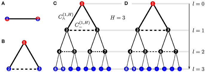
Figure 1. Network structures: (A) motif with 1 fluctuating source and 1 sink (2-node model), (B) motif with 1 constant source and 2 fluctuating sinks (3-node model), and “augmented trees” (C,D), i.e., tree-like structures with cross-edges (dashed horizontal edges) that connect only nodes in each minimal subtree, thus forming a “triangular tree” (C), or connect all nodes within one tree level l by a path as in (D). Thus, cross edges introduce cycles to the network. The constant source at the root and the fluctuating sinks in the leaves of the tree are shown in blue and red, respectively, and l denotes the branching level in the tree-like structure.

To model sources and sinks in the network, we include non-zero nodal flows h_i. Denote by S ⊂ V the set of sink nodes, |S| = n = 2^H. We define one source at the edge feeding the network, h₁ = 1, and n sinks with h_i(t) < 0 at all leaves of the tree-like structure (i.e., where capillaries connect to the vein network). For all other nodes, h_i = 0. Mass balance requires that $\sum _{k\in V}{h}_k(t)=0$ for all t ∈ ℝ.

2.2. Mass Conservation

Mass conservation demands that edge flows, f_ij from node i to adjacent nodes j, and nodal flows, h_i, match the local accumulation rate at node i, dV_i/dt, i.e.,

$\begin{array}{cc}\begin{array}{l}\rho \frac{d}{dt}{V}_i+{\displaystyle \sum _j{f}_{ij}}=h_i(t)\hfill \end{array}& (1)\end{array}$

where ρ is the fluid density and V_i is the vessel volume at node i. However, assuming that accumulation is nearly instantaneous or vessels are inelastic the nodal accumulation rate becomes negligible [15]. Mass balance then becomes Kirchhoff's first law stating that

$\begin{array}{cc}\begin{array}{l}{\displaystyle \sum _j{C}_{ij}}(p_i-p_j)=h_i,\hfill \end{array}& (2)\end{array}$

which is re-written in vector/matrix notation by defining the nodal flow h : = (h_i)_i∈V and the Kirchhoff matrix K = (_{Kij)i, j∈V} with $K_{ij}:=({\delta }_{ij}\sum _j{C}_{ij})-C_{ij}$,

$\begin{array}{cc}\begin{array}{l}K·p=h\hfill \end{array}& (3)\end{array}$

which is solved for p : = (pi)_i∈V.

2.3. Dynamically Adapting Conductances

To impose adaptive dynamics to the network, we postulate the generic ad-hoc law for the conductances:

$\begin{array}{cc}\begin{array}{l}\frac{d}{dt}{C}_{ij}={\alpha }_1{C}_{ij}{(p_j-p_i)}^2-{\alpha }_2{C}_{ij}.\hfill \end{array}& (4)\end{array}$

Thus, the first term on the right hand side induces growth proportional to the power dissipated along the edge, thus mitigating rising pressure differences by increasing the conductance along the edge. Thus, the network adapts itself toward minimizing power consumption. The last term prevents unlimited growth of the conductances.

Rescaling variables with $C_{ij}^{\prime }:=h_1^{-1}\sqrt{{\alpha }_2/{\alpha }_1}{C}_{ij}$ and $p_i^{\prime }:=\sqrt{{\alpha }_1/{\alpha }_2}{p}_i$, $h^{\prime }:=h/h_1$ (so that $h_1^{\prime }=1$), $t^{\prime }:={\alpha }_{2}t$, the resulting dimensionless model reads

$\begin{array}{cc}\frac{d}{d{t}^{\prime }}{C}_{ij}^{\prime }(t)=C_{ij}^{\prime }(t)[{(p_j^{\prime }(t)-p_i^{\prime }(t))}^2-1],& (5)\end{array}$

$\begin{array}{cc}{K}^{\prime }(t)·p^{\prime }(t)=h^{\prime }(t),& (6)\end{array}$

$\begin{array}{cc}0={\displaystyle \sum _j{h}_j^{\prime }}(t).& (7)\end{array}$

where we drop the primes and omit the argument t from now on.

2.4. Fluctuating Sinks

We consider sinks with periodic and stochastic drive, compliant with $\sum _{k\in V}{h}_k(t)=0$. Sinks are assumed to fluctuate with a characteristic time scale T ~ 1/ω. Periodic driving may be implemented for N = 2 with h_{1, 2} = ± a cos ωt and for N = 3 with h₁ = 1, $h_{2,3}=-\frac{1}{2}\pm a\text{ cos }\omega t$. For networks with N > 3 (Figure 1C), we implement only stochastic driving².

For stochastic driving, let (s_k) be a sequence where for each k ∈ ℕ₀, the random variable s_k has support S and is distributed identically, uniformly and independently. Then for time t and sink i ∈ S,

$\begin{array}{cc}{h}_i(t)=\{\begin{array}{ll}-\frac{1}{n}-\frac{a}{\sqrt{2}}\hfill & \text{if }i=s_k\text{ with }k=\lfloor t/T\rfloor \hfill \\ \hfill & \hfill \\ -\frac{1}{n}+\frac{1}{n-1}\frac{a}{\sqrt{2}}\hfill & \text{otherwise}\hfill \end{array}& (8)\end{array}$

In plain words, this reflects the situation where at each point t in time, one of the sinks has higher load than the others; after each time interval of length T, the sink with higher load is again chosen uniformly at random. Independent of time, the source (root node) has h₁ = 1. For all other nodes j (neither source nor sink), h_j = 0.

In the system with H = 1 (one source, two sinks), Equation (8) becomes

$\begin{array}{cc}{h}_2(t)=\{\begin{array}{ll}-\frac{1}{2}-\frac{a}{\sqrt{2}}\hfill & \text{if }{s}_k=2\text{ with }k=\lfloor t/T\rfloor \hfill \\ \hfill & \hfill \\ -\frac{1}{2}+\frac{a}{\sqrt{2}}\hfill & \text{otherwise}\hfill \end{array}& (9)\end{array}$

and h₃(t) = −1 − h₂(t).

2.5. Solving the Flow

Equations (5) and (6) are invariant with regards to time-dependent pressure shifts, $p_k(t)\mapsto p_k(t)+P(t)=:p_k^{\prime }(t)$. Thus, we may let $P(t):=-N^{-1}\sum _{k\in V}{p}_k(t)$ and

$\begin{array}{cc}\begin{array}{l}{\displaystyle \sum _{k\in V}{p}_k^{\prime }}(t)=0,\forall t\ge 0.\hfill \end{array}& (10)\end{array}$

which we later use to obtain Equation (27).

A general solution of Equation (3) is of the form $\text{p}={\text{p}}_{\text{hm}}+{\text{p}}_{\text{in}}\in {ℝ}^N$, where p_hm and p_in solve the homogeneous and inhomogeneous problems, respectively. - Each row in the Kirchhoff matrix K ∈ ℝ^{N × N} in Equation (3) has sum zero which implies that (1, …, 1) ∈ ker(K). Since rank(K) = N − 1 (no isolated nodes), we have that ker(K) = span((1, …, 1)) and p_h = c·(1, …, 1), c ∈ ℝ. In particular, by letting c: = P(t) at any given time t ≥ 0 we may choose a specific instance of the homogeneous solution during the simulation. - The inhomogeneous solution p_in is determined exactly by solving the reduced system ${\text{K}}_r·{\tilde{\text{p}}}_{\text{in}}={\text{h}}_r$, where the reduced Kirchhoff matrix ${\text{K}}_r\in {ℝ}^{N-1\times N-1}$ with full rank is given by deleting row l and column l in K, and ${\text{h}}_r\in {ℝ}^N-1$ is constructed by removing entry l in h. Finally, p_in is given by p_{in, l} = 0 and complementing all other entries from ${\tilde{\text{p}}}_{\text{in}}\in {ℝ}^{N-1}$.

2.6. Simulations

We use a simple Euler scheme with time step Δt = 10⁻³ for numerically integrating Equation (5). With a given parameter value a, we run the dynamics for a duration of ${\tau }_{\mathrm{\text{sim}}}=10^4$. We take averages and standard deviations of conductances over the time interval [τ_sim/2, τ_sim]. For a parameter scan, an outer loop runs over values of driving amplitude a, starting at a = 1.0 and decrementing with Δa = 10⁻³. For a = 1.0, the conductance of each edge (i, j) ∈ A is initialized as C_ij = 1. For a < 1.0, the integration is initialized with the conductance averages obtained in the previous run at parameter value a + Δa.

We have checked that the results are robust under variation of Δt and τ_sim. In the limit of fluctuations much faster than adaptation, only the distribution values h_i but not their temporal order determines the conductance values obtained. This fact and the symmetry of the tree topology under swapping sink nodes are used to speed up the simulations.

3. Analysis

3.1. One Source and One Sink (2-Node Model)

Let us consider a system with only two nodes V = {1, 2} linked by the edge with conductance C₁₂, as depicted in Figure 1A. We assume there are fluctuations driving the system but no net pumping between the two nodes, hence 〈h₁〉_t = 〈h₂〉_t = 0. Invoking Kirchhoff's first law, C₁₂(p₁ − p₂) = h₁(t), the model reduces to a single equation,

$\begin{array}{cc}\begin{array}{l}\frac{d}{dt}{C}_{12}=C_{12}\left(\frac{h_1^2}{C_{12}^2}-1\right).\hfill \end{array}& (11)\end{array}$

Superficially, two equilibria seem feasible: (i) the trivial solution with C₁₂ = 0; and (ii) a non-trivial solution, defined via the condition $C_{12}^2=h_1^2>0$.

To obtain more insight into these solutions, let us assume that the drive h₁(t) has a well-defined characteristic time scale, T = T(h₁). Then we may consider two limiting cases: slow driving (T ≫ 1) and rapid driving (T ≪ 1). For slow driving, the conductance is slaved to the driving, i.e., C₁₂ → h₁(t) as t → ∞. For rapid driving, we may average the equations and seek solutions, 〈C_kl〉, averaged over rapid fluctuations with characteristic time scale T, and observe that $C_{12}^2\to \langle C_{12}^2\rangle$ and $C_{12}^2\to \langle h_1{(t)}^2\rangle$ as T → 0. For slow driving h₁(t) is quasi-stationary and for fast driving $\langle h_1^2\rangle$ is constant. Therefore, determining stability of the two equilibria is straightforward, as we then simply may inspect the derivative of the right hand side of Equation (11), $-(h_1^2/C_{12}^2+1)$. Since $h_1^2>0$ and $C_{12}^2>0$, the non-trivial branch is always stable; however, C₁₂ = 0 corresponds to a singular (and unstable) solution.

For the case of periodic driving of the form

$\begin{array}{cc}{h}_{1,2}(t)=\pm a\text{cos}\omega t,& (12)\end{array}$

where a ≥ 0 and ω = 2π/T, we may find an explicit (positive valued) solution for Equation (11),

$\begin{array}{cc}\begin{array}{l}{C}_{12}(t)=\frac{a}{\sqrt{2}}\sqrt{1+{T}+\frac{\text{cos}2\omega t+\omega \sin 2\omega t}{1+{\omega }^2}}\hfill \end{array}& (13)\end{array}$

with the transient term ${T}:=2M{e}^{-2t}{a}^{-2}({\omega }^2+1)$ where M is a constant determined by the initial condition. We may study two different limiting behaviors in the asymptotic limit t → ∞. For sufficiently fast driving (ω≫1),

$\begin{array}{cc}\begin{array}{l}{C}_{12}(t)\approx \frac{a}{\sqrt{2}}\sqrt{1+{\omega }^{-1}\text{ sin }2\omega t}\hfill \end{array}& (14)\end{array}$

As ω⁻¹ → 0, fluctuations in C₁₂ become entirely negligible, so that $C_{12}\to a/\sqrt{2}$ and $\langle C_{12}\rangle \to a/\sqrt{2}$ (note also³). For slow driving (ω ≪ 1), the conductances are slaved to the driving and we have

$\begin{array}{cc}\begin{array}{l}{C}_{12}(t)=\frac{a}{\sqrt{2}}\sqrt{1+\text{cos}2\omega t}+{O}\left(\omega \right).\hfill \end{array}& (15)\end{array}$

3.2. One Source and Two Sinks (3-Node Model, H = 1)

We consider a motif with one source with h₁ = 1 and two fluctuating sinks h₂ and h₃, as depicted in Figure 1B. For T → 0 (rapid driving) the sources obey 〈h₂〉_t − 〈h₃〉_t → 0, i.e., there is no net pumping between nodes k = 2 and k = 3. The conductances follow the dynamics given by

$\begin{array}{cc}\frac{d}{dt}{C}_{12}=C_{12}[{(p_1-p_2)}^2-1],& (16)\end{array}$

$\begin{array}{cc}\frac{d}{dt}{C}_{13}=C_{13}[{(p_1-p_3)}^2-1],& (17)\end{array}$

$\begin{array}{cc}\frac{d}{dt}{C}_{23}=C_{23}[{(p_2-p_3)}^2-1],& (18)\end{array}$

with

$\begin{array}{cc}1=C_{12}(p_1-p_2)+C_{13}(p_1-p_3),& (19)\end{array}$

$\begin{array}{cc}{h}_2=C_{12}(p_2-p_1)+C_{23}(p_2-p_3),& (20)\end{array}$

$\begin{array}{cc}{h}_3=C_{13}(p_3-p_1)+C_{23}(p_3-p_2).& (21)\end{array}$

Eight (quasi-stationary) solutions are conceivable where either C_kl > 0 or C_kl = 0 for every edge (k, l); however, only solutions with C₁₂ > 0 and C₁₃ > 0 are physically meaningful, and so, only the two solutions with C₂₃ = 0 or C₂₃ > 0 are feasible. Note that unlike the case of the 2-node motif, the branch C₂₃ = 0 is not singular anymore.

The general solution for N ≥ 3 nodes is more intricate than for N = 2 nodes. Therefore, we limit our analysis from now on to the case of rapid driving, where T ≪ 1 is very small, and we consider only the asymptotic solutions where t → ∞. In analogy to the 2-node motif, we seek solutions, 〈C_kl〉, averaged over rapid fluctuations with characteristic time scale T. Considering that C_ij changes on a slow time scale, C_ij → 〈C_ij〉 as T → 0, and therefore we may from now on use 〈C_kl〉 and C_kl interchangeably and omit 〈·〉 around conductances. For symmetry reasons, rapid driving implies that 〈C₁₂〉 = 〈C₁₃〉. In this limit, the dynamics of the conductances is then constrained to a two dimensional symmetry manifold and effectively reduced to the two equations given by

$\begin{array}{cc}\frac{d}{dt}{C}_{12}=C_{12}[\langle {(p_1-p_2)}^2\rangle -1],& (22)\end{array}$

$\begin{array}{cc}\frac{d}{dt}{C}_{23}=C_{23}[\langle {(p_2-p_3)}^2\rangle -1],& (23)\end{array}$

together with Equations (19–21), in which h_k and p_k fluctuate rapidly but C_kl may be considered quasi-stationary. Pressures may be eliminated by observing the following equalities. Subtracting Equation (20) from (21), we have

$\begin{array}{cc}\begin{array}{l}{p}_2-p_3=\frac{h_2-h_3}{C_{12}+2C_{23}}\hfill \end{array}& (24)\end{array}$

and substitution of this expression into Equation (20) yields

$\begin{array}{cc}\begin{array}{l}{p}_2-p_1=\frac{1}{C_{12}}\left[h_2-(h_2-h_3)\frac{C_{23}}{C_{12}+2C_{23}}\right].\hfill \end{array}& (25)\end{array}$

We first consider the “tree-like” solution branch with a non-conducting cross edge C₂₃ = 0. Stationarity for C₁₂ > 0 implies that $\langle {(p_1-p_2)}^2\rangle =1$, and mass balance (Equation 25) requires that p₂ − p₁ = h₂/C₁₂. Therefore, the tree-like branch is given by

$\begin{array}{cc}\begin{array}{l}{B}_{\wedge }=(C_{12},C_{23})=\left(\sqrt{\langle h_2^2\rangle },0\right).\hfill \end{array}& (26)\end{array}$

Second, we consider the non-trivial branch with C₂₃ > 0. Again, we first look for a stationary solution 〈C₁₂〉 > 0 implying that $1=\langle {(p_1-p_2)}^2\rangle$. Using the symmetry 〈C₁₂〉 = 〈C₁₃〉 and Equation (19) allows us to write 1 = C₁₂(−p₂ − p₃ + 2p₁). Equation (10) implies −p₂ − p₃ = p₁, and we have the constant pressure $p_1^{*}=1/(3C_{12})$ in node k = 1. Next, Equation (10) implies also p₁ − p₂ = 3/2p₁ − 1/2(p₂ − p₃). Thus, $1=\langle {(p_1-p_2)}^2\rangle =9/4\langle p_1^2\rangle -3/4\langle p_1(p_2-p_3)\rangle -1/4\langle {(p_2-p_3)}^2\rangle =9/4{(p_1^{*})}^2+1/4$, since by assumption (C₁₂ + 2C₂₃)〈p₂ − p₃〉 = 〈h₂ − h₃〉 = 0. Hence, we have $p_1^{*}=1/\sqrt{3}$ and therefore $C_{12}=1/\sqrt{3}$. Finally, to determine C₂₃ we use Equation (24) and $\langle {(p_2-p_3)}^2\rangle =1$. We obtain

$\begin{array}{cc}\begin{array}{l}{B}_{△}=(C_{12},C_{23})=\left(\frac{1}{\sqrt{3}},\frac{1}{2}\left[\sqrt{\langle {(h_2-h_3)}^2\rangle }-\frac{1}{\sqrt{3}}\right]\right).\hfill \end{array}& (27)\end{array}$

For periodic driving we let $h_{2,3}=-\frac{1}{2}\pm a\text{ cos }\omega t$ and obtain the solutions

$\begin{array}{cc}{B}_{\wedge }^{\text{per}}=\left(\sqrt{\frac{1}{4}+\frac{1}{2}{a}^2},0\right),& (28)\end{array}$

$\begin{array}{cc}{B}_{△}^{\text{per}}=\left(\frac{1}{\sqrt{3}},\frac{1}{\sqrt{2}}\left(a-\frac{1}{\sqrt{6}}\right)\right).& (29)\end{array}$

From ${\text{B}}_{△}^{per}$ we read off the critical value for the drive amplitude, $a_{\text{c}}=1/\sqrt{6}$ at which C₂₃ > 0 becomes physically viable.

We now study stability for B_∧ and B_△ by considering Equations (22) and (23) which restrict dynamics to the two dimensional subspace defined by C₁₂ = C₂₃. Using Equations (24) and (25) and eliminating pressures, we may compute the Jacobian which we evaluate for the two branches to obtain the corresponding eigenvalues for periodic driving,

$\begin{array}{cc}{\lambda }_1^{\wedge }={\lambda }_1^{△}=-2,& (30)\end{array}$

$\begin{array}{cc}{\lambda }_2^{\wedge }=\frac{6a^2-1}{2a^2+1},& (31)\end{array}$

$\begin{array}{cc}{\lambda }_2^{△}=\frac{3}{2}\left(\frac{1}{\sqrt{6}}-a\right).& (32)\end{array}$

More generally, we find ${\lambda }_2^{\wedge }=(\langle h_3^2\rangle -2\langle h_2{h}_3\rangle )/\langle h_2^2\rangle$, but ${\lambda }_2^{△}$ yields an unwieldy expression. Thus, the two branches swap stability in a transcritical bifurcation at $a_{\text{c}}=1/\sqrt{6}$, so that B_∧ is stable for a < a_c and B_△ is stable for a > a_c, as shown in Figures 2A,B. In Figures 2C,D, we show simulations for periodic and stochastic driving with varying time scales, ω or T, respectively. For sufficient time scale separation (i.e., T ≲ 10⁻¹), the simulation results match the analytically obtained values on the stable branch to large precision. These results demonstrate that the simulated behavior converges to our analytical predictions as the characteristic driving frequency T⁻¹ → ∞.

FIGURE 2

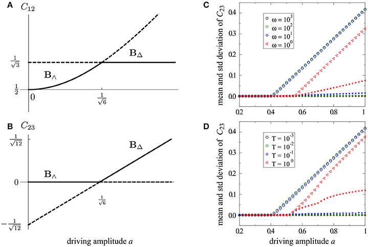
Figure 2. Bifurcation diagrams for the 3-node model (Figure 1B). Analytical solutions for periodic driving are shown in (A,B), including stable (solid) and unstable (dashed) branches. Simulated behavior for the shunting conductance C₂₃ is shown for periodic driving (C) and rapid stochastic driving (D). Mean values (large open symbols) and standard deviation (small filled symbols) are measured for C₂₃(t) over the entire simulation. For both periodic and stochastic driving the predicted bifurcation point $a_{\text{c}}\to 1/\sqrt{6}$ is asymptotically reached as the characteristic driving frequency T⁻¹ → ∞.

3.3. One Source and Multiple Fluctuating Sinks (Augmented Tree, H > 1)

Let us now turn to larger systems with more than two sinks and nodes representing intermediate branching points between source and sinks. The networks considered are complete binary trees, augmented with cross edges directly at each branching, shown as dashed edges in Figure 1C. We consider the stationary conductance values under stochastic driving with a rapid characteristic time scale T ≪ 1.

For a level l ∈ {0, 1, …, H} in a system with height H, we consider the dynamics for conductances of tree-edges, $C_{\wedge }^{(l,H)}$, and of cross-edges, $C_{-}^{(l,H)}$, see Figure 1C. By $a_{\text{c}}^{(l,H)}$ we denote the critical driving amplitude above which cross-edges with non-zero conductances emerge. Figure 3 shows the asymptotic values of the conductances of cross-edges for fluctuations with varying amplitude a. Non-zero conductances in cross-edges appear with increasing amplitude in an order that follows the hierarchy of the tree, i.e., $a_{\text{c}}^{(k,H)}>a_{\text{c}}^{(l,H)}$ for all 0 ≤ k < l < H. To illustrate, as we increase a, the cross-edges between sinks, l = H, are the first that begin to conduct. Then as we increase a even further, the next level, l = H − 1, obtains conducting cross-edges, and so on. Accordingly, the last transition to non-zero conductance for increasing amplitude a occurs in $C_{-}^{(1,H)}$ between the root's child nodes.

FIGURE 3

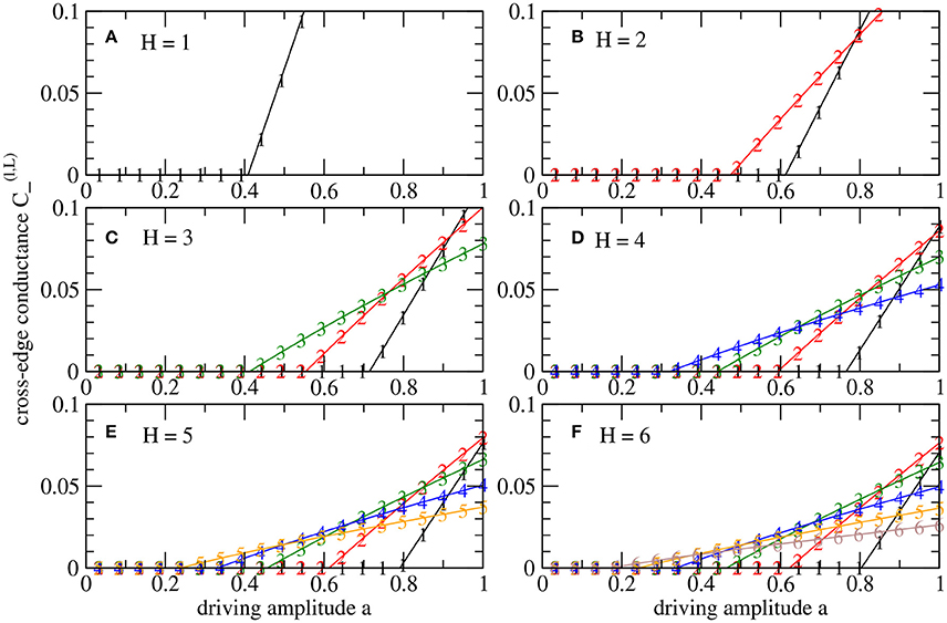
Figure 3. Bifurcation diagrams for augmented tree systems (H > 1) according to Figure 1C with dynamics under fast stochastic driving at the sinks. The conductances of cross-edges are shown for different levels l as defined in Figure 1, i.e., from the root (l = 0) to the sinks in the leaves (l = H). The values result from parameter scans decreasing driving amplitude a from 1 to 0. (A–F) Distinguish systems with different heights H ∈ {1, 2, …, 6}. In each case, the number of nodes is N = 2^{H + 1} − 1, i.e., N = 127 nodes for H = 6.

One may speculate if all observed transitions from zero to non-zero conductance are of the same kind at different levels, only varying in the parameter value $a_{\text{c}}^{(l,H)}$ at the transition and the slope in the supercritical regime. Figure 4 shows that this is indeed the case for the cross-edge at level l = 1. Plotting the conductances of the edges of the source node as a function $a/a_{\text{c}}^{(l,H)}$, we observe a perfect collapse of all data for varying H (and l = 1 fixed), by rescaling $a\mapsto a/a_{\text{c}}^{(l,H)}=:ã$ in systems of different heights H. So the top triangle including the source node of an augmented tree of general height H behaves in the same way as the H = 1 system with driving parameter a rescaled. Thus, the analytic results Equations (28) and (29) for H = 1 allow us to express the scaled conductances explicitly,

$\begin{array}{cc}{\tilde{C}}_{12}{|}_{l=1}=\frac{1}{2}\sqrt{1+\frac{1}{3}{\tilde{a}}^2},& (33)\end{array}$

$\begin{array}{cc}{\tilde{C}}_{23}{|}_{l=1}=\frac{1}{\sqrt{12}}(\tilde{a}-1).& (34)\end{array}$

FIGURE 4

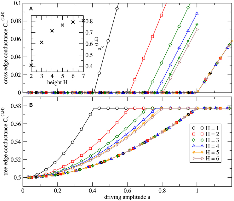
Figure 4. Parameter dependence of stationary conductances in the top triangle of systems with height H. Open symbols denote in (A) the conductance of the root's tree edges, $C_{\wedge }^{(1,H)}$, and in (B) the conductances of the root's cross-edge, $C_{-}^{(1,H)}$. Filled symbols are the same values plotted as a function of a rescaled with the critical value $a_{\text{c}}^{(1,H)}$. The inset in (A) shows the critical values $a_{\text{c}}^{(1,H)}$. For height H, the system has N = 2^H+1 − 1 nodes, i.e., N = 127 nodes for H = 6.

The a-dependence of conductances on the other levels is more intricate, as is shown in Figure 5 for the case of a system with H = 6 levels. The derivatives of cross-edge conductances reveal detail not apparent in the coarser plot (Figure 3) of these conductances themselves. The slope is maximal at the transition (as the one-sided derivative with a approaching a_c(l, 6) from above). As a is increasing, the conductance curve becomes slightly flatter. This non-linear effect hints at dependencies between the levels, l. However, one may show that using the same rescaled amplitude parameter, ã, and then $C_{\wedge }^{(l,H)}$ and $C_{-}^{(l,H)}$ collapse to single curves for fixed l while varying H (not shown).

FIGURE 5

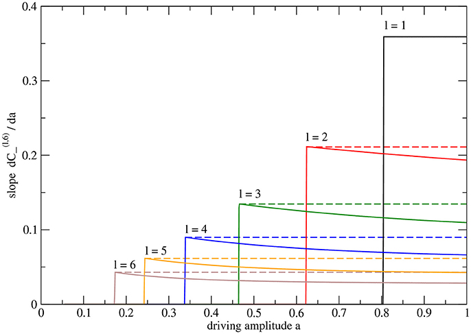
Figure 5. Slopes of conductances of cross edges in the system with height H = 6 with n = 64 sinks and N = 127 nodes in total. The plotted curves are the numerically determined derivatives of the data plotted in Figure 3F. For each curve, the maximum value is indicated by an extra vertical dashed line. Note that the derivative is piecewise constant only for the cross edge closest to the root. The other conductances exhibit maximal slope only at the critical point.

The Supplementary Material of this article provides four videos of simulations of the dynamics for systems with height H = 4. Each of these shows a parameter sweep as described in section 2.6. Supplementary Video 1 (297323_Martens_Video 1.MP4) shows the dynamics for the network structure studied above, i.e., with one cross edge at each branching as illustrated in Figure 1C. Supplementary Video 2 (297323_Martens_Video 2.MP4), the tree is further augmented to allow for cross edges bridging longer distances in the tree; such a network structure is shown in Figure 1D. Two further Supplementary Videos 3, 4 (297323_Martens_Video 3.MP4, 297323_Martens_Video 4.MP4) employ damaged versions of the latter structure in which roughly half of all cross edges have been randomly selected and removed. These simulations confirm the observation that the cross edges begin to conduct in order of the tree hierarchy, starting from sinks and moving toward the source.

4. Discussion and Outlook

We have studied how fluctuating loads affect the re-configuration of vessels in an adaptive flow network. To do this, we have introduced a minimal model, consisting of a resistive network with conductances on the edges which adapt dynamically toward minimizing fluctuations in the network. To be explicit, the conductance is up-regulated with the pressure drop squared (power dissipated), but down-regulated with a factor proportional to the conductance. Although adaptation adheres to local rules they also experience a global feedback through the coupling via the flow network. An important question, which also appears in the context of synaptic plasticity [35], is then: what are the (stable) equilibrium configurations of conductance in the network? Furthermore, we introduced load fluctuations by including fluctuating sinks in certain network nodes. For a characteristic time scale T of the fluctuations much more rapid than the time scale of adapting conductances, T ≪ 1, we can treat fluctuations in terms of their averages over time, i.e., their amplitudes. Considering both periodic and stochastic fluctuations, we analytically and numerically investigated small and large networks to determine how their equilibrium conductance configurations depends on the amplitude of the load fluctuations, a. In particular, we used this model to investigate how far into the network the fluctuations would be able to induce re-configurations.

First, we investigated two very simple network motifs regarding the space of equilibrium configurations and their stability. The dynamics for the motif consisting of one fluctuating sink and source can be solved exactly (Figure 1A). The conductance connecting the two nodes is non-zero and stable for all fluctuation amplitudes with a > 0. The triangular motif with one constant source and two fluctuating sinks (Figure 1B) can also be solved analytically, but exhibits a transcritical bifurcation at a critical drive amplitude a_c: for sub-critical drive, a < a_c, the tree-like solution branch without cross edge is stable; for super-critical drive, a > a_c, the cyclic structure (triangle with non-zero tree-edge and cross-edge) is stable, see Figure 2. Numerical simulations demonstrate that the system behavior asymptotically approaches the solutions obtained for the limit of rapid driving (T → 0) as T → ∞.

Next, we ran numerical simulations of larger tree-like networks with a constant source at its root and fluctuating loads in the leaves. Using an initial configuration C_ij|_{t = 0} = 1 for all edges (i, j) ∈ A, we then investigated into which quasi-stationary configuration the network settles. To investigate the system behavior analytically, we studied two scenarios. First, we assumed a simplified network structure, i.e., a complete binary tree with cross-edges only at each branching, see Figure 1C and Supplementary Video 1. Conductances $C_{-}^{(l,H)}$ of cross-edges undergo a transition at a critical driving amplitude. We find $C_{-}^{(l,H)}>0$ for a > a_c(l, H), and $C_{-}^{(l,H)}=0$ for a ≤ a_c(l, H). The critical driving amplitudes a_c(l, H), depending on the edge level l and height H of the tree-like structure, are hierarchically ordered so that the transitions to non-zero cross-edge conductances appear successively in descending order of l as the amplitude grows. Thus, we observe that as the amplitude is increased cycles first emerge near the fluctuating sinks and then spread toward the root with the constant source. Second, we compared these observations with the behavior in a generalized network topology. In this second scenario, we ran numerical simulations of networks lacking intrinsic tree structure, i.e., where all cross-edges are allowed, see Figure 1D and Supplementary Video 2. In this case, the threshold for an edge (i, j) between sinks i and j has a dependency on the length of the tree path between i and j. The longer the tree path (distance on tree), the lower its threshold. This means that—as the amplitude is increased—minimal distance short-cuts for longer paths form before the cross-edges from the first scenario. In both scenarios, however, the network is partitioned into two regions with tree-like motifs near the source at the root and cycles closer to the fluctuating sinks in the leaves of the tree. Transitions get more complicated when randomly chosen cross-edges are topologically deleted (Supplementary Videos 3, 4).

Other work has investigated the appearance of cyclic structures (loops) by discussing flow networks via optimization in terms of minimizing dissipative losses under continuous reconfiguration of the flow conditions [19, 20, 28]. While this point of view may be motivated by evolutionary principles and yielded many interesting insights regarding the critical emergence of cycles, we were interested in formulating a minimal dynamical model [36]. Contrasting previous studies, we did not assume spatially uniform fluctuations and investigate conditions under which cyclic structures form in general; rather, we investigated if partitions between tree-like and cyclic structures would form and where their boundaries lie. Many studies in vascular physiology focused on the dynamics of single vessels and have complex biophysical models including a large degree of complexity prohibitive to mathematical analysis, and only few have computationally investigated dynamics in networks [30, 32]; here, we tried to systematically address stability of such vessel models from a mathematical perspective.

The study on simple network motifs has been insightful and complemented the numerical findings that we have made for larger trees. Further research may address equilibrium configurations and their transitions ($a_c^{(l,H)}$) from tree-like to cyclic structures in network structures shown in Figures 1C,D, and attempt to find complete solutions via mathematical analysis and scaling arguments. For the case of more general network topologies (see e.g., Figure 1D and for the case of heterogeneities, an open question remains whether multi-stable equilibria are possible. Furthermore, research should be conducted on reducing complex biophysical dynamics to simpler mathematical models, which could be investigated toward identifying classes of different dynamic behavior. Finally, generalizations to co-evolving networks with edges being dynamically created/deleted may be considered [37].

Author Contributions

All authors listed, have made substantial, direct and intellectual contribution to the work, and approved it for publication.

Funding

We acknowledge travel funding from Action CA15109, European Cooperation for Statistics of Network Data Science (COSTNET). Research conducted by EM is supported by the Dynamical Systems Interdisciplinary Network, University of Copenhagen. KK acknowledges funding from MINECO through the Ramón y Cajal program and through project SPASIMM, FIS2016-80067-P (AEI/FEDER, EU).

Conflict of Interest Statement

The authors declare that the research was conducted in the absence of any commercial or financial relationships that could be construed as a potential conflict of interest.

Acknowledgments

EM would like to thank J. C. Brings Jacobsen for helpful discussions on circulatory physiology and E. Katifori on adaptive networks.

Supplementary Material

The Supplementary Material for this article can be found online at: https://www.frontiersin.org/articles/10.3389/fphy.2017.00062/full#supplementary-material

Supplementary Material for this article consists of 4 Videos (1–4) which are described at the end of section 3.3. A legend for the conductances is supplied in Image 1.

Footnotes

1. ^In parts of the literature, the term loop is used synonymous with cycle. Loop, however, may also refer to an edge connecting a node with itself [34].

2. ^Note that periodic driving may be generalized to larger spanning trees with N = 2^L > 3 where L denotes the number of branching levels: $h_l=-\frac{1}{2}\pm a^{l\text{ mod }2}\text{ cos }\omega t$ where l = 2^L−1 + 1, …2^L are indices for the leafs of the tree. Thus, there are (2^L − 2^L−1)/2 pairs of leaves that balance each other. To break the symmetry, we may permute the leaf indices l in h_l.

3. ^To be precise, for moderately small T, the conductance C₁₂ oscillates around 〈C₁₂〉, with an amplitude that vanishes as T → 0.

References

1. Strogatz SH. Exploring complex networks. Nature (2001) 410:268–76. doi: 10.1038/35065725

PubMed Abstract | CrossRef Full Text | Google Scholar

2. Hufnagel L, Brockmann D, Geisel T. Forecast and control of epidemics in a globalized world. Proc Nat Acad Sci USA (2004) 101:15124–9. doi: 10.1073/pnas.0308344101

PubMed Abstract | CrossRef Full Text | Google Scholar

3. Brockmann D, Hufnagel L, Geisel T. The scaling laws of human travel. Nature (2006) 439:462–5. doi: 10.1038/nature04292

PubMed Abstract | CrossRef Full Text | Google Scholar

4. Barabási AL, Oltvai ZN. Network biology: understanding the cell's functional organization. Nat Rev Genet. (2004) 5:101–13. doi: 10.1038/nrg1272

PubMed Abstract | CrossRef Full Text | Google Scholar

5. Kaluza P, Kölzsch A, Gastner MT, Blasius B. The complex network of global cargo ship movements. J R Soc Interf. (2010) 7:1093–103. doi: 10.1098/rsif.2009.0495

PubMed Abstract | CrossRef Full Text | Google Scholar

6. Travers J, Milgram S. The small world problem. Psychol Today (1967) 1:61–7.

Google Scholar

7. Marbach S, Alim K, Andrew N, Pringle A, Brenner MP. Pruning to increase taylor dispersion in physarum polycephalum networks. Phys Rev Lett. (2016) 117:1–5. doi: 10.1103/PhysRevLett.117.178103

PubMed Abstract | CrossRef Full Text | Google Scholar

8. Devor A, Tian P, Nishimura N, Teng IC, Hillman EMC, Narayanan SN, et al. Suppressed neuronal activity and concurrent arteriolar vasoconstriction may explain negative blood oxygenation level-dependent signal. J Neurosci. (2007) 27:4452–9. doi: 10.1523/JNEUROSCI.0134-07.2007

PubMed Abstract | CrossRef Full Text | Google Scholar

9. Jacobsen JCB, Hornbech MS, Holstein-Rathlou NH. A tissue in the tissue: models of microvascular plasticity. Eur J Pharm Sci. (2009) 36:51–61. doi: 10.1016/j.ejps.2008.09.012

PubMed Abstract | CrossRef Full Text | Google Scholar

10. Feldberg R, Colding-Jørgensen M, Holstein-Rathlou NH. Analysis of interaction between TGF and the myogenic response in renal blood flow autoregulation. Am J Physiol. (1995) 269(4 Pt 2):F581–93.

PubMed Abstract | Google Scholar

11. Alstrøm P, Eguíluz VM, Colding-Jørgensen, F M, Gustafsson, and Holstein-Rathlou NH. Instability and “Sausage-String” appearance in blood vessels during high blood pressure. Phys Rev Lett. (1999) 82:1995–8. doi: 10.1103/PhysRevLett.82.1995

CrossRef Full Text | Google Scholar

12. Jacobsen JCB, Gustafsson F, Holstein-Rathlou NH. A model of physical factors in the structural adaptation of microvascular networks in normotension and hypertension. Physiol Meas. (2003) 24:891–912. doi: 10.1088/0967-3334/24/4/007

PubMed Abstract | CrossRef Full Text | Google Scholar

13. VanBavel E, Tuna BG. Integrative modeling of small artery structure and function uncovers critical parameters for diameter regulation. PLoS ONE (2014) 9:e86901. doi: 10.1371/journal.pone.0086901

PubMed Abstract | CrossRef Full Text | Google Scholar

14. Kassab GS, Rider CA, Tang NJ, Fung YC. Morphometry of pig coronary arterial trees. Am J Physiol. (1993) 265(1 Pt 2):H350–65.

PubMed Abstract | Google Scholar

15. Reichold J, Stampanoni M, Keller AL, Buck A, Jenny P, Weber B. Vascular graph model to simulate the cerebral blood flow in realistic vascular networks. J Cereb Blood Flow Metab. (2009) 29:1429–43. doi: 10.1038/jcbfm.2009.58

PubMed Abstract | CrossRef Full Text | Google Scholar

16. Kassab GS. Scaling laws of vascular trees: of form and function. Am J Physiol Heart Circul Physiol. (2006) 290:894–903. doi: 10.1152/ajpheart.00579.2005

PubMed Abstract | CrossRef Full Text | Google Scholar

17. Blinder P, Tsai PS, Kaufhold JP, Knutsen PM, Suhl H, Kleinfeld D. The cortical angiome: an interconnected vascular network with noncolumnar patterns of blood flow. Nat Neurosci. (2013) 16:889–97. doi: 10.1038/nn.3426

PubMed Abstract | CrossRef Full Text | Google Scholar

18. Ronellenfitsch H, Timme M, Witthaut D. A dual method for computing power transfer distribution factors. IEEE Trans Power Syst. (2017) 32:1007–15. doi: 10.1109/TPWRS.2016.2589464

CrossRef Full Text | Google Scholar

19. Dodds PS. Optimal form of branching supply and collection networks. Phys Rev Lett. (2010) 104:048702. doi: 10.1103/PhysRevLett.104.048702

PubMed Abstract | CrossRef Full Text | Google Scholar

20. Corson F. Fluctuations and redundancy in optimal transport networks. Phys Rev Lett. (2010) 104:048703. doi: 10.1103/PhysRevLett.104.048703

PubMed Abstract | CrossRef Full Text | Google Scholar

21. Rubido N, Grebogi C, Baptista MS. Resiliently evolving supply-demand networks. Phys Rev E (2014) 89:1–5. doi: 10.1103/PhysRevE.89.012801

PubMed Abstract | CrossRef Full Text | Google Scholar

22. Farr RS, Harer JL, Fink TMa. Easily repairable networks: reconnecting nodes after damage. Phys Rev Lett. (2014) 113:138701. doi: 10.1103/PhysRevLett.113.138701

PubMed Abstract | CrossRef Full Text | Google Scholar

23. Tero A, Takagi S, Saigusa T, Kentaro I, Bebber DP, Fricker MD, et al. Rules for biologically inspired adaptive network design. Science (2010) 327:439–43. doi: 10.1126/science.1177894

PubMed Abstract | CrossRef Full Text | Google Scholar

24. Kantorovich LV. On the translocation of masses. Doklady Akademii Nauk SSSR (1942) 37:199–201.

25. Villani C. Topics in Optimal Transportation, vol. 58. Providence, RI: American Mathematical Society (2003).

Google Scholar

26. Bohn S, Magnasco MO. Structure, scaling, and phase transition in the optimal transport network. Phys Rev Lett. (2007) 98:3–6. doi: 10.1103/PhysRevLett.98.088702

PubMed Abstract | CrossRef Full Text | Google Scholar

27. Durand M. Structure of optimal transport networks subject to a global constraint. Phys Rev Lett. (2007) 98:1–4. doi: 10.1103/PhysRevLett.98.088701

PubMed Abstract | CrossRef Full Text | Google Scholar

28. Katifori E, Szőllősi GJ, Magnasco MO. Damage and fluctuations induce loops in optimal transport networks. Phys Rev Lett. (2010) 104:048704. doi: 10.1103/PhysRevLett.104.048704

PubMed Abstract | CrossRef Full Text | Google Scholar

29. Gross T, Blasius B. Adaptive coevolutionary networks: a review. J R Soc Interf. (2008) 5:259–71. doi: 10.1098/rsif.2007.1229

PubMed Abstract | CrossRef Full Text | Google Scholar

30. Hacking WJ, VanBavel E, Spaan JA. Shear stress is not sufficient to control growth of vascular networks: a model study. Am J Physiol. (1996) 270(1 Pt 2):H364–75.

PubMed Abstract | Google Scholar

31. Lee DS, Rieger H, Bartha K. Flow correlated percolation during vascular remodeling in growing tumors. Phys Rev Lett. (2006) 96:058104. doi: 10.1103/PhysRevLett.96.058104

PubMed Abstract | CrossRef Full Text | Google Scholar

32. Postnov DD, Marsh DJ, Postnov DE, Braunstein TH, Holstein-Rathlou NH, Martens EA, et al. Modeling of kidney hemodynamics: probability-based topology of an arterial network. PLoS Comput Biol. (2016) 12:e1004922. doi: 10.1371/journal.pcbi.1004922

PubMed Abstract | CrossRef Full Text | Google Scholar

33. Farquhar GD, Cowan IR. Oscillations in stomatal conductance. Plant Physiol. (1974) 54:769–72. doi: 10.1104/pp.54.5.769

PubMed Abstract | CrossRef Full Text | Google Scholar

34. Diestel R. Graph Theory, vol. 173 of Graduate Texts in Mathematics, 4th Edn. Berlin, Heidelberg: Springer (2012).

35. Tetzlaff C, Kolodziejski C, Timme M, Wörgötter F. Synaptic scaling in combination with many generic plasticity mechanisms stabilizes circuit connectivity. Front Comput Neurosci. 5:47. doi: 10.3389/fncom.2011.00047

PubMed Abstract | CrossRef Full Text

36. Gräwer J, Modes CD, Magnasco MO, Katifori E. Structural self-assembly and avalanchelike dynamics in locally adaptive networks. Phys Rev E (2015) 92:012801. doi: 10.1103/PhysRevE.92.012801

PubMed Abstract | CrossRef Full Text | Google Scholar

37. Taylor-King JP, Basanta D, Chapman SJ, Porter MA. A mean-field approach to evolving spatial networks, with an application to osteocyte network formation. arXiv 2017;1702.00759.