Behavioral Heterogeneity Affects Individual Performances in Experimental and Computational Lowest Unique Integer Games

1. Introduction

In social and economic systems, individuals, groups, firms and so on make their decision based on the rules they should obey. For example, call market, continuous double auction and other trading mechanisms are seen in financial markets and investors trade by taking into consideration which mechanism is introduced [2]. Or, first- and second-prize styles are usually employed in auction markets and the theoretical bid is different from the auction style [3]. On the other hand, new types of social and economic systems have been also proposed and some of them are introduced in practice. Among these, Swedish lottery (SL) game Limbo and Lowest/Highest Unique Bid Auctions (LUBA/HUBA) like the Auction Air or Juubeo websites are one of the new systems where the participants are required to be unique by taking risks of not being so.

Lowest Unique Integer Games (LUIGs) are highly simplified versions of SL and LUBA/HUBA. In a LUIG, N (≥ 3) players simultaneously submit a positive integer up to M. The player choosing the smallest number that is not chosen by anyone else is the winner. In cases where no player chooses a unique number, there is no winner. For instance, suppose there is a LUIG with N = 3 and M = 3. There are three players, A, B, and C, who each submit an integer between 1 and 3. If the integers chosen by A, B, and C are 1, 2, and 3, respectively, then A wins the game. If the integers chosen by A, B, and C are 1, 1, and 2, respectively, then C is the winner. And, as noted, if all of them choose the same integer, there is no winner.

LUIGs are more tractable than the above-mentioned real systems because the exact numbers of players or participants and the options are known for their decision-making. In this sense, these types of real systems have been attracting much attention recently from scholars of various disciplines¹. In addition, several social or economic systems have characteristics of LUIGs. As Östling et al. [4] have pointed out, “choices of traffic routes and research topics, or buyers and sellers choosing among multiple markets” (p. 3) are probable examples. Or, the Braess paradox can be explained by LUIG [1]. While the previous studies have investigated these related systems theoretically and empirically, the behaviors of the bidders and participants, and the dynamics of game outcomes are not so clear. Likewise, experimental studies on LUIGs and related systems are still scarce except for Östling et al. [4] and Rapoport et al. [5]. Östling et al. have conducted a laboratory experiment of SL and found that there are mainly four kinds of behaviors observed: random, stick, lucky and strategic. Based on their findings, Mohlin et al. have proposed two learning models, global cumulative imitation and similarity-based imitation, where players make use of not only their choice but also the game outcome for updating their attractions [6]. On the other hand, Rapoport et al. have experimentally studied a version of LUBA/HUBA with (N, M) ∈ {(5, 4), (5, 25), (10, 25)} and found that only a small fraction of subjects behaved as theoretically predicted [5].

Yamada and Hanaki experimentally studied LUIGs to determine if and how subjects self-organized into different behavioral classes to obtain insights into choice patterns that can shed light on the alleviation of congestion problems [1]. They considered four LUIGs with N = {3, 4} and M = {3, 4} and implemented a laboratory experiment for totally 192 subjects. Each subject played two separate LUIGs but the difference between the two LUIGs was either N or M. Therefore, each LUIG had 96 subjects and they were equally split into two parties, those who played it in Game 1 and the others who did in Game 2². Accordingly, 48 subjects played one of the four LUIGs in Game 1, which yielded 16 groups in three-person LUIGs and 12 groups in four-person LUIGs. Yamada and Hanaki found that (a) choices made by more than 1/3 of subjects were not significantly different from what a symmetric mixed-strategy Nash equilibrium (MSE) predicts; however, (b) subjects who behaved significantly differently from what the MSE predicts won the game more frequently.

These early experimental studies suggest that the strategy and the decision-making of subjects are heterogeneous and that the theoretical predictions may not be effective to win more. Yet, due to limited number of samples, it is necessary to intensively examine the relations between the behavior and learning of individuals, which can be an origin of heterogeneity, and their performances. This study extends their past experimental work to check whether such successful or unsuccessful behaviors are also true for the game with different opponents. For this purpose, the author pursues computational approach where the calibrated agents play with all agents including themselves (round robin contest) and make comparison between experimental and computational experiments. Here, several typical learning models are employed to express the behaviors of subjects in the laboratory experiment. Then, the one with the best likelihood for every subject in each game setup is used for computational experiments.

Several studies have employed both experimental and computational approaches to computationally test the experimental results and vice versa. According to Duffy, its advantages are summarized as “the agent-based approach to understand results obtained from laboratory studies with human subjects” and “to understand findings from agent-based simulations with follow-up experiments involving human subjects” (p. 951) [7]. The necessity of combining two approaches have been argued and the methodology has been proposed for the last decade (e.g., [8–11]). There are a few researches which indeed employ the combined approach to computationally test the validity of experimental findings in the laboratory, implement an intensive computational experiment, and extend the experimental design by using the laboratory data [12–14].

2. Materials and Methods

In the laboratory experiment by Yamada and Hanaki [1], they observed that keeping on choosing a number was an effective way to win LUIGs. But, it was not at that moment sure whether such sticking behavior was really successful. Here, a computational experiment of round robin competition is employed to see its effectiveness. Before the competition, several typical learning models are employed and the parameters of the models for each subject are then estimated.

2.1. Learning Models

The learning models are as follows:

• One variable adaptive learning (AL1)

An AL1 player i has a propensity $a_i^k(t)$ for number k (k = 1, ⋯, M) at the beginning of round t. Before the start of a game, she is assumed to have the same non-negative propensities for all the possible integers, namely $a_i^j(0)=a_i^k(0)\ge 0\mathrm{\text{for}}j\ne k$.

In every round, she chooses one integer according to the following exponential selection rule

$p_i^k(t)=\frac{exp({\lambda }_a·a_i^k(t))}{{\displaystyle {\sum }_{k^{\prime }=1}^M}exp({\lambda }_a·a_i^{k^{\prime }}(t))}$

where $p_i^k(t)$ is i's selection probability for integer k in round t, and λ_a is a positive constant called sensitivity parameter ([15, 16]).

After a round, propensities are updated as

$a_i^k(t+1)=(1-{\varphi }_a)a_i^k(t)+1_{\left\{k,s_i(t)\right\}}{\psi }_{a}R$

where ϕ_a and ψ_a are positive constants called learning parameter ([15, 16]), 1_{·} is the indicator function that takes 1 if k = s_i(t), and 0 otherwise. Here s_i(t) is the number that player i has actually chosen in round t, and R is the payoff received. Note that the model is called “cumulative” if ψ_a = 1 and “averaging” if ψ_a = ϕ_a.

• Three variables adaptive learning (AL3)

Players using this model take into consideration two additional psychological assumptions, experimentation and forgetting. Here, propensities are updated as

$a_i^k(t+1)=(1-{\varphi }_b)a_i^k(t)+1_{\left\{k,s_i(t)\right\}}{\psi }_{b}R$

when they win and

$a_i^j(t+1)=(1-{\varphi }_b)a_i^j(t)+{\psi }_bϵR/(M-1)(j\ne s_i(t))$

when they lose³. ϕ_b and ψ_b are also learning parameters and ϵ is a experimentation parameter. Here ϵ is set to 1.0.

• Naive imitation (NI)

Players using this model follow a winning number regardless of whether they are a winner or not. When “no-winner” situation happens, they choose the preceding number⁴.

While the selection rule is the same as that in AL1 and AL3 models, the updating rule is expressed in the following:

$a_i^k(t+1)=(1-{\varphi }_n)a_i^k(t)+1_{\left\{k,v(t)\right\}}{\psi }_{n}R$

where v(t) is a winning number in round t, and ϕ_n and ψ_n are also learning parameters.

• Stick

Players using this model always choose only one number⁵.

2.2. The Data to Calibrate

Since the subjects in the earlier laboratory experiment were asked to choose and submit one of the M integers, the experimental data for calibration include rounds, the choices of subjects and the winning number for every group in every LUIG. In other words, they were not asked to imagine what numbers their opponents would choose or to determine the probability distribution so that one number would be randomly chosen.

To determine a learning model for every subject, the author set one condition and assumed one point: First, only the experimental data in Game 1 were used for calibration. This is because learning across the games cannot be clearly treated. For example, when subjects play a LUIG with M = 3 in Game 1 and that with M = 4 in Game 2, it is not clear how the initial propensity for the integer 4 is given. Besides, even if the calibration is done, it is not preferable that the initial state is different from the subjects; Second, all initial propensities in Game 1 are set to zero, namely the subjects did not have any prior belief to others or view to the game. Then, the learning model with the best log likelihood is employed for the simulation⁶. Note that the subjects who did not change at all in Game 1 belong to “stick.”

2.3. Computational Round Robin Contest

The experimental design is as follows:

1. Agents played the same LUIG as the corresponding subjects played in the laboratory.

2. Every agent competes all the combinations of opponents including him/herself. Therefore, the total number of combinations is ₄₈H_N and an agent faces 1,174 (three-person LUIGs) and 29,329 (four-person LUIGs) patterns of opponents.

3. Every combination of agents played the LUIG 100 times each of which has 50 rounds.

4. The initial propensities of each agent in each game are the ones estimated by the maximum likelihood method. In other words, the agents learn and update their belief by using the data of Yamada and Hanaki [1] before they start to play the computational LUIG.

5. The information available for the agents is their choice and the winning number in the preceding round. However, at the beginning of each game, there does not exist the winning number.

6. Agents learn according to their calibrated learning model with the corresponding parameters.

All numerical results in the next section have been computed in double precision on a 2.4 GHz PC with 8 GB of RAM and a linux OS (Kernel 4.4.52-2vl6). All the source codes have been written in C++, and complied and optimized by GNU g++ version 4.9.3⁷.

3. Results

3.1. Classification of Subjects

Before discussing the results of computational round robin competitions, the author needs to pay attention to how the subjects were classified and whether there are relations between their calibrated learning model and their behaviors observed in the laboratory.

Table 1 shows the relation between the calibrated learning model and the choice and the change criteria given in Yamada and Hanaki [1]⁸. Two updating rules, cumulative and averaging, are encapsulated into one. Cramer's coefficient of association for each LUIG is also given. Note that the abbreviation “LUIG34” means that the number of players N is 3 and the upper limit M is 4. Thus, the first number followed by “LUIG” is N and then M comes next.

TABLE 1

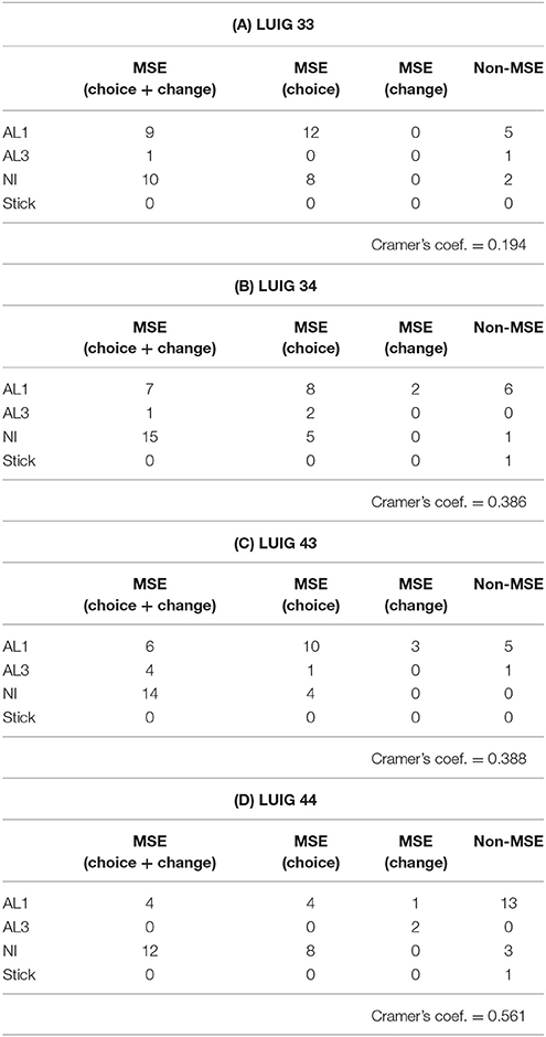
Table 1. Classification of subjects by observed behavior in the laboratory and the estimated learning model.

Cramer's coefficient of association seems to depend on both N and M. When N and M are small, the value is relatively low (0.193 for LUIG 33). On the other hand, if N and/or M are large, the coefficient becomes larger. In particular, Cramer's coefficient of association for LUIG 44 is 0.561, namely many of the subjects who played not differently from MSE prediction are considered as NI players whereas those who deviated from the MSE prediction took into account only their own choices. This means, since larger N and M make it more difficult to imagine what number one's opponents chose from his/her choice and the winning number, some of the subjects became to rely on the available information.

Next, the author takes a look at how the subjects in the laboratory would have played if the game had continued. To answer this question, the author employed cluster analysis. By doing so, the expected behaviors of subjects would be quantitatively categorized and characterized.

To conduct the analysis, the following procedure was employed: First, the propensities in round 50 of laboratory experiment were calculated by using the game log. Second, the probability to choose each integer in round 51 was obtained. Third, the updated choice probability was calculated for all the possible cases. Here, “case” means that a subject's choice is k and the winning number is w. Accordingly, there are totally M(M+1) cases in a LUIG. Lastly, the author set the following values as inputs:

• Submission probability for integer k (k = 1, ⋯, M) in round 51

• The following inputs are calculated for all k:

• Updated probability to choose the same integer in round 52 when there are no winner in round 51

• Updated probability to choose the same integer in round 52 when s/he wins in round 51

• Updated probability to choose the same integer in round 52 when s/he loses in round 51

• Updated probability to choose the winning integer in round 52 when s/he loses in round 51

After having a dendrogram⁹ in each LUIG, the author split them into four or five clusters and obtained the inputs of “median” agents in each cluster¹⁰ (Figures 1–4).

FIGURE 1

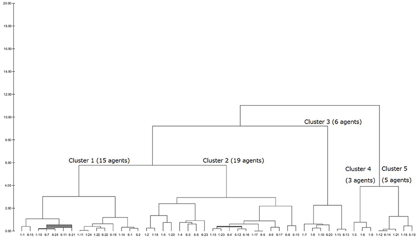
Figure 1. Generated dendrogram (LUIG33).

FIGURE 2

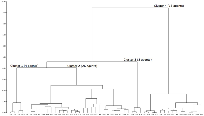
Figure 2. Generated dendrogram (LUIG34).

FIGURE 3

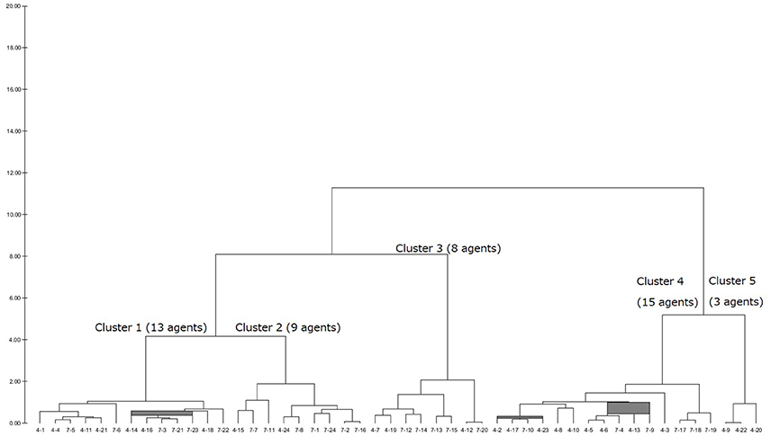
Figure 3. Generated dendrogram (LUIG43).

FIGURE 4

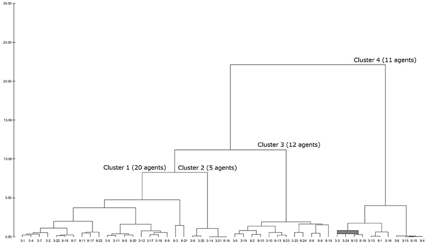
Figure 4. Generated dendrogram (LUIG44).

Table 2 summarizes how the representative agents in each cluster would play and update their propensities in round 51¹¹.

TABLE 2

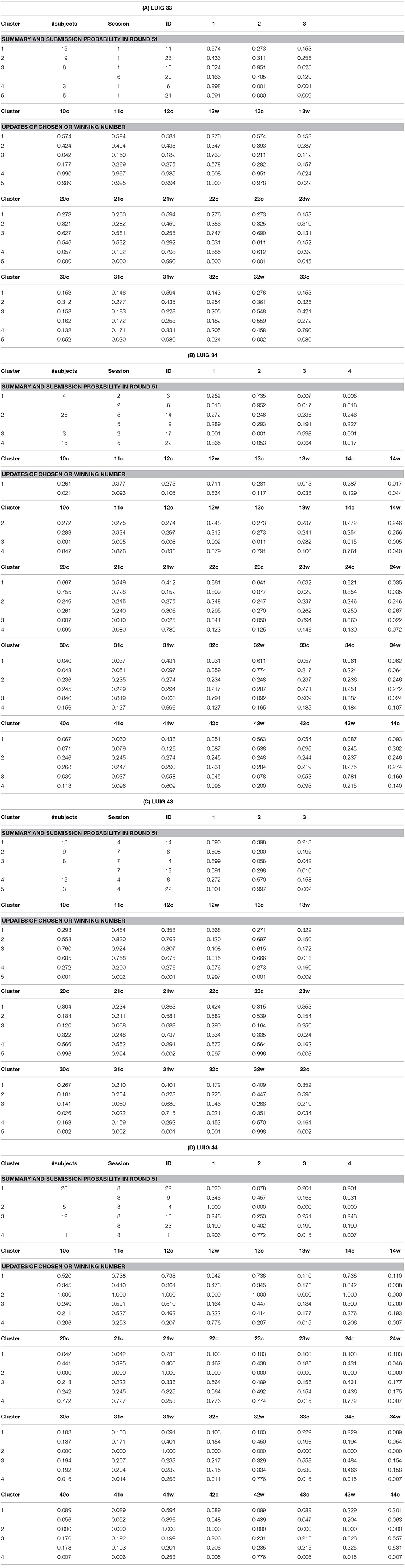
Table 2. Expected behaviors of representative agents in each cluster (ID: Subject ID in the session).

There are mainly three choice patterns observed: keeping on choosing one number, completely or relatively randomized behavior with fluctuation, and completely or relatively randomized behavior with non-fluctuation. The first pattern includes sticking behavior and a result of reinforcement. The remaining two patterns stem from the fact that the corresponding subjects failed to reinforce their propensities and that they were sensitive to the winning number. In addition, the value of sensitivity parameter was small so that every number was equally chosen anytime. Hence, whether sticking to a number or not played an important role in LUIGs, which may support the results of the earlier laboratory experiment.

3.2. Experimental Results

Agents in the round robin competition faced all the agents including his/herself. By doing so, the author compares their performances between when they played with different opponents and when their opponents included themselves.

Table 3 shows the summary statistics of each LUIG in terms of the agent structure. The data include the frequency of game outcomes, the number of wins, that of changes, and Pearson' correlation between the numbers of wins and changes. This table also provides with the results of laboratory experiment and the theoretical prediction for comparison. The partitions of agents are in the following:

• Three-person LUIGs

• 3

Three identical agents exist;

• 2–1

Two identical agents and one different agent exist; and

• 1–1–1

Three different agents exist.

• Four-person LUIGs

• 4

Four identical agents exist;

• 3–1

Three identical agents and one different agent exist;

• 2–2

Two different pairs of two identical agents exist;

• 2–1–1

Two identical agents and two other different agents exist and;

• 1–1–1–1

Four different agents exist.

TABLE 3

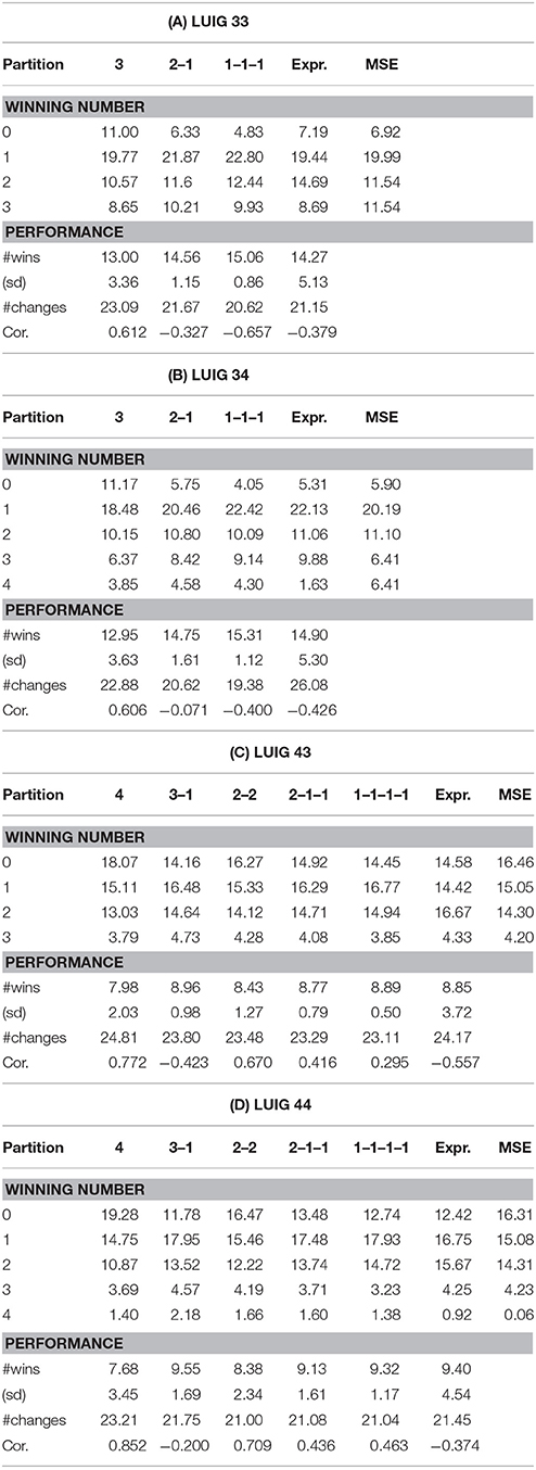
Table 3. Summary statistics of round robin competition in computational experiments.

The cases where there are identical agents mean that they played with one or more agents whose learning model and its values of parameters were the same. But the updating process is different. And the different agents mean at least their learning model or its values of parameters is/are different from those of the others in the group.

The above partitions of agents are related to behavioral heterogeneity. When heterogeneity is high, “no-winner” situations were less frequently observed and thereby the average number of wins became larger. This is especially true for three-person LUIGs. In four-person LUIGs, things are a little bit different; When there are only two kinds of agents and one agent is singular, the average number of wins per agent is about 8.96 (LUIG43) and 9.55 (LUIG44). Meanwhile, when all the agents are different, the value is lower, 8.89 (LUIG43) and 9.32 (LUIG44). In addition, when one makes a comparison between LUIGs with the same N but different M, the average number of wins per agent may depend on heterogeneity. More concretely, it is more difficult to win when agents are homogeneous meanwhile there are more chances to win when heterogeneity exists.

Similar results and discussions are found with respect to the correlation between the numbers of wins and changes. When heterogeneity is low and there are no singular agents, not to change the numbers may lead to win more often in both three-person and four-person LUIGs. As the heterogeneity increases, the extent of negative correlation becomes larger, which suggests that keeping on choosing the same number is effective in groups like in the earlier laboratory experiment.

Next, Table 4 shows the differences of performances between identical agents and different agents for each agent constitution, by which one sees how each type of agents behaved and how often they won. An apparent fact is that the different agents won more than identical agents. This is statistically confirmed by Wilcoxon's Rank Sum Test and all the p-values are less than 0.001. But the superiority of uniqueness disappears when there are more different agents. This is because the identical agents tended to behave similarly meaning that their choices were not often unique and the different agent(s) learned to avoid it. Also, there is a clear difference between the two types of agents with respect to the number of changes and Pearson's correlation; Identical agents, on the one hand, changed more often and are expected to do so to win more. This may be because they learn to play differently and to change more often. Different agents, on the other hand, changed less frequently than identical agents when there are both identical and different agents. When there are more different agents, they need not to change their strategy to win.

TABLE 4

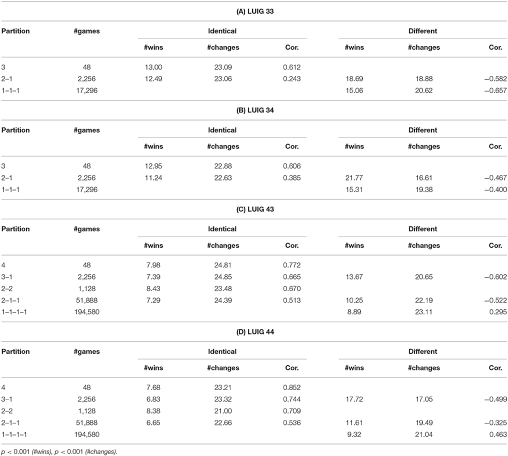
Table 4. Differences of performance with respect to the constitution of players (p-values are from Wilcoxon signed rank test).

There is one point to be addressed; When one reviews Table 4, s/he may notice the difference of Pearson's correlation for the partition 1–1–1–1 of LUIG43 and LUIG44. That is, negative correlations in experimental results whereas positive correlations in computational results. This is because these correlations are obtained from 17,296 (three-person LUIGs) or 194,590 (four-person LUIGs) groups, not from those which were played in the laboratory (16 groups in three-person LUIGs and 12 groups in four-person LUIGs). Hence, if s/he calculates correlations by picking up only the corresponding pairs, the value is −0.820 in LUIG43 and −0.767 in LUIG44 respectively. Likewise, the correlation is −0.755 in LUIG33 and −0.737 in LUIG34 respectively. This means that the computational experiment supported the experimental findings for the groups generated in the laboratory and, at the same time, that the earlier laboratory experiment might have needed more subjects. Instead, the possible reason why the sign of Pearson's correlation is opposite is that the relative frequencies of game outcome in four-person LUIGs were not reproduced, which might stem from the learning of calibrated agents.

Finally, Table 5 shows the difference of the numbers of wins and changes between the types of subjects in each partition of LUIGs. The average values are in these tables and p-values are from Kruskal-Wallis test. The last column of each table explains the results of multiple comparisons if the corresponding pairs have significant differences (5%) and the details are given in the footnote of each panel.

TABLE 5

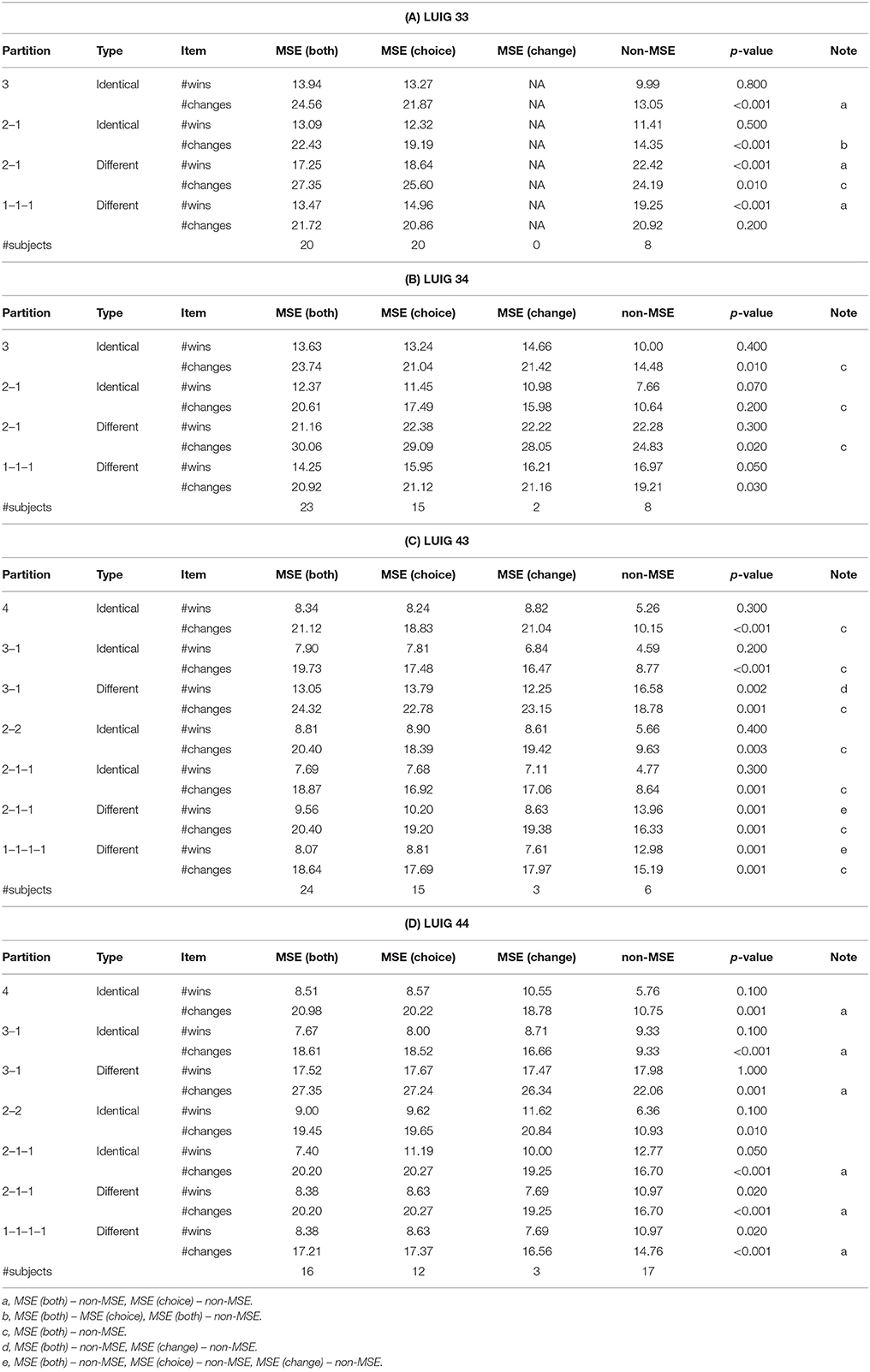
Table 5. Differences between types of subjects with respect to the numbers of wins and changes in computational round robin contest.

When agents are identical in the group, MSE (both) agents seemed to win more than non-MSE agents while they changed more frequently. On the other hand, when the agents are different, non-MSE agents won more than MSE (both) agents by not changing their choices. Since the subjects were all different in every group, one will experimentally and computationally find that sticking behavior is quite effective so long as there are no identical players in small-sized LUIGs.

To summarize, the extent of behavioral heterogeneity may depend on the scale of LUIGs, the number of players in a group and the upper limit. In addition, the observed game outcomes and individual performances depend on the constitutions of agents. In particular, behavioral heterogeneity may improve the chances of win. When there is a mixture of identical agents and different agents, different agents win more than identical agents. However, a full of diversity lessens the winning opportunities for each different agent. With respect to individual performance, the computational experiment shows that keeping on choosing the same number leads the agents to win more, which supports the experimental findings.

4. Discussion

This study computationally examines (1) how the behaviors of subjects are represented, (2) whether the classification of subjects is related to the scale of the game, and (3) what kind of behavioral models are successful in small-sized LUIGs by using the earlier experimental data by Yamada and Hanaki [1]. For these purposes, the behavior of subjects is calibrated and determined among the several typical learning models. Then computational round robin competition including the games where every agent faces not only different agents but also him/herself is pursued. The main findings are as follows: First, the subjects who played not differently from the MSE prediction tended to made use of not only their choices but also the game outcomes meanwhile those who deviated from the MSE prediction took care of only their choices as the complexity of the game increased. Second, when groups consist of different agents which is the case of the earlier laboratory experiment, sticking behavior is quite effective to win LUIGs. Third, when groups consist of different agents like in the earlier laboratory experiment, sticking behavior is quite effective to win.

Since this study deals with the estimated learning models, unlike in Linde et al. [17], there may be better models for some of the behavioral data in laboratory experiment. Hence, as done by Linde et al., it is necessary to conduct another laboratory experiment where subjects are asked to elicit their decisions to play LUIGs. Another future work includes larger-sized experiment to see whether similar behaviors and game dynamics are also observed. This comes form the empirical finding by Östling et al. [4] and Mohlin et al. [18].

Author Contributions

TY built research questions, wrote and ran computer programmings, analyzed the experimental and computational results, and wrote the manuscript.

Conflict of Interest Statement

The author declares that the research was conducted in the absence of any commercial or financial relationships that could be construed as a potential conflict of interest.

Acknowledgments

Financial support from Japan Society for the Promotion of Science (JSPS) Grant-in-Aid for Young Scientists (B) (24710163) and Grant-in-Aid (C) (15K01180), from Canon Europe Foundation under a 2013 Research Fellowship Program, and from JSPS and ANR under the Joint Research Project, Japan – France CHORUS Program, “Behavioural and cognitive foundations for agent-based models (BECOA)” (ANR-11-FRJA-0002) is gratefully acknowledged.

Footnotes

1. ^The list of related work is found in Yamada and Hanaki [1].

2. ^The whole explanation for the experimental design and the mixed-strategy Nash equilibrium in each LUIG are given in Yamada and Hanaki [1].

3. ^Similar learning model in Swedish lottery is proposed by Mohlin et al. [6]. In their model, players using the model pay attention to the numbers around the winning number when they lose. But, since the number of options in LUIGs here is much smaller, it may be possible to take into account the numbers except their chosen number in the same situation. If the players consider only the winning number, the following “naive imitation” model is applied.

4. ^Since there are no information about the winning number at the beginning of the computational experiments, they choose one integer in accordance with the exponential selection rule.

5. ^Level-k thinking in LUIGs chooses a strategy randomly (k = 0), 1 (k: odd), and 2 (k: even).

6. ^“optim” function in R was used for calibration.

7. ^The source code is available upon request.

8. ^Choice criterion means whether the relative frequency of chosen number was different from that in MSE prediction meanwhile change criterion does whether the frequency of changing numbers is different from that in theory.

9. ^The agglomeration method was “ward.D2” in R.

10. ^The resulting dendrograms are given in the appendix.

11. ^The meaning of string “10c” is “When number 1 is chosen and the winning number is 0 (= no-winner), the probability to choose the same number (= 1).” Likewise, the meaning of string “12w” is “When number 1 is chosen and the winning number is 2, the updated probability to choose the winning number.”

Appendix

This section gives the generated dendrograms to classify the calibrated agents in computational round robin contests. The x-axis stands for subject ID (session–subject) and y-axis does the distance between the calibrated agents. The expected decision-making of the “median” agents in each cluster is summarized in Table 2.

References

1. Yamada T, Hanaki N. An experiment on lowest unique integer games. Phys A (2016) 463:88–102. doi: 10.1016/j.physa.2016.06.108

CrossRef Full Text

2. Harris L. Trading and Exchanges: Market Microstructure for Practitioners. New York, NY: Oxford University Press (2003).

Google Scholar

3. Hubbard TP, Paarsch HJ. Auctions. Cambridge, MA: MIT Press (2016).

Google Scholar

4. Östling R, Wang JT, Chou EY, Camerer CF. Testing game theory in the field: swedish LUPI lottery games. Am Econ J Microecon (2011) 3:1–33. doi: 10.1257/mic.3.3.1

CrossRef Full Text

5. Rapoport A, Otsubo H, Kim B, Stein WE. Unique bid auction games. In: Jena Economic Research Paper 2009-005. Jena (2009).

Google Scholar

6. Mohlin E, Östling R, Wang JT. Learning by imitation in games: theory, field, and laboratory. In: Economics Series Working Papers 734, University of Oxford, Department of Economics (2014).

Google Scholar

7. Duffy J. Agent-based models and human subject experiments. In: L Tesfatsion and K Judd, editors. Handbook of Computational Economics, vol. 2. Amsterdam: Elsevier (2006). p. 949–1011.

Google Scholar

8. Chen SH. Varieties of agents in agent-based computational economics: a historical and an interdisciplinary perspective. J Econ Dyn Control (2012) 36:1–25. doi: 10.1016/j.jedc.2011.09.003

CrossRef Full Text | Google Scholar

9. Rochiardi MG, Leombruni R, Contini B. Exploring a new ExpAce: the complementarities between experimental economics and agent-based computational economics. J Soc Complex. (2006) 3:13–22. Available online at: https://papers.ssrn.com/sol3/papers.cfm?abstract_id=883682

10. Giulioni G, D'Orazio P, Bucciarelli E, Silestri M. Building artificial economics: from aggregate data to experimental microstructure. A methodological survey. In: F Amblard, F Miguel, A Blanchet, and B Gaudou, editors. Advances in Artificial Economics. Lecture Notes in Economics and Mathematical Systems, vol. 676. Cham: Springer (2015). p. 69–78.

11. Klingert FMA, Meyer M. Effectively combining experimental economis and multi-agent simulation: suggestions for a procedural integration with an example from prediction markets research. Comput Math Organ Theory (2012) 18:63–90. doi: 10.1007/s10588-011-9098-2

CrossRef Full Text | Google Scholar

12. Boero R, Bravo G, Castellani M, Squazzoni F. Why bother with what others tell you? An experimental data-driven agent-based model. J Artif Soc Soc Simul. (2010) 13:6. doi: 10.18564/jasss.1620

CrossRef Full Text | Google Scholar

13. Colasante A. Selection of the distributional rule as an alternative tool to foster cooperation in a public good game. Phys A (2017) 468:482–92. doi: 10.1016/j.physa.2016.10.076

CrossRef Full Text | Google Scholar

14. Del Forno A, Merlone U. From classroom experiments to computer code. J Artif Soc Soc Simul. (2004) 7. Available online at: http://jasss.soc.surrey.ac.uk/7/3/2.html

Google Scholar

15. Camerer CF. Behavioral Game Theory: Experiments in Strategic Interaction. Princeton, NJ: Princeton University Press (2003).

Google Scholar

16. Erev I, Roth AE. Predicting how people play game: reinforcement learning in experimental games with unique, mixed strategy equilibria. Am Econ Rev. (1998) 88:848–81.

Google Scholar

17. Linde J, Sonnemans J, Tuinstra J. Strategies and evolution in the minority game: a multi-round strategy experiment. Games Econ Behav. (2014) 86:77–95. doi: 10.1016/j.geb.2014.03.001

CrossRef Full Text | Google Scholar

18. Mohlin E, Östling R, Wang JT. Lowest unique bid auctions with population uncertainty. Econ Lett. (2015) 134:53–7. doi: 10.1016/j.econlet.2015.06.009

CrossRef Full Text | Google Scholar