Maximum Probability Reaction Sequences in Stochastic Chemical Kinetic Systems

The detailed behavior of many molecular processes in the cell, such as protein folding, protein complex assembly, and gene regulation, transcription and translation, can often be accurately captured by stochastic chemical kinetic models. We investigate a novel computational problem involving these models – that of finding the most-probable sequence of reactions that connects two or more states of the system observed at different times. We describe an efficient method for computing the probability of a given reaction sequence, but argue that computing most-probable reaction sequences is EXPSPACE-hard. We develop exact (exhaustive) and approximate algorithms for finding most-probable reaction sequences. We evaluate these methods on test problems relating to a recently-proposed stochastic model of folding of the Trp-cage peptide. Our results provide new computational tools for analyzing stochastic chemical models, and demonstrate their utility in illuminating the behavior of real-world systems.

Introduction

Increasingly, we have detailed knowledge about the chemical interactions or transformations in which various biomolecules participate. For example, high-throughput assays such as ChIP-chip or ChIP-seq are rapidly identifying the DNA binding sites of transcription factors (Horak and Snyder, 2002; Valouev et al., 2008). Quantitative tandem mass spectrometry allows us to not only identify protein complexes, but also to study how they form (Gingras et al., 2007; Link et al., 1999). Protein folding simulations identify intra-molecular binding events that define different folding paths (Snow et al., 2002). Real-time fluorescence microscopy allows us to see single molecules moving and interacting (Nie et al., 1995; Sekar and Periasamy, 2003).

When studying such interactions at single-cell or even single-molecule levels, mass-action chemical kinetics can be either misleading or simply inapplicable. In such cases, dynamics are more accurately represented by stochastic chemical kinetic models (SCKMs) (Gardiner, 2004; Van Kampen, 2008). These models define a chemical system in terms of the types of molecules or molecular configurations that are possible, the types of chemical interactions or transformations that may occur, and the state-dependent probabilities with which they occur. The state of the chemical system is given by the number of molecules of each type that are present, hence is discrete, and the state evolves stochastically in continuous time, as described in greater detail below. SCKMs are often used, for example, to model stochastic thermodynamic switching between different configurations of a protein (Marinelli et al., 2009), to model the opening and closing of ion channels (Ball and Rice, 1992), and to study the sources of noise in gene expression (Swain et al., 2002; Thattai and van Oudenaarden, 2001).

Considerable effort has been devoted to various computational problems surrounding SCKMs. For example, computing stationary distributions and computing time-dependent state probabilities given an initial state (usually via the chemical master equation) are two classical and well-studied problems (Van Kampen, 2008). The development of correct and efficient methods for simulating the dynamics of such models is another major area of research (Gibson and Bruck, 2000; Gillespie, 1977). More recently, there have been efforts to learn the parameters or even structure of SCKMs based on time series data (Henderson et al., 2010; Tian et al., 2007). SCKMs, which we define carefully below, can also be viewed as a means for describing continuous-time Markov chains (Anderson, 1991). Thus, many theoretical results and methods from the Markov chain literature also apply to SCKMs, although historically the two communities developed largely separately and have focused on different applications.

We focus on a problem that has received very little attention in the SCKM or continuous-time Markov chain communities: finding most-probable reaction sequences connecting temporally-separated observations of the system. Such problems can arise very naturally – for example, as a means of estimating the behavior of a molecular system between experimental observations, or for extracting “prototypical” behaviors connecting different endpoints. For discrete-time stochastic models, such as Markov chains or hidden Markov models, similar trajectory inference problems are of enormous importance, with applications in areas such as path planning, speech recognition, error correction, robot navigation, DNA sequence analysis, user categorization, etc. Moreover, efficient dynamic programming algorithms can be used to find most-probable system trajectories (Bertsekas, 1995; Rabiner, 1989). For SCKMs, there has been work on finding most-probable trajectories in the case of large system sizes, where the SCKM dynamics can be approximated by a stochastic differential equation (Dykman et al., 1994; Liu, 2008). However, we know of no previous work on finding most-probable trajectories in which the continuous-time and discrete-state nature of the SCKM is retained – a distinction that is crucial in settings where molecule counts are very small, including binary presence/absence situations such as the binding state of a gene’s promoter region or the folding state of an individual protein molecule.

We expect that solutions to trajectory inference problems for SCKMs will have widespread utility. For example, towards the end of this paper, we demonstrate this possibility by analyzing an SCKM describing the stochastic folding of the Trp-cage peptide. Other potential applications include finding most-probable sequences of transcription factor binding and interaction leading to gene activation, sequences of protein complex assembly, or sequences of nucleic acid polymer folding. Maximum probability reaction sequences are, of course, only one aspect of the stochastic dynamics of a chemical system. For systems in which the most-probable trajectory is much more probable than the alternatives, or when other probable trajectories are “similar” to the most-probable one, then the most-probable trajectory is representative of the dynamics as a whole. However, if there are many alternative trajectories with similar probability, including possibly quite different end states, then looking at only the single most-probable trajectory may be misleading. There are well-established methods for computing transient and stationary probability distributions over the state space (Van Kampen, 2008), and for performing stochastic simulations of chemical systems (Gillespie, 1977). These provide alternative views of system behavior which are not sensitive to issues of the uniqueness or representativeness of maximum probability trajectories. However, transient or stationary distributions do not include trajectory-based information, such as which states follow which other ones. Stochastic simulations, although they include trajectory-based information, are based on random sampling rather than exact calculations. Thus, maximum probability trajectories provide a novel and potentially useful form of information for understanding stochastic chemical systems, and one that is complementary to other computational approaches.

It turns out that trajectory inference for SCKMs is not so readily or elegantly solvable as it is for discrete-time models (Markov chains or hidden Markov models) or for stochastic differential equation models. We show that the probability of a particular trajectory can be evaluated in polynomial time. However, results from the study of Petri nets tell us that finding most-probable trajectories is at least EXPSPACE-hard in general. Nonetheless, we develop a correct exhaustive search method that is sufficient to answer questions in a peptide folding domain. We also propose and evaluate several heuristic optimization strategies on a hard optimization instance from the peptide domain. Our work thus establishes baseline expectations and algorithms for what we believe will turn out to be an important computational problem in analyzing SCKMs and in making inferences based on observational data.

Results and Discussion

Stochastic Chemical Kinetic Models and Problem Statement

An SCKM is a stochastic, continuous-time, discrete-state model of the dynamics of a chemical system. It is specified in terms of a finite set of chemical reactions that may take place between a finite set of chemical species, or types of molecules. In the standard interpretation, one assumes that the molecules are contained in a bounded, well-mixed, fixed-volume, constant-temperature space (Van Kampen, 2008). Extensions to modeling spatial inhomogeneity or temporal variation in parameters are possible (Andrews and Bray, 2004; Gibson and Bruck, 2000; Shahrezaei et al., 2008), but we do not consider them here.

Let there be N chemical species and M chemical reactions that may take place between them. Let ℕ = {0, 1, 2,…}. The state of the system at any time is given by the number of molecules of each species, X = (X₁,…,X_N) ∈ ℕ^N. Reaction i consumes C_ij molecules of species j (the reactants) and produces D_ij molecules of species j (the products). Reaction i can occur in state X only if there are sufficient reactants to match those consumed, in which case we say the reaction is valid in that state. If it occurs, then the resulting state is

While the effects of a reaction occurring are deterministic, which reactions occur and when they occur are both stochastic. The propensity of reaction i to occur in state X is

where r_i is the kinetic rate constant associated to reaction i. Let λ(X) = Σ_iλ_i(X) be the total propensity of the reactions in state X. Then, the time until the next reaction is exponentially distributed with parameter λ(X), and, independently of the reaction time, reaction i is the next one to occur with probability λ_i(X)/λ(X). The only exception to these rules is when λ(X) = 0, in which case no reactions can occur, and the system stays in state X forever.

In a given amount of time t, there is no strict limit on the number of reactions that may occur. However, each possible sequence of reactions occurs with some probability. The computational problem we study is: given an initial state X₀, a final time t > 0, and a non-empty target set of states 𝕏, find the/a most-probable sequence of valid reactions that brings the system from X₀ to any state in 𝕏 in time t. In the special case that 𝕏 = ℕ^N, one is simply asking for the most-probable reaction sequence to occur over time t, starting from X₀.

The Probability of a Reaction Sequence is Computable in Polynomial Time

Before we address the problem of finding most-probable reaction sequences, we consider how to compute the probability of a particular reaction sequence. This problem is more involved than one might think, though it can be solved in polynomial time¹. Consider a reaction sequence R₁,…,R_k which, from initial state X₀ produces successive states X₁,…,X_K. Let t₀,…,t_K be the random waiting times spent in each state before the next reaction occurs. The probability of the reaction sequence R₁,…,R_K occurring in time t from state X₀ depends on three events: (i) each reaction must be selected among the alternatives, (ii) the reactions must complete by time t, and (iii) no reaction can occur in state X_K until after time t. We can write this as

The first term is easy to compute. The second term concerns sums of exponentially distributed random variables – that is, hypoexponential distributions. In two special cases, there are simple analytical formulae for the densities of such sums. When all the λ(X_i) are equal to a common λ, then the sum of the first K times follows the Erlang distribution.

If all the λ(X_i) are distinct, then the sum of the first K times follows a different distribution.

In either case, the desired probability can then be obtained by computing the convolution:

where . However, as we will see, we commonly encounter situations in which some of the λ(X_i) are the same and some are different, in which case there is no convenient, explicit formula.

We propose a general, polynomial-time approach to computing the probability based on standard transient-distribution calculations from the theory of continuous-time Markov chains. As shown in Figure 1, our strategy is to imagine a continuous-time Markov chain in which each step along the reaction path is one state, and the exponential waiting times in each state are the same as in the corresponding states of the SCKM. In essence, we strip away any alternative reaction paths that might be followed. If we assume that the chain starts in state X₀, then the probability that the chain is in state X_K at time t is precisely the probability that all K reactions of the SCKM complete in time t, but no other reactions occur afterward. Let ρ(t) denote the probability distribution over states of the continuous-time chain at time t. With Q being the matrix shown in Figure 1C, the forward Chapman–Kolmogorov equation states that ρ(t) obeys the linear differential equation (d/dt)ρ = Qρ. The solution to this equation is ρ(t) = e^Qt ρ(0). The matrix exponential, e^Qt, can be computed in a polynomial number of operations (e.g., by converting Qt to Jordan normal form, in which matrix exponentiation is easy). Evaluating the next-to-last component of ρ(t) gives us the second term in Eq. 2, and thus the entire probability of the reaction sequence, in polynomial time. Such a direct approach to computing transient distributions is not generally followed in the SCKM literature because an SCKM can in general have a very large or even countably infinite number of states, leading to an intractably large matrix Q. In the present use, however, we are concerned with only the states along a particular reaction path, so that the computation is tractable. See Materials and Methods for details of our implementation.

FIGURE 1

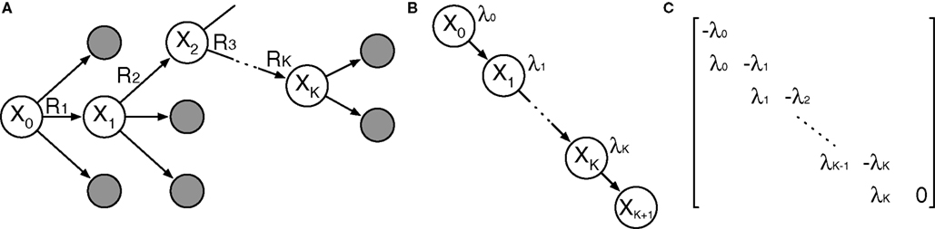
Figure 1. Outline of proposed strategy for computing the probability that a reaction sequence completes in a given amount of time. (A) The reaction sequence picks out a sequence of states starting from X₀. (B) A continuous-time Markov chain describing the timing of transitions along that sequence of states. The waiting time in state X_i is exponentially distributed with parameter λ_i = λ(X_i). (C) The rate matrix for the chain shown in (B).

Finding Most-Probable Reaction Sequences is Computationally Hard

Because the state space, ℕ^N, is countably infinite, it should be no surprise that it is difficult to find a most-probable reaction sequence leading to 𝕏. Indeed, results regarding Petri nets tell us that even establishing the reachability of 𝕏 from X₀ is computationally difficult. Although they have come into much more general use, Petri nets originated as a mean for describing chemical systems (Petri and Reisig, 2008). They have states (species) with markings (molecule counts) and transformations (reactions) which subtract markings from some states and add markings to other states (consume reactants, and produce products). An SCKM is a particular kind of stochastic Petri net, by virtue of its special probabilistic rules for the timing and selection of reactions. The reachability question for general Petri nets, which means finding a sequence of transformations leading from one marking of the states to a different marking of the states, is decidable and EXPSPACE-hard (Esparza and Nielsen, 1994). Various restrictions on Petri nets can reduce the complexity of reachability questions. For example, if markings are restricted to being binary (each molecular species is either present or absent), then the problem is PSPACE-complete (see Esparza and Nielsen, 1994 for more). These results immediately imply similar hardness results for our SCKM problem, because finding a most-probable reaction sequence from X₀ to 𝕏 requires determining whether there is any such reaction sequence at all. More formally, for any Petri net reachability problem, we can pose the decision problem: consider an SCKM with species and reactions corresponding to the states and transitions of the Petri net, let all reaction rates be r_i = 1, let X₀ correspond to the initial marking of the Petri net, and let 𝕏 be a singleton set corresponding to the final marking of the Petri net; does there exist a sequence of valid reactions bringing the SCKM from X₀ to 𝕏 with probability ≥0. Clearly, reachability is true for the Petri net problem if and only if the desired reaction sequence exists for the SCKM (regardless of its probability, as long as the sequence is valid).

Correct Exhaustive Search for the Most-Probable Reaction Sequence

Having established that efficient identification of the most-probable reaction sequence is impossible in general, we next propose an exhaustive approach based on best-first search. Our procedure is “correct” in the sense that if it terminates and returns a reaction sequence, then that sequence is guaranteed to be a maximum probability sequence. Moreover, we establish conditions, which turn out to be readily satisfied in practice, that ensure termination of the search procedure. Thus, when these conditions are met, the algorithm is guaranteed to terminate and return a maximum probability reaction sequence.

Recall that the best-first search procedure maintains a priority queue of partial solutions to the optimization problem (the search frontier), which it repeatedly expands until identifying the optimal solution (Russell and Norvig, 1995). In the present context, a partial solution is any valid reaction sequence beginning in state X₀, whether or not a state in the target set 𝕏 is the result of the reaction sequence. We propose to prioritize a reaction sequence ℛ = (R₁,…,R_K) resulting in state sequence X₀,…,X_K by

where the t_i are the random waiting times in the states X_i. Comparing to Eq. 2, we have dropped the requirement that no other reactions happen before time t. Indeed, Eq. 6 is the probability that ℛ or any extension of that sequence occur in time t. As a consequence, the priority assigned to the sequence is an upper bound on the actual probability of ℛ occurring (Eq. 2), as well as on the actual probability of any extension of the sequence.

Now, the best-first search operates as follows. At all times, the procedure keeps track of the most-probable reaction sequence ℛ* from X₀ to 𝕏 found so far, if any. Let P(ℛ*) denote the probability of that sequence. If no such solution has been found so far, then we write ℛ* = undef. The search is initialized by placing the empty reaction sequence, ℛ = ∅, on the priority queue with priority 1. At each iteration of the search, the highest-priority reaction sequence ℛ is removed from the queue, its priority pri(ℛ) defined by Eq. 6. ℛ is processed according to the following steps. (See Materials and Methods for more detailed pseudocode).

1. If ℛ* ≠ undef and pri(ℛ) ≤ P(ℛ*), then terminate the search, returning ℛ* as the solution.

2. If ℛ results in a state in 𝕏, then compute the exact probability of that reaction sequence, P(ℛ). If P(ℛ) > P(ℛ*), then set ℛ* equal to ℛ.

3. Add every possible single-reaction extension of ℛ to the priority queue.

If the algorithm terminates in line 1, then the following reasoning establishes the correctness of the solution returned. First, if the search finds a solution of probability P(ℛ*), and the highest-priority partial solution in the queue has priority pri(ℛ) < P(ℛ*), then neither that partial solution nor any extension of it can have probability higher than P(ℛ*). This is true because of how we have chosen the priority function. Moreover, all other partial solutions in the queue have priority no higher than P(ℛ), and so neither they nor any extensions of them can have probability higher than P(ℛ*). This establishes the correctness of the algorithm.

Whether or not the algorithm terminates at all is another question. If there are infinitely many possible reaction sequences, but none leads to the target set 𝕏, then the algorithm does not terminate. If 𝕏 is reachable, then the only way the algorithm can fail to terminate is if the search explores arbitrarily long reaction sequences without ever triggering the termination condition. From Eq. 6, for this to happen requires an infinite reaction sequence for which converges rapidly to one and for which P(t₀ + t₁ + t₂ +…≤ t) > 0 is not too small. The latter condition implies that λ(X_i) → +∞, which, considering Eq. 1, implies that the number of molecules of at least one of the species must escape to infinity in finite time. One can write down SCKMs with this property. For example, the SCKM with a single species A, and a single-reaction rule 2A → 3A, has finite probability of generating infinitely many A’s over any finite time interval. Such SCKMs are obviously physically impossible, let alone biologically realistic, so we do not consider this a great concern. As long as reachability and probability one finiteness of all molecular counts over time t can be established, both of which are often straightforward in practice, then the search will terminate.

An Analysis of Trp-Cage Folding

To demonstrate the potential utility of the problem we have formulated, we consider a recently-proposed model of Trp-cage folding (Marinelli et al., 2009). Trp-cage is a synthetic peptide of 20 amino acids. Marinelli et al. (2009) used molecular dynamics computations to estimate the major configurations in which the peptide can reside, and the transitions between those configurations. They proposed the five-state model shown in Figure 2A. This model can be analyzed within the framework of SCKMs by equating each possible configuration with a distinct chemical species and the transitions between them as different chemical reactions.

FIGURE 2

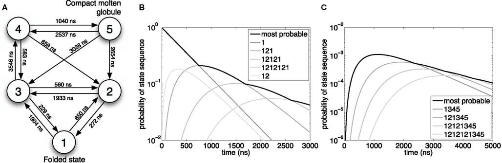
Figure 2. Most probable reaction sequences for a model of Trp-cage folding. (A) High-level model of Trp-cage stochastic folding dynamics from Marinelli et al. (2009). Circles correspond to major configurations, with “1” being the most stable, folded configuration, and “5” being an un/mis-folded configuration that is rarely visited but difficult to escape from. Arcs represent possible transitions and are labeled with the expected time for a transition to occur – the inverse of the kinetic rate constant r_i for that reaction. (B) The probability of the most-probable state sequence, and of several specific state sequences, as a function of time, assuming the peptide begins in state 1 and can end in any state. (C) The probability of the most-probable state sequence, and of several specific state sequences, as a function of time, assuming the peptide begins in state 1 and ends in state 5.

We used best-first search to compute answers to two questions. For the first question, we consider the problem in which the peptide is initially in the folded state, 1, and we ask what is the most-probable sequence of reactions (or equivalently, configurations of the peptide) for varying end times t, allowing for any possible end state. The results are shown in Figure 2B. For short end times, the peptide stays in the folded state the whole time. However, with more time, it becomes more likely for the peptide to switch to state 2 and then back to the folded state. Interestingly, the intermediate possibility of moving to state 2 and still being there at time t is not a most-probable outcome for any t. With even more time, the peptide is most likely to switch back and forth two or more times between state 1 and state 2. Figure 2B also shows the probabilities of these individual state sequences as a function of time.

Figure 2C shows the results of our second analysis, in which we assumed that the peptide starts in the folded state and ends in state 5. At the smallest times, the shortest possible state path, 1 → 3 → 4 → 5, is most-probable. Unlike the previous example, however, this most-probable path has probability approaching zero as t → 0, because it is very unlikely for the peptide to go from the folded state to the molten globule state in so little time. For larger amounts of time, the most-probable path has the peptide flipping between states 1 and 2 before following the 3 → 4 → 5 route to the molten globule state.

As one would expect for exhaustive search, the time complexity increases approximately exponentially with increasing end time and/or optimal solution length. For example, for the second problem, at t = 1000, 2000, 3000, 4000, and 5000 ns, the search either evaluates a candidate solution or evaluates the lower bound (Eq. 6) 210, 787, 2492, 6633, and 15,286 times respectively. The evaluation of solutions or lower bounds is the dominant computational cost in the search.

Probabilistically Correct Search by Stochastic Sampling

Although best-first search can identify optimal solutions, its exponential time complexity encouraged us to look for simpler, heuristic approaches. A simple, non-exhaustive method to search for high-probability reaction sequences is to generate sequences randomly, computing the probability of all those that result in a state in 𝕏, and keeping track of the best solution found. In particular, we propose to generate reaction sequences using Gillespie’s stochastic simulation algorithm (Gillespie, 1977), which generates random realizations of the stochastic dynamics of an SCKM. From start state X₀, Gillespie’s algorithm repeatedly generates a random waiting time until the next reaction and a random next reaction, until reaching the final time t. While simple, this approach is not entirely naive. Of all possible reaction sequences that result in a state in 𝕏, the one with the highest true probability has the greatest chance of being generated. If the highest probability reaction sequence has probability p, then the chance that this approach fails to find it in K random realizations of the dynamics is (1 − p)^K. In the limit as K → +∞, the optimal reaction sequence is found with probability one, and in particular, the probability of not finding the optimal solution decreases exponentially in the number of attempts made. However, the expected number of random samples until the optimal sequence is found is 1/p, which can be quite large when the most-probable path has low probability.

We tested the Gillespie generate-and-test approach on the Trp-Cage domain, using the problem with initial state 1, final state 5, and final time t = 5000 ns. From the best-first search results, we knew the optimal reaction sequence, and we knew its probability p ≈ 1.09 × 10⁻⁴. We allowed the Gillespie approach to generate K = 15,286 trajectories, equal to the number of trajectories scored or lower-bounded by the best-first search. We repeated this procedure 100 independent times. The results are shown in Figure 3. Figure 3A shows that as more and more trajectories are generated, an increasing fraction of the 100 runs found the optimal solution. By the end, 78 of the runs had done so, consistent with the predicted fraction of 1 − (1 − p)^K ≈ 0.81. Figure 3B shows the geometric average of the probabilities of the best solutions found by the 100 runs as more trajectories are generated. Although it is not obvious from the figure, many runs find alternative solutions before identifying the optimal one – some only a little worse, and some startlingly worse, with probabilities of 10⁻¹⁰ or smaller. After 15,286 trajectories, the worst of the 100 runs had found a best state sequence of 1212121212121345, which has probability ≈4.61 × 10⁻⁵.

FIGURE 3

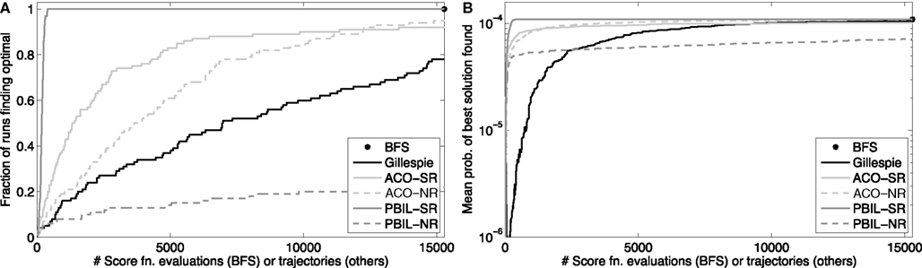
Figure 3. Heuristic optimization results on the peptide problem with initial state 1, final state 5, and final time t = 5000 ns. “BFS” refers to best-first search, “Gillespie” to the generate-and-test approach using the Gillespie algorithm, “ACO” to ant colony optimization, and “PBIL” to population-based incremental learning. The suffix “-SR” denotes the SR matrix representation for ACO or PBIL, whereas “-NR” denotes the number-of-reactions/reaction matrix representation. (A) The fraction of 100 independent runs discovering the optimal solution as a function of the number of sample trajectories. (B) The geometric mean, across the 100 runs, of the probabilities of the best solutions found as a function of the number of sample trajectories.

Adaptive Generate-and-Test Optimization Approaches

Given the partial success of the Gillespie approach, we decided to try more general heuristic optimization approaches, while staying within the overall generate-and-test scheme. We supposed that information from previously-evaluated reaction sequences could be used to bias the random generation towards better solutions. We tried two approaches, Ant Colony Optimization (ACO) (Dorigo et al., 2006) and Population-Based Incremental Learning (PBIL) (Baluja, 1994). ACO has been applied to protein folding before (Shmygelska and Hoos, 2005), albeit in a rather different problem formulation. Both approaches employ a matrix to summarize the results of previous solution attempts, and to guide the generation of future solutions. We tried two different matrix representations. In our SR representation, the matrix is indexed by states of the system (1–5) and “actions” (1–14, corresponding to the 13 reactions and an “end here” action which ends a reaction sequence at the current state; this action was allowed only in state 5, and of course, other reactions were only allowed from their source states). Intuitively, the entries of the matrix represent an estimate of how good it is to take the action (extending the reaction sequence, or ending it) in the given state. In our number-of-reactions/reactions (NR) representation, the matrix is indexed by the number of reactions so far (0–20) and actions (1–14). Here, the entries represent an estimate of how good it is to choose a next reaction or end the reaction sequence depending on how long the reaction sequence already is. In this representation, if 20 reactions are generated without reaching the target state, the reaction sequence is discarded. ACO updates its matrix after every attempt at generating a solution, whereas PBIL makes a set of attempts and updates its matrix based on the best (and optionally worst) solution(s) found in that set. We used standard implementations and default parameter settings for these algorithms; see Section “Materials and Methods” for details. Our goal was not necessarily to obtain the best possible performance, but rather to test how well off-the-shelf heuristic approaches would perform without any tuning.

The results of 100 independent runs of these two approaches and two representations are shown in Figure 3. With the SR representation, both ACO and PBIL significantly outperform the Gillespie approach, both in terms of how many of the runs discovered the optimal solution and in mean solution quality. PBIL was especially successful. All 100 runs discovered the optimal solution, taking just 183.14 sampled trajectories on average, and 399 for the worst of the 100 runs. Although ACO-NR outperformed Gillespie, PBIL-NR did rather poorly. Only 22 runs of the latter found the optimal solution, although the mean solution score rose quickly early on. These results show that, at least on this problem, heuristic approaches can improve on the performance of both Gillespie and best-first search, by using information from earlier trajectories to guide the generation of new candidate solutions.

Materials and Methods

Computing Reaction Sequence Probabilities

As described above, given an SCKM, an initial state X₀, a reaction sequence R₁,…,R_K, and a final time t, we compute the probability of that reaction sequence as follows. Let X₁,…,X_K be the states that result from the corresponding reactions. First, we compute the propensities of every reaction i in every state X_j, 0 ≤ j ≤ K, along the reaction path, λ_i(X_j). By summing over reactions, this gives us the total propensities in each state, λ(X_j). From these propensities, we straightforwardly compute the first term of Eq. 2. For the second term, we form the matrix Q, as described in Figure 1. We multiply this by t element-wise, to obtain Qt. We then compute the matrix exponential of this using the expm function of matlab. The entry in the first column and next-to-last row of this matrix is the probability that all reactions complete in time t, but no reaction occurs in state X_K.

Best-First Search for a Most-Probable Reaction Sequence

Suppose we are given an SCKM, an initial state X₀, and a target set 𝕏. For our best-first search, we assume access to several helper functions. RSP computes the probability of a particular reaction sequence (Eq. 2). RSPUB computes Eq. 6, which is an upper bound on the probability of a reaction sequence as well as any extension of that reaction sequence. EndsInTargetSet tell us whether a given reaction sequence results in a state in 𝕏. Extensions returns a list of all valid one-reaction extensions of a given reaction sequence. We also use a priority queue PQ, which supports enqueue, dequeue, and not-empty functions.

Ant Colony Optimization and Population-Based Incremental Learning Details

Both ant colony optimization (ACO) and population-based incremental learning (PBIL) use a non-negative matrix, M, to summarize the successes and failures of previous attempts at generating solutions to the problem. In the state/reaction (SR) representation, M has 5 rows (corresponding to the five possible states of the system) and 14 columns. The columns correspond to extending a partial solution by one of the 13 possible reactions, though in any given state only a few of these are actually possible, or choosing to end a reaction sequence, which is allowed only if the previous reactions have brought us to the target state. In the number-of-steps/reaction representation (NR), M has 21 rows (corresponding to 0 to 20 reactions having been chosen so far), and 14 columns (which have the same meaning as in the SR representation). Both ACO and PBIL use M to generate candidate solutions in the same way, though the exact method depends on whether the SR or NR representation is used, as shown below. Note that the NRSeq method does not always succeed in generating a reaction path ending at the target state, whereas the SRSeq method keeps going until it chooses “end here” at the target state.

Algorithm 1 Best-first search for optimal reaction sequence
 // Initialization
 RSeq ←∅
 PQ.enqueue(1,RSeq)
 BestRSeq ← undef
 BestProb ← 0
 // Continue search as long as nodes on priority queue
 while PQ.notempty do
  (Priority,RSeq) ← PQ.dequeue
  // If highest-priority node has worse score than a
     solution already found, we're done
  if BestProb ≥ Priority then
     return BestRSeq
  end if
  // If reaction sequence brings us to 𝕏, compute
     probability and record, if appropriate
  if EndsInTargetSet(RSeq) then
      Prob ← RSP(RSeq)
      if Prob > BestProb then
          BestProb ← Prob
          BestRSeq ← RSeq
      end if
  end if
  // Consider all possible extensions of the reaction
     sequence
  for all RSeqExt in Extensions(RSeq) do
    Priority ← RSPUB(RSeqExt)
    PQ.enqueue(Priority,RSeqExt)
  end for
 end while
 return BestRSeq

Algorithm 2 SRSeq: SR method for generating random sample
   reaction sequences
  RSeq ←∅
  KeepGoing ← true
  while KeepGoing do
   i ← the state resulting from RSeq
   J ← the set of reactions possible from state i, and
     the "end here" choice, if i is the target set
   Choose j ∈ J with probability proportional to Mij
   if j = "end here" then
     KeepGoing ← false
   else
     Add j to the end of RSeq
   end if
  end while
  return RSeq

Algorithm 3 NRSeq: NR method for generating random sample
     reaction sequences
  RSeq ←∅
  KeepGoing ← true
  while KeepGoing do
  i ← the state resulting from RSeq
  J ← the set of reactions possible from state i, and
    the "end here" choice, if i is the target set
  Choose j ∈ J with probability proportional to Mij
  if j = "end here" or length(Rseq)=20 then
       KeepGoing ← false
  else
       Add j to the end of RSeq
  end if
 end while
 return RSeq

Ant colony optimization updates its matrix M after every target-reaching reaction sequence is generated and its probability computed. The intuition is that choices leading to higher-probability solutions get bigger increments in the M matrix. Pseudocode for the algorithm is given below. The outermost loop can be done a fixed number of times, or until some other criterion is satisfied. We stopped each run when it had either generated 15,286 candidate reaction paths or it had found the optimal solution, whichever came first. The matrix update depends on a parameter δ, which we take to be 0.1.

Algorithm 4 Ant Colony Optimization (ACO)
  BestRSeq ← undef
  BestProb ← 0
  while not <Termination Condition> do
   // Generate a candidate solution
   RSeq ← SRSeq (or NRSeq)
   // If it's a valid solution, compare with best solution
      and update M
  if RSeq results in a state in 𝕏 then
      Prob ← RSP(RSeq)
      if Prob > BestProb then
          BestProb ← Prob
          BestRSeq ← RSeq
      end if
      for all State- (or step-) reaction pairs (i,j)
          specified by RSeq do
         Mi,j ← (1 −δ) Mi,j − 1/log(Prob)
      end for
  end if
  end while
  return BestRSeq

Algorithm 5 Population Based Incremental Learning (PBIL)
  BestRSeq ← undef
  BestProb ← 0
  while not <Termination Condition> do
    Generate PopSize candidate solutions by SRSeq (or
    NRSeq)
    Compute the probabilities of any valid solutions
    generated
    if at least one valid solution was generated then
       RSeq ← the highest-probability valid solution
       Prob ← RSP(RSeq)
       // Compare against best solution so far
       if Prob > BestProb then
          BestProb ← Prob
          BestRSeq ← RSeq
       end if
       // Update matrix M
       for all State- (or step-) reaction pairs (i,j)
           specified by RSeq do
           Mi,j ← (1 - δ) Mi,j +δ
           Mi,j ← (1 - δ)Mi,jδ for all j' ≠ j
         end for
      end if
      // "Mutate" the matrix M
      for all State- (or step-) reaction pairs (i,j) do
          With probability ρ, perform the following update,
          where r is a uniform random variable on [0, 1]:
          Mi,j ← Mi,j + μ× r
      end for
      Normalize rows of M so they sum to one
    end while

Population-based incremental learning takes a more complicated approPBIL takes a more complicated approach to updating M. It repeatedly generates a batch of PopSize = 10 candidate solutions using either the SR or NR method. It checks whether each solution is valid in the sense of leading to the target set. It finds the best of those, and increases the probabilities of the choices that led to it, decreasing the probabilities of the other choices. Then, it randomizes the matrix M by a small amount. The rows of the matrix M are maintained to sum to one, so that they can be interpreted as probabilities. The algorithm depends on a learning rate parameter δ = 0.1, a mutation probability ρ = 0.02, and a mutation shift μ = 0.05, all recommended default values (Baluja, 1994).

Conclusion

We have proposed a novel computational problem, that of finding most-probable reaction sequences for SCKMs, and studied its solution. We believe that this problem is relevant to molecular biology now, and will grow in relevance as we obtain better characterizations of the stochastic chemical behavior of biomolecules and biomolecular networks. We have demonstrated the potential utility of the problem formulation by analyzing a stochastic model of peptide folding. Many other applications can be envisaged. For example, one might, in a similar fashion, study most-probable sequences of transcription factor-DNA binding events that lead to gene activation or most-probable sequences of protein-protein interaction events in protein complex assembly.

We showed that computing the probability of an individual reaction sequence can be done in polynomial time, but that finding most-probable reaction sequences is computationally intractable in general. In essence, this is because the reachability question itself is hard. It is an open question whether our SCKM problem is any harder than the reachability problem. Conversely, if we can establish reachability by other means, as is often possible in practical applications, does the optimization problem become any easier? Even in the case that the reachable state space is polynomial in the size of the problem description, we have not been able to derive an efficient algorithm for finding optimal reaction sequences. The complex, non-linear form of the reaction sequence probability (see Eq. 4 especially), defies convenient decomposition. The probability of a particular reaction sequence is non-monotone in t, while, for fixed t, adding extra reactions to the end of a sequence may either increase or decrease its probability. We conjecture that finding most-probable reaction sequences is intractable even if reachability of 𝕏 is guaranteed and the reachable state space is polynomial in size, but this remains to be determined definitively.

We proposed a correct exhaustive search method for finding most-probable reaction sequences, and demonstrated its use in analyzing folding behavior in a high-level model of Trp-Cage molecular dynamics. Although the focus of this paper was on establishing basic hardness results and a first correct algorithm, we also evaluated several heuristic approaches to solving the problem. The results on the peptide folding problem indicate that heuristics have the potential to outperform exhaustive search, with one form of PBIL doing particularly well. However, no general conclusions can be drawn without a more thorough empirical study. We have no doubt that improved heuristic solution methods can be developed, and we are actively working on doing so. Another important avenue for further research is to look at more sophisticated types of queries. For example, one may be interested in most-probable folding paths of a protein that avoid certain states or interactions – such as mis-folded states that may be associated with diseases (Selkoe, 2004) or interactions that may be the target of pharmaceutical interventions. More generally, one can imagine marrying temporal logics with SCKMs (similar to Chabrier-Rivier et al., 2004) to ask a host of important questions about the stochastic behavior of biomolecular systems.

Conflict of Interest Statement

The authors declare that the research was conducted in the absence of any commercial or financial relationships that could be construed as a potential conflict of interest.

Acknowledgments

This work was supported in part by grants from the National Sciences and Engineering Research Council of Canada and The Ottawa Hospital Research Institute.

Footnote

1. ^This is a slight bending of the truth. The computation requires evaluation of the exponential function, which, being a transcendental function, can only be done to some desired accuracy (Macintyre and Wilkie, 1996; Weispfenning, 2000). If we treat exponentiation as a unit-time, or at least poly-time, operation, then the claim is true as stated.

References

Anderson, W. J. (1991). Continuous-Time Markov Chains: An Applications-Oriented Approach. New York: Springer-Verlag.

Andrews, S. S., and Bray, D. (2004). Stochastic simulation of chemical reactions with spatial resolution and single molecule detail. Phys. Biol. 1, 137–151.

Pubmed Abstract | Pubmed Full Text | CrossRef Full Text

Ball, F. G., and Rice, J. A. (1992). Stochastic models for ion channels: introduction and bibliography. Math. Biosci. 112, 189.

Pubmed Abstract | Pubmed Full Text | CrossRef Full Text

Baluja, S. (1994). Population-Based Incremental Learning. Pittsburgh: School of Computer Science, Carnegie-Mellon University. Technical Report Number CMU-CS-94-163.

Bertsekas, D. P. (1995). Dynamic Programming and Optimal Control. Athena, MA: Scientific Belmont.

Chabrier-Rivier, N., Chiaverini, M., Danos, V., Fages, F., and Schächter, V. (2004). Modeling and querying biomolecular interaction networks. Theor. Comp. Sci. 325, 25–44.

CrossRef Full Text

Dorigo, M., Birattari, M., and Stutzle, T. (2006). Ant colony optimization. IEEE Comput. Intell. Mag. 1, 28–39.

Dykman, M. I., Mori, E., Ross, J., and Hunt, P. M. (1994). Large fluctuations and optimal paths in chemical kinetics. J. Chem. Phys. 100, 5735–5750.

CrossRef Full Text

Esparza, J., and Nielsen, M. (1994). Decidability issues for petri nets – a survey. J. Inf. Process. Cybern. 30, 143–160.

Gardiner, C. W. (2004). Handbook of Stochastic Methods: For Physics, Chemistry and the Natural Sciences. New York: Springer-Verlag.

Gibson, M. A., and Bruck, J. (2000). Efficient exact stochastic simulation of chemical systems with many species and many channels. J. Phys. Chem. A 104, 1876–1889.

CrossRef Full Text

Gillespie, D. T. (1977). Exact stochastic simulation of coupled chemical reactions. J. Phys. Chem. 81, 2340–2361.

CrossRef Full Text

Gingras, A. C., Gstaiger, M., Raught, B., and Aebersold, R. (2007). Analysis of protein complexes using mass spectrometry. Nat. Rev. Mol. Cell Biol. 8, 645–654.

Pubmed Abstract | Pubmed Full Text | CrossRef Full Text

Henderson, D. A., Boys, R. J., and Wilkinson, D. J. (2010). Bayesian calibration of a stochastic kinetic computer model using multiple data sources. Biometrics 66, 249–256.

Pubmed Abstract | Pubmed Full Text | CrossRef Full Text

Horak, C. E., and Snyder, M. (2002). ChIP-chip: a genomic approach for identifying transcription factor binding sites. Meth. Enzymol. 350, 469–483.

Pubmed Abstract | Pubmed Full Text | CrossRef Full Text

Link, A. J., Eng, J., Schieltz, D. M., Carmack, E., Mize, G. J., Morris, D. R., Garvik, B. M., and Yates, J. R. III. (1999). Direct analysis of protein complexes using mass spectrometry. Nat. Biotechnol. 17, 676–682.

Pubmed Abstract | Pubmed Full Text | CrossRef Full Text

Liu, D. (2008). A numerical scheme for optimal transition paths of stochastic chemical kinetic systems. J. Comput. Phys. 227, 8672–8684.

CrossRef Full Text

Macintyre, A., and Wilkie, A. J. (1996). On the decidability of the real exponential field. Kreiseliana: about and around Georg Kreisel. Wellesley: Peters, 441–467.

Marinelli, F., Pietrucci, F., Laio, A., and Piana, S. (2009). A kinetic model of trp-cage folding from multiple biased molecular dynamics simulations. PLoS Comput. Biol. 5, e1000452. doi: 10.1371/journal.pcbi.1000452.

Pubmed Abstract | Pubmed Full Text | CrossRef Full Text

Nie, S., Chiu, D. T., and Zare, R. N. (1995). Real-time detection of single molecules in solution by confocal fluorescence microscopy. Anal. Chem. 67, 2849–2857.

CrossRef Full Text

Petri, C. A., and Reisig, W. (2008). Petri net. Scholarpedia 3, 6477.

CrossRef Full Text

Rabiner, L. R. (1989). A tutorial on hidden Markov models and selected applications in speech recognition. Proc. IEEE 77, 257–286.

CrossRef Full Text

Russell, S., and Norvig, P. (1995). Artificial Intelligence: A Modern Approach. Upper Saddle River, NJ: Prentice Hall.

Sekar, R. B., and Periasamy, A. (2003). Fluorescence resonance energy transfer (FRET) microscopy imaging of live cell protein localizations. J. Cell Biol. 160, 629–633.

Pubmed Abstract | Pubmed Full Text | CrossRef Full Text

Selkoe, D. J. (2004). Cell biology of protein misfolding: the examples of Alzheimer’s and Parkinson’s diseases. Nat. Cell Biol. 6, 1054–1061.

Pubmed Abstract | Pubmed Full Text | CrossRef Full Text

Shahrezaei, V., Ollivier, J. F., and Swain, P. S. (2008). Colored extrinsic fluctuations and stochastic gene expression. Mol. Syst. Biol. 4, 196.

Pubmed Abstract | Pubmed Full Text | CrossRef Full Text

Shmygelska, A., and Hoos, H. H. (2005). An ant colony optimisation algorithm for the 2D and 3D hydrophobic polar protein folding problem. BMC Bioinformatics 6, 30. doi: 10.1186/1471-2105-6-30.

Pubmed Abstract | Pubmed Full Text | CrossRef Full Text

Snow, C. D., Nguyen, H., Pande, V. S., and Gruebele, M. (2002). Absolute comparison of simulated and experimental protein-folding dynamics. Nature 420, 102–106.

Pubmed Abstract | Pubmed Full Text | CrossRef Full Text

Swain, P. S., Elowitz, M. B., and Siggia, E. D. (2002). Intrinsic and extrinsic contributions to stochasticity in gene expression. Proc. Natl. Acad. Sci. U.S.A. 99, 12795–12800.

Pubmed Abstract | Pubmed Full Text | CrossRef Full Text

Thattai, M., and van Oudenaarden, A. (2001). Intrinsic noise in gene regulatory networks. Proc. Natl. Acad. Sci. U.S.A. 98, 8614–8619.

Pubmed Abstract | Pubmed Full Text | CrossRef Full Text

Tian, T., Xu, S., Gao, J., and Burrage, K. (2007). Simulated maximum likelihood method for estimating kinetic rates in gene expression. Bioinformatics 23, 84.

Pubmed Abstract | Pubmed Full Text | CrossRef Full Text

Valouev, A., Johnson, D. S., Sundquist, A., Medina, C., Anton, E., Batzoglou, S., Myers, R. M., and Sidow, A. (2008). Genome-wide analysis of transcription factor binding sites based on ChIP-Seq data. Nat. Methods 5, 829–834.

Pubmed Abstract | Pubmed Full Text | CrossRef Full Text

Van Kampen, N. G. (2008). Stochastic Processes in Physics and Chemistry. New York: Elsevier.

Weispfenning, V. (2000). “Deciding linear-transcendental problems,” in Computer Algebra in Scientific Computing: CASC 2000: Proceedings of the Third Workshop on Computer Algebra in Scientific Computing, October 5–9 (Samarkand: Springer Verlag), 423.