Physiological Environment Induces Quick Response – Slow Exhaustion Reactions

In vivo environments are highly crowded and inhomogeneous, which may affect reaction processes in cells. In this study we examined the effects of intracellular crowding and an inhomogeneity on the behavior of in vivo reactions by calculating the spectral dimension (d_s), which can be translated into the reaction rate function. We compared estimates of anomaly parameters obtained from fluorescence correlation spectroscopy (FCS) data with fractal dimensions derived from transmission electron microscopy (TEM) image analysis. FCS analysis indicated that the anomalous property was linked to physiological structure. Subsequent TEM analysis provided an in vivo illustration; soluble molecules likely percolate between intracellular clusters, which are constructed in a self-organizing manner. We estimated a cytoplasmic spectral dimension d_s to be 1.39 ± 0.084. This result suggests that in vivo reactions initially run faster than the same reactions in a homogeneous space; this conclusion is consistent with the anomalous character indicated by FCS analysis. We further showed that these results were compatible with our Monte-Carlo simulation in which the anomalous behavior of mobile molecules correlates with the intracellular environment, leading to description as a percolation cluster, as demonstrated using TEM analysis. We confirmed by the simulation that the above-mentioned in vivo like properties are different from those of homogeneously concentrated environments. Additionally, simulation results indicated that crowding level of an environment might affect diffusion rate of reactant. Such knowledge of the spatial information enables us to construct realistic models for in vivo diffusion and reaction systems.

1 Introduction

The complex physical structure of cytoplasm has been a long-standing topic of interest (Fulton, 1982). The physiological environment of intracellular biochemical reactants is not one of well-diluted, homogeneous space. This fact contradicts the basic assumption underlying the standard theories for reaction kinetics. The difference may make actual reaction processes deviate from those expected by the theories. If we reconcile the fundamental principle with experimental observations, reaction processes are mainly controlled by the movement of reactants. Consequently, when the environment affects molecular movement, the results would be reflected on the reaction process.

The most basic components that describe reaction kinetics are the concentrations of reactants and kinetic rate constants, which determine the probability of collision between reactants and of state transition of each reactant (Atkins and de Paula, 2006; Jackson, 2006).

Physiological events consist of quick responses in a molecular reaction level to environmental changes; i.e., a cell needs to store a portion of reaction species in a reaction environment to respond new sequential signals after current signals. This means a cell needs to quickly respond and to prevent exhaustion of reaction sources at the same time. Classical kinetic models which consist of the molecular concentration and constants fit well to in vitro reaction processes. However, it is too slow at the beginning of a reaction, or if we force to react quickly, the reaction system exhausts the entire reaction source in an early timing of a reaction process. Also, if we choose specific models such as Hill equation, Michaelis–Menten kinetics, etc., we can fit the equations to the shape of the curve of in vivo reaction data; however, the case we can find a satisfactory reason to adopt those equations is still rare even after a century of their development. Our results of this study provide a way to fit the model to in vivo experimental results, also the natural reason to use the model.

The inhomogeneous, crowded feature of the reaction space is the point we should concern to represent in vivo reaction processes precisely. Fractal kinetics has been studied as a candidate to represent in vivo reactions (Berry, 2002; Schnell and Turner, 2004). Kopelman et al. originally built their theory with reactions occurring on fractal structures, later confirmed the reality using a chemical species (naphthalene) on a considerable fractal structure (a filter membrane; Kopelman, 1988, 1991; Parus and Kopelman, 1989). The basic description of fractal kinetics is v = k(t)[A] instead of v = k[A], where v is the reaction rate, k and k(t) are the kinetic constant or function, and [A] is the concentration of a reactant; i.e., the reaction rate depends on t when it occurs on a fractal structure.

A space including fractal structure can be described quantitatively with a parameter named fractal dimension (d_f). The dynamics of particles in the fractal space is expressed by another parameter, which is spectral dimension d_s (Alexander and Orbach, 1982). The spectral dimension d_s is a quantity that can be translated into the kinetic function [k(t)]. Kopelman et al. succeeded to transform d_s into a kinetic function as the exponent in the transformation of the time variable (Kopelman, 1988, 1991; Parus and Kopelman, 1989). Here d_r is the fractal dimension, which has the value 2 in the case of Brownian particle motion in Euclidean space (Einstein, 1905). This means that if a reaction space has fractal structure, we can describe the dynamics of molecules by experimentally derived d_s and can reflect the spatial characteristics into the description. Deriving d_s let us investigate further effect of the intracellular environment on the form of the reaction.

As we mentioned above, the characteristics of reaction space can be quantified with d_f, and the dynamics of a particle or a molecule can be quantified with d_s. Now there remained a question if intracellular environment consists of fractal structures. Aon et al. (2004) performed experiments to analyze the fractality of mitochondria, and cytoskeletal protein-networks. They derived d_f of those organelle but did not use the value directly to calculate d_s.

In our study, we derived the value of d_s directly from our experimental results. We used the relationship between anomaly parameter of diffusion (α) and the above 2D;

It was originally defined by Alexander and Orbach (1982) and Berry (2002). By referring this relationship, we could calculate d_s by the values of α and d_f, which were experimentally obtained by fluorescence correlation spectroscopy (FCS) and transmission electron microscopy (TEM), respectively. Afterward we estimated the reaction kinetics in vivo using the transformed equation from the d_s.

Diffusion coefficient is the parameter to express molecular diffusion. The diffusion represented by α is a specific case which occurs in inhomogeneous space, named anomalous diffusion (Gefen et al., 1983). Anomalous diffusion is described with the mean-square displacement (MSD) as follows;

The case with α = 1 is for the normal diffusion. The case with α < 1 is for anomalous diffusion.

Alexander and Orbach used to express the index governing diffusion. The definition of anomalous diffusion in their description by using MSD is

By comparing Eqs. 2 and 3,

The definition of spectral dimension, in their terminology it is called fracton dimension is

where is fractal dimension (d_f).

Anomalous diffusion was also defined by using a random walker on percolation clusters (Gefen et al., 1983). Percolation theory deals with the number and properties of clusters which are formed as follows (Broadbent and Hammersley, 1957); each site of a very large lattice is occupied randomly with probability p, independent of its neighbors. In other words the group of neighboring occupied sites is the target of percolation theory (Stauffer and Aharony, 1994). When the probability p is over the critical value (p_c), the cluster reaches from a side to the opposite side. This p_c is the threshold to undergo phase transition, such as gelation of polymer sol, and so on. Anomalous diffusion in an inhomogeneous environment is observed when the reaction space is occupied inhomogeneously with obstacles until the relative volume of obstacles reaches close to the threshold. We can obtain each threshold value depending on the shape of the lattice by numerical simulation (Stauffer and Aharony, 1994). The value of p_c for the 3D cube is 0.312. In some of numerical simulation including our model, percolation lattice is used as a simple example of disordered medium. The mass of a cluster M and the linear size of the cluster L keep the relation

When p = 1, the cluster is the same with a regular lattice without disorder. In this case, the time dependency of MSD of the random walker is linear. On the other hand, if the random walker is confined at a specific place, then MSD is settled on a constant. The case between these two extreme cases was named anomalous diffusion by Gefen et al. (1983). The exponent representing the time dependency of MSD equals the anomaly parameter α.

Fluorescence correlation spectroscopy is a technique used to detect single fluorescent signals from molecules in a focal volume. The detected fluctuation can be translated into the diffusion time of the molecules via inverse Fourier transformation (Kohler et al., 2000). We used FCS to estimate α (Eq. 2) by analyzing the measured diffusion time for different pinhole diameters (Rigler et al., 1993).

We controlled intracellular environment with drugs which cause cytoskeletal disorder (for actin disruption: cytochalasin B, for microtubule disruption: colchicine). The aim to treat cells with these drugs is to build a reaction environment, which includes physiological components (such as cytoskeletal proteins, etc.) with original concentration, but the structures of polymers (e.g., actin filaments, microtubule) are not physiological. By using these cells, we could exclude the effect of the molecular concentration, also could avoid using artificial components to build a test environment. As the result, our experiments could investigate purely the meaning of the physiological structures of those filaments.

Transmission electron microscopy image analysis provides a direct check of structural self-similarity. Self-organizing molecules, such as titanium dioxide, and sol–gel powders, etc., are readily seen under TEM. We applied this method to determine the d_f of the intracellular environment using the procedure described by Dobrescu et al. (2004).

Generally, an image obtained by electron microscopy indicates the distribution of electron density of the section. If the electron density is high, the segment in an image appears dark. This means that the density of the electrons captured by cellular components is relatively low at faint-shadowed segment compared with the dark-shadowed segment. Also, there exist many images which investigated intracellular structures by electron microscopy. In those images, organelle, such as nucleus, mitochondria, rough endoplasmic reticulum, zymogen granules, Golgi complex, etc., appear as clear shadows. Based on these facts, we estimated that cytoplasmic diffusion occurs between those components, where thus the faint-shadowed segment.

We produced two different d_fs for two different intracellular areas: one was for the immobile structures (Sd_f), and the other for the mobile area of a solute in a cell (Md_f). Based on the above reasons, we assumed that the black segment in the TEM images consisted of solid structures comprising the non-reactive obstacle. Simultaneously, the non-reactive surface can provide anchorage for small mobile molecules. The faint segment areas in TEM images presumed to be made up of sol proteins, which formed the main reaction chamber for the intracellular reactants.

The objective of analyzing the parameters, two d_fs with α and d_s, was to estimate how the intracellular reaction space affected the reaction process using Md_f and α to calculate d_s, and to estimate environmental organization by comparing Sd_f obtained from TEM with those from the following four numerical models in Table 1, leading to estimation of the underlying mechanism for building the intracellular environment.

TABLE 1

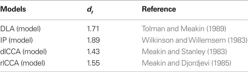
Table 1. Numerical values of d_f from different computational models.

There exist some models in which growing random patterns can evolve into fractal structures. Of particular interest to us are the invasion percolation (IP; Wilkinson and Willemsem, 1983), diffusion-limited aggregation (DLA; Tolman and Meakin, 1989), diffusion-limited cluster–cluster aggregation (dlCCA; Meakin and Stanley, 1983), and reaction-limited CCA (rlCCA) model (Meakin and Djordjevi, 1985), all of which were used to compare our estimated values of d_f with experimental results.

Finally we constructed a numerical model that enables us to verify the consistency of the hypothesis that the intracellular component is built using a kind of self-organization and that the structure provides a percolation cluster-like environment for soluble molecules. We computed α, derived a reaction rate function k(t), and compared experimental results with simulation. Additionally, we computed the MSD of a diffusing molecule to ascertain the effect of the non-reactive obstacles (NRO) in the reaction space.

Our results allow confirmation of the importance of the physiological intracellular structure, and provide new insights into causes of the argued point that a reaction or molecular movement exhibits a quick initial response, and later slows down to avoid exhaustion of the molecular source in physiological environments.

2 Materials and Methods

2.1 Cell Culture

Cell culture reagents for L-929 were obtained from Sigma-Aldrich Corp. (Austria) and EuroClone Group (Austria). Cytochalasin B (CytB) was sourced from Sigma-Aldrich (Austria). Cell culture reagents for 3Y1 cells were obtained from Wako Pure Chemical Industries, Ltd. (Japan). Both cell lines were routinely cultured in Dulbecco’s minimal essential medium (DMEM) supplemented with 10% fetal bovine serum (FBS) in a 5% CO₂ incubator. We obtained both L-929 and 3Y1 cell lines from Japanese Collection of Research Bioresources (JCRB) Cell Bank for use at Keio University.

2.2 Preparation for FCS

Cells (3 × 10⁴ cells/ml) were seeded in eight-well cover glass-bottom LabTek chambered slides (NUNC) and were grown overnight at 37°C. Cells were washed twice with phosphate buffer saline (PBS) at 37°C. For transfection prior to imaging the cells were incubated with a plasmid DNA encoding green fluorescent protein (pEGFP)-LipofectAMINE (Invitrogen) mixture for transfection.

The transfection reagent, LipofectAMINE LTX, was used according to the manufacturer’s instructions. Briefly, we resuspended 3 μg/ml plasmid DNA in 88 μl of serum-free DMEM, and then mixed in 12 μl of LipofectAMINE LTX reagent. After incubation of the mixture of DNA and reagent at room temperature for 30 min, the cells were treated with the after incubated mixture of DNA and reagent. After 48 h of incubation with the DNA, we checked the expression levels of the green fluorescent protein (GFP) fluorescence microscopy.

2.3 FCS Analysis

We performed FCS on GFP-transfected mouse fibroblast, L-929 cells. The FCS measurements were conducted using a confocal spectrofluorimeter (Carl Zeiss-Evotec, Jena, Germany) equipped with an argon (Ar)-laser, a water immersion objective (C-Apochromat 63 W × 1.2 W Korr), an avalanche photodiode (SPCM-CD 3017), and a hardware autocorrelator (ALV 5000, ALV; Langen, Germany). Samples were excited using a 488-nm Ar-laser-line attenuated by optical density filters, and the fluorescence signal was detected through a dichroic mirror with band-pass filters [the excitation filter wavelengths: 477–494 nm (486 central wave length), dichromatic beam splitter wavelength: 508 nm, emission filter wavelength: 517–567 nm (542 central wave length)]. The set pinhole diameter ranged from 25 to 75 μm.

The detected fluctuations were translated into the diffusion time of the molecules via inverse Fourier transformation (Kohler et al., 2000). We estimated α (Eq. 2) by analyzing the measured diffusion time for different pinhole diameters, followed the method of Masuda et al. (2005) and Rigler et al. (1993).

From the expression for free diffusion of Gaussian intensity distribution (G) described in Masuda et al. (2005).

Regarding the second term of Eq. 5, we have

where z is the axial radius, and q = z/w is the structural parameter. Hence, G varies linearly with τ if the second term dominates over the first term.

We tested our model with free diffusion of Rhodamine 6G (R6G). The confocal volume at 45 μm calibrated with R6G was 0.17 μm in the radial and 2.4 μm in the axial dimension. We also tested the assumption that the diffusion time τ_D(=w²/4D) of R6G scales linearly with the pinhole diameter (Hiroi et al., 2011).

For the analysis with colchicine treated cells, we performed FCS with LSM780 and analyzed the data with ZEN 2009 (Carl Zeiss MicroImaging GmbH, Jena, Germany). Calibration methods and the settings of laser, pinhole sizes are the same except the pinhole size for calibration and one of them for anomaly test was changed from 45 or 35 to 34 μm based on the manufacture’s recommended procedures.

2.4 Cytochalasin B Treatment

To test the effect of physiological organization of cytoskeletal proteins, a fraction of L-929 cells was treated with final concentration 2 μM CytB/DMSO for 1 h at 37°C in 5% CO₂ atmosphere prior to FCS analysis. As a negative control 1/100 volume of DMSO/culture medium was prepared. The following steps are identical for both treated and non-treated cells. Under this condition of CytB treatment, we noted that cells adhered to the bottom of the culture chamber.

2.5 Colchicine Treatment

We also performed FCS with colchicine, which is a microtubule inhibitor, treated cells in order to test the effect of physiological organization of cytoskeletal proteins. The other portion of L-929 cells was treated with final concentration 2 μM colchicine/EtOH for 1 h at 37°C in 5% CO₂ atmosphere before FCS analysis. Negative control was performed with 1/100 volume of EtOH/culture medium. The following steps were the same as those used with non-treated cells.

2.6 Transmission Electron Microscopy

We obtained 165 images of rat fibroblast 3Y1 cells and analyzed them by box counting methods.

The source images were the subregion of the images of cytoplasmic region. The cells were collected on the day when the cells reached at the confluent condition in order to obtain the homogeneous population in their cell cycle (G1 to G0 cells).

In preparation for TEM, the cells were fixed with 4% formaldehyde and 2% glutaraldehyde in 0.1 M phosphate buffer (pH 7.4) for 16 h at 4°C, and successively with 1% osmium tetraoxide in 0.1 M phosphate buffer (pH 7.4). The cells were dehydrated in graded ethanol and embedded in epoxy resin. Ultrathin sections (approximately 60 nm thick) were prepared with a diamond knife and were electron-stained with uranyl acetate and lead citrate, and were examined using an electron microscope (H-7650; Hitachi Ltd.).

The parameter d_f was derived from box counting as explained below (Chhabra et al., 1989).

First, the TEM images were binarized into objects and background using the Auto-thresholding function of ImageJ (http://rsbweb.nih.gov/ij/). Briefly, this algorithm computes the average intensity of the pixels at below or above, a particular threshold. It then computes the average of these two values, increments the threshold, and iterates the process until the threshold is larger than the composite average. That is,

A scaling rule for the relation between the count and box size in box counting, assuming that these correspond respectively to details or the number of parts (N) and scale (ε) is given by:

where the limit is found as the slope of the regression line.

We additionally calculated the d_fs of the original images plus Gaussian noise (SD = 0.01 or 0.02), and impulse (salt and pepper) noise (density = 0.05 or 0.1) by using MATLAB. Also, we tested the effect of changing the threshold by taking different ratios between the background and objects. In the original test, the background to object ratio was 0.5. We altered this ratio to 0.4 or 0.6.

2.7 Statistical Tests for d_f Values

We calculated the statistics D of Kolmogorov–Smirnov test, F value of Fisher–Snedecor F-test, and T value of Welch’s test by freely distributed software R (R Development Core Team, 2011).

2.7.1 Kolmogorov–smirnov test for testing normality of the distribution of data population

We confirmed that the two data populations, Md_f and Sd_f were normally distributed by Kolmogorov–Smirnov test.

Null hypothesis H₀ is that the Md_f and Sd_f follow a normal distribution. The alternative hypothesis H_a is the data do not follow a normal distribution.

The test statistics D is defined as

where F in this test is the theoretical cumulative distribution of the distribution being tested. The H₀ is rejected if the test statistics D is greater than the critical value. In our case, the each sample size was 165. Based on the Lilliefors’ 1967 work, the critical value . The calculated D values for Md_f and Sd_f were respectively. We therefore inferred that H₀ was not valid, i.e., these data sets were not distributed normally. We also confirmed the normality of the data distribution by Jarque–Bera test. The result meant that these data sets are not distributed normally as same as the result by Kolmogorov–Smirnov test.

2.7.2 Mann–whitney test

The distributions of both populations departed from normality. Therefore, we performed Mann–Whitney (MW) test to test the following null hypothesis. The null hypothesis H₀ is that two independent samples are drawn from the same population, it means that two samples come from identical population. The alternative hypothesis, H_a is that two independent samples come from different populations.

We computed a statistics U by pooling observations from both samples and sorting them by value. For one of the samples, for each observation, the number of larger-value observations in the alternative sample was counted, and the results summed. This procedure can be repeated for the other sample. When the two values are equal, the half point is added to the statistics. At the same time we calculated the mean of U

together with its SD

We calculated the statistics z as

We used the result of Eq. 6 to derive probability P.

2.7.3 Confidence limits for the mean

The confidential intervals were estimated so that the mean of our experimental d_f values could be compared with that derived from numerically computed d_fs (Wilkinson and Willemsem, 1983; Meakin and Djordjevi, 1985; Tolman and Meakin, 1989; Dobrescu et al., 2004; Table 1). The interval estimation reflects the degree of uncertainty in the derived mean.

Confidence limits are expressed in terms of a confidence coefficient. We applied a 99.0% confidence interval, to be interpreted as follows. We will find a confidence interval between the two stochastic endpoints with probability 0.99, in which we intercept the mean value of the population: the true mean value lies between the endpoints calculated from the sampled mean in 99.0% of cases.

The confidence interval is defined

Therein, signifies the sample mean, s represents the sample SD, N stands for the sample size, a is the desired significance level, and denotes the upper critical value of the t distribution with N − 1 degrees of freedom (DF). The confidence coefficient is 1 − a.

2.7.4 Fisher–snedecor F-test

F-test (Snedecor and Cochran, 1989) was performed for testing equality of 2 SD of the two d_f populations. We performed two-tailed test. Briefly, the F hypothesis test is defined as follows. The null hypothesis H₀ is σ₁ = σ₂, and the alternative hypothesis H_a is σ₁ ≠ σ₂.

The test statistics F is

where N₁ and N₂ are the sample sizes, and are the sample means, and and are the sample variances.

H₀ is rejected when where is the critical value of the t distribution with DF where

In our case, both N₁ = N₂ = 165. When the significance level a = 0.01, the critical value

If T > 2.591, H₀ is rejected, i.e., the two population are not the same.

2.8 Monte-Carlo Simulation of the Reaction Process in Inhomogeneous Crowded Space

We performed a Monte-Carlo simulation to investigate the reaction processes in a pseudo-inhomogeneous 3D space represented by a reaction space randomly interspersed with NRO.

The simulation space is a 50 × 50 × 50 cubic lattice with periodic boundary conditions. The reaction simulated in our model is A + A → A. The location of each reactant at a given time step is assigned randomly. If the chosen lattice site was previously empty, the reactant fills the site; if the site was occupied by a non-reactive obstacle, a new position is randomly allocated for the reactant; if a reactant A1 moves to a site which has been occupied by the other reactant A2, A1 remains at the lattice site and A2 is obliterated. The simulator is implemented in C++ programming language.

We tested another spatial condition by arranging the same volume of NRO as they form one big cube in the reaction space, and analyzed the effect of the shape of NRO.

The number of time steps was 1,000, 10,000, or 40,000. The initial amount of the reactant was 1,000. The spatial conditions defined by the relative volume of NRO were changed at 10% increments from 10 to 70%. Simulations were performed 100,000 times for each condition.

3 Results

In this study, two separate biological experiments were conducted using mammalian cell lines and the results compared with the output of a single numerical model analysis. Experiments yielded values of the anomaly parameter α and fractal dimensions Sd_f and Md_f. Numerical simulations yielded an independent estimate of α, and also allowed us to observe the time course of in silico reactions. We compared the reaction form predicted by k(t), derived from

and produced by the simulation. We also simulated MSD for each different condition of the reaction space.

3.1 Anomaly Parameters Analyzed Using FCS

3.1.1 The case of normal cells

Fluorescence correlation spectroscopy analyses were performed to infer the molecular dynamics in vivo. Reportedly, spherical proteins diffuse anomalously inside the cell (Weiss et al., 2004; Malchus and Weiss, 2010). We determined the anomaly parameters of GFP in the cytoplasmic region.

We used GFP-transfected mouse fibroblast cells, L-929, for the FCS analysis.

The confocal volume at 45 μm pinhole diameter calibrated with R6G was 0.17 μm in the radial and 2.4 μm in the axial dimension. We also confirmed the linearity of the relationship between diffusion time τ_D(=w²/4D) of R6G and pinhole diameter (Hiroi et al., 2011). Based on these calibration results, we evaluated the microscope system as suitable for further experiments.

The calculated α based on the 160 FCS data of GFP diffusion in cytoplasm was 0.768 ± 0.14 (Figure 1B). This result is compatible with the previously reported results that GFP shows anomalous diffusion in cytoplasm (Weiss et al., 2004).

FIGURE 1

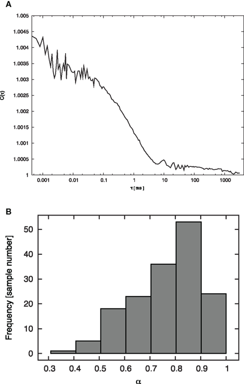
Figure 1. Estimated anomaly parameters based on 160 FCS data. (A) Relationship between diffusion time t and auto-correlation function C(τ). This sample was obtained using a 45-μm diameter pinhole. Calibration was undertaken with R6G at four settings of the pinhole diameter (25, 35, 45, 75 μm; Hiroi et al., 2011). (B) The histogram indicates the distribution of the anomaly parameter α obtained from 160 measurements with GFP in the cytoplasmic region.

3.1.2 Effect of cytochalasin B treatment

We verified that the anomaly characteristics depend on the physiological intracellular structure by performing the same analysis on CytB-treated cells. CytB is a drug that disorders the actin polymer. Treatment with CytB breaks up the physiological filamentous structure of actin (Figure 2A) and causes it to randomly aggregate (Figure 2B). High concentrations of CytB result in rounded cells that lose anchorage completely. Under the conditions of our experiments, cells could retain attachment to the bottom of the culture chamber while the filamentous structure of actin was broken up hence resulting in the observation of the aggregations.

FIGURE 2

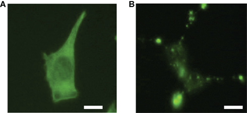
Figure 2. Representative photographs of the cells; negative control with 1/100 volume of DMSO (A); and treated with 2 μM final concentration CytB (B). Actin filaments of these cells were stained with Alexa488 conjugated phalloidin. The negative control cells have not changed their shape compared with non-treated cells. Cells treated with CytB showed aggregation of actin molecules while adherence to the bottom of the culture chamber was maintained. The scale bars represent 10 μm.

Under this condition, we confirmed the spatial distribution of actin aggregation and GFP in cells (Figure A1 in Appendix). GFP distribution was uniform in control cells (Figure A1A in Appendix, upper left panel and lower panel), and the distribution was not changed by CytB treatment (Figure A1B in Appendix, upper left panel and lower panel). On the other hand, actin filaments exist in the vicinity of cellular membrane in control cells (Figure A1A in Appendix, upper right panel and lower panel). After CytB treatment, actin filaments were broken up and produced aggregation but staying at the vicinity of cellular membrane (Figure A1B in Appendix, upper right panel and lower panel). These observations mean that GFP and actin do not interact neither do not move together in vivo environment.

Results from these experiments implied that CytB-treated cells did not much change their volume, also the aggregation of actin produced by this reagent did not trap transfected GFP; hence the total protein concentration did not differ from those in normal cells, but cytoskeletal structures were disrupted.

We analyzed the anomaly parameter of five CytB-treated cells (Table 2), obtaining α = 0.796 ± 0.056. The mean value we obtained from CytB-treated cells is closer to that expected under normal diffusion condition (α = 1). However by considering the range of the SD, the difference between control cells (negative control with DMSO) and CytB-treated cells was unclear. To confirm the possibility of that anomalous character of diffusion constant may depend more on the physiologically organized intracellular structures than on the intracellular protein concentration, we performed FCS analysis with the cells disrupted their cytoskeletons by the other reagent, in this case colchicine, an inhibitor of tubulin polymerization.

TABLE 2

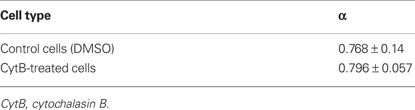
Table 2. Anomaly parameters of control cells and CytB-treated cells.

3.1.3 The effect of colchicine treatment

The effect of actin disruption was not clear, so we performed another experiment to confirm the effect of cytoskeletal disruption by using colchicine. Treatment with colchicine inhibits the polymerization of tubulin into microtubule. We performed 270 times FCS analysis with colchicine treated L-929 cells together with 48 times analysis of solvent-treated (EtOH) control cells. Because of the effect of the solvent (EtOH) of colchicine, the anomaly parameter of control cells (mean: 0.585 ± 0.28, mode: 0.68) was smaller than non-treated cells also than DMSO treated cells. However, the basic effect of microtubule disruption was similar with the effect of actin polymer disorders (Figure A2 in Appendix). The anomaly parameter of colchicine treated cells is approximately 0.02 closer to 1.0 than that of the control cells (mean: 0.602 ± 0.085, mode: 0.71). This is the same tendency with the case of actin disruption (anomaly parameter of CytB-treated cells was approximately 0.03 closer to 1.0 than that of control cells).

The wide range of SD of control cells made the effect of cytoskeletal disruption unclear; as the result we could not say there is a meaningful difference between the anomaly parameter values of control cells and of cytoskeleton disruptor-treated cells by statistical analysis. We may mention here that there is no clear contradiction to say keeping physiological cytoskeletal structure is effective to increase anomaly characteristics of in vivo environment.

3.2 Fractal Dimensions Analyzed Using TEM

Next we investigated the dimensionality of intracellular structures. We applied the box counting method to 165 TEM images of rat fibroblast 3Y1 cells, using the algorithm indicated in the Section 2 (Chhabra et al., 1989) to derive d_f.

We estimated two d_fs of two distinct segments in the cell images as explained in the Introduction. The Md_f was calculated for the white segments in the binarized TEM images (white segment in Figure 3A), while the Sd_f was calculated for the outline of the solid structures in the TEM images (Figure 3B). We tested whether these two d_fs are statistically different or the same (Table 3). Applying the MW-test, we infer that the probability of that these two d_fs are the same (P) is less than 0.01.

FIGURE 3

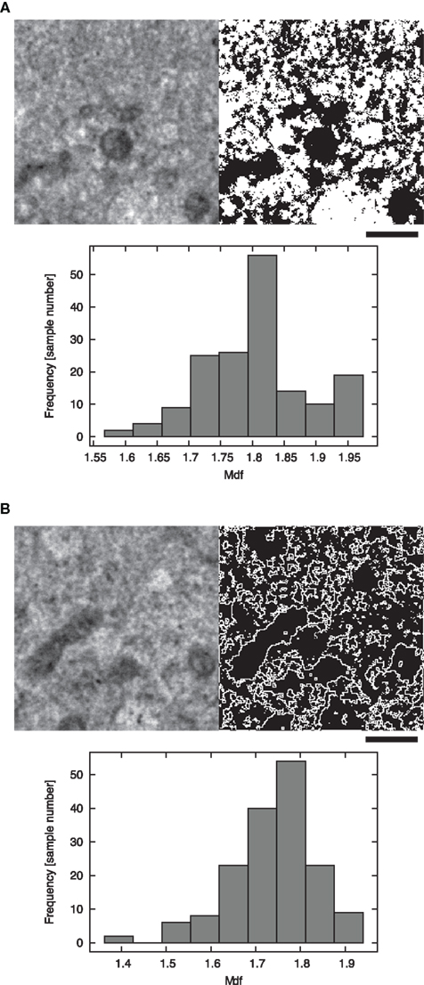
Figure 3. Fractal dimension calculation from the material TEM images of rat fibroblast 3Y1 cells. (A) Image data from which we obtained Md_f. The left and right panels display the original TEM and binarized images respectively. The histogram (bottom) displays the relationship between the value of the Md_f (lateral) and the frequency of occurrence (vertical). (B) The data from which we computed Sd_f. The left panel displays the original image. The image was once processed into a binary image (A); afterward, binary images were used to estimate d_f of the mobile area in cytoplasmic material. The histogram shows the relationship between the value of Sd_f (lateral) and frequency of occurrence (vertical). The scale bars represent 1 μm.

TABLE 3

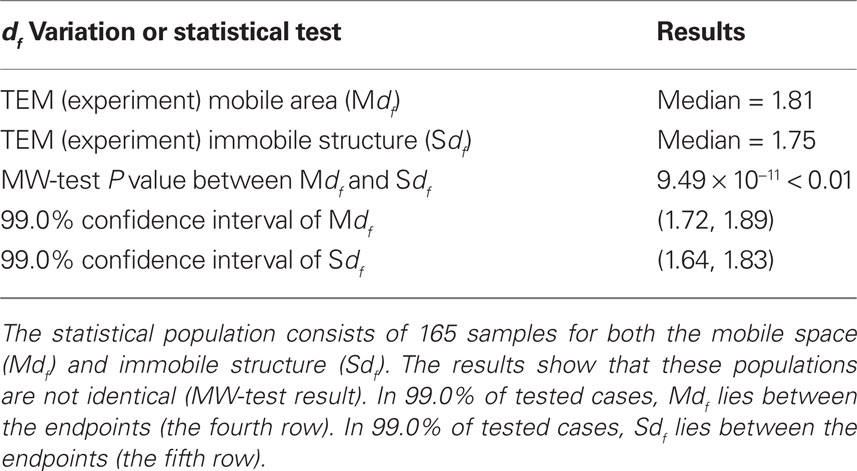
Table 3. Statistical analysis of two intracellular d_f.

We proceeded to examine which fractal models can explain the effect of the intracellular environment on free molecules, and therefore which models are candidates for understanding the organizing processes of the intracellular structure.

The median value of the Md_f was 1.81, the mean value and the SD of the Md_f = 1.81 ± 0.083. This result suggests that, in 99.0% of cases, Md_f lies between 1.72 and 1.89. This interval includes only the d_f value of IP model (d_f = 1.89, Table 1). The lower endpoint of the confidence interval is larger than all the other d_f values of percolation models, but close to the d_f value of DLA (1.71). On the other hand, the median value of the estimated Sd_f was 1.75, with mean value and its SD of the Sd_f = 1.74 ± 0.096. In 99.0% of cases, Sd_f will lie between 1.64 and 1.83. This interval includes only the d_f of DLA model (d_f = 1.71, Table 1). Even accounting for 99.0% of cases, the lower endpoint of the confidence interval is 1.64, significantly larger than the d_f of rlCCA model (=1.55). The higher endpoint was 1.83, which is smaller than the d_f predicted by the IP model (Tables 1 and 3).

3.3 The Effect of Two Noises

In order to examine whether those values of fractal dimension are robust against noises, we prepared four different data sets with adding two types of noises. One type of the noises is Gaussian noise. This type of noise is included when the microscope has a problem; for example the problem of magnetic lens, thermal noise originated from surrounding electronic circuit, and so on. This noise is estimated that the occurrence probability can be modeled with Gaussian distribution. We prepared two strength of the noise to our TEM image set, respectively. The other type of noises is impulse (salt and pepper) noise. Generally this type of noise is included during transferring the data, and appears with white and black dots with fixed probability. We also prepared two strength of the noise to our TEM image set, respectively. For TEM analysis, noise can be added during the sample preparation.

The results showed that Gaussian noise does not change the df values that much but dilutes the specific characteristics of each image (Table 4). On the other hand, impulse noise does not affect Md_f, but greatly changes the value of Sd_f. These results suggest that keeping good maintenance of microscope and checking the condition at each analysis are important, also to avoid the miss preparation of materials is needed to find clear characteristics of each structure in a cell. On the other hand, the basic values of intracellular d_fs were kept between the d_fs of DLA and IP models (1.71 and 1.89).

TABLE 4

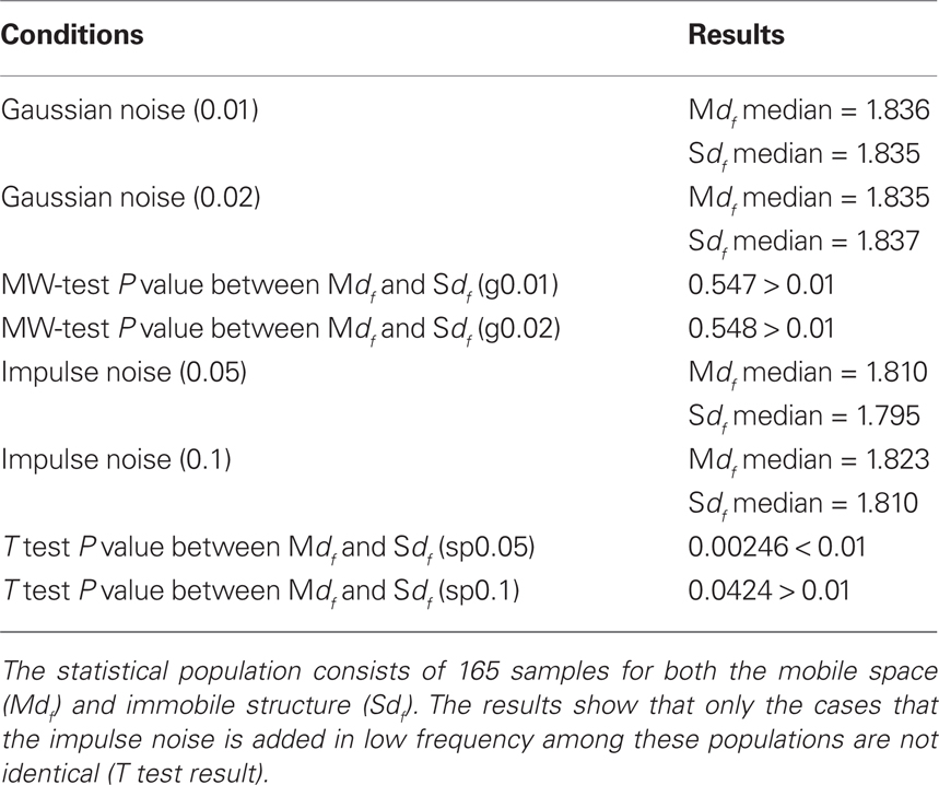
Table 4. Noise effect examination at d_f calculation by TEM images.

3.4 Estimation of the Spectral Dimension

Next we estimated d_s from the mean of α and Md_f values, which were obtained from Sections 2.2 and 2.3 by Eq. 10.

Not only the d_s value derived from Md_f but also the d_s value derived from Sd_f (1.34 ± 0.084) were close to the theoretically expected value (1.32; Alexander and Orbach, 1982), and the values estimated by numerical simulations (1.2–1.4; Meakin and Djordjevi, 1985). We used the d_s which was derived from Md_f instead of Sd_f for further analyses by following two reasons; first, our original assumption is that the area expressed by Md_f is the space for free molecular movement. This reason is important for the objective of analyzing d_s. The second is the robustness of this value against noises. Md_f was less affected by the noises, which means the result we obtain here by using this value will be easily reproduced in the other place and opportunity. Because of the above reasons, we used the d_s derived from Md_f in further analyses instead of the d_s derived from Sd_f. The median value of d_s derived with Md_f among 165 estimates is 1.39.

From the expression,

This result suggests that a reaction at the initial time occurs faster in vivo than for the time-independent reaction, which corresponds to reactions in a homogeneous well-diluted environment (Figure 4A).

FIGURE 4

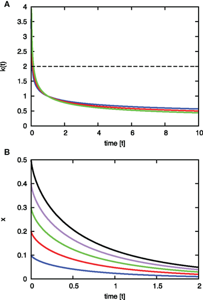
Figure 4. Estimated characteristics of the value d_s (A) The curve of k(t) = t^{−0301 ± 0. 056}. k(t) (y axis) is plotted as a function of t (x axis). Results are shown for minimum (blue), average (red), and the maximum (magenta) case of the exponent of t among the range. Characteristics of the k(t) lines show that any constant k > 0 is smaller than k(t) at first but later exceeds this time-dependent function. The dashed black line (k = 2) is an example case. k (=2) is smaller than any k(t) line at the beginning of the reaction, and afterward it overcomes k(t). This means that the reaction governed by this function starts rapidly in the inhomogeneous environment, but later slow down (relative to the classically assumed homogeneous environment). (B) Solution of the differential equation dx/dt = −k(t)x. The solution is The variation of the lines depends on the variation of a constant c₁ from 0.1 to 0.5, which appears in the right-hand term when we re-express the result as

We also obtained the solution of the differential equation

to estimate the fluctuation of the reactant of a time-dependent reaction described by Eq. 11.

The solution of the differential equation is

The fluctuation of x (the concentration of reactant) in Eq. 12 is shown graphically in Figure 4B.

Experimental results therefore suggest that physiological structural conditions induce quick response in the initial stages of a reaction, but later prevent the exhaustion of the reaction source.

3.5 Reaction Process Simulation in 3D Space with Hinder Molecules and Anomalous Diffusion Exponent Estimation

Next we tested whether the estimated reaction process, as inferred from our experiments, is consistent with the simulation results which reconstructed a reaction in an inhomogeneous, crowded environment. We performed Monte-Carlo simulation to investigate the reaction processes in a pseudo-inhomogeneous 3D space represented by adding NRO randomly to the reaction space.

Simulation results showed that k(t) behaves almost as a constant when NRO occupy less than 30% [Figure 5A, green = 0%, orange = 10%, pink = 20%, brown = 30%; line color = relative NRO volume(%)]. When the NRO occupancy of the simulation space is close to the percolation threshold, the behavior of k(t) is similar to the results obtained from experiments [Figures 4A and 5A, magenta = 40%, light blue = 50%, blue = 55%, red = 60%, light green = 65%; line color = relative NRO volume(%), and Figure A4 in Appendix].

FIGURE 5

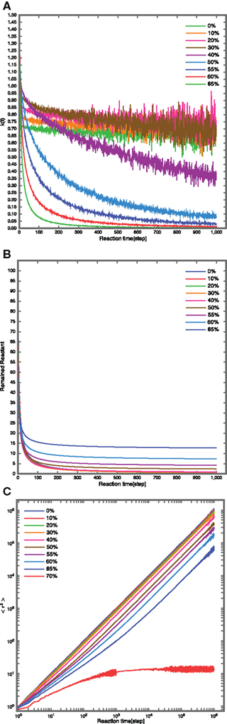
Figure 5. Simulation Results in 3D space with non-reactive obstacles (NRO).(A) Fluctuation of k(t) with time. When less than 30% of 3D space is occupied by the NRO, k(t) behaves similarly to a constant (green line = 0%, orange = 10%, magenta = 20%, brown = 30%). With NRO occupant close to the percolation threshold, behavior of k(t) becomes similar to experimentally observed behavior. (B) Time course fluctuation of reactant concentration. When the NRO occupancy is close to percolation threshold (blue = 65%, cyan = 60%), the fluctuation of the reactants shows a “quick response and slow exhaustion” pattern. This result compares well with that presented in Figure 4B. (C) The behavior of mean-square displacement (MSD). At 0% NRO occupancy, MSD behaves as a normal diffusion. Between occupancies of 10% (red) and 40% (magenta), MSD exhibits hindered diffusion behavior. At over 40% occupancy and up to the percolation threshold (60% = purple), the plot of MSD versus reaction time is concave, consistent with directed diffusion. Beyond the percolation threshold (70% = cyan), the curve becomes convex, indicating confined diffusion.

On the other hand, time course fluctuation of the reactant concentration showed that when NRO occupancy approaches the percolation threshold (blue = 65%, cyan = 60%), the reactant fluctuations exhibit “quick response and slow exhaustion” pattern (Figure 5B). This result compares favorably with the result indicated in Figure 4B.

Finally, we analyzed the behavior of MSD with respect to the relative amount of NRO in the simulation space (Figure 5C). At NRO 0%, MSD exhibits normal diffusion pattern. Between NRO occupancies of 10% (red) to 40% (magenta), MSD appears to exhibit hindered diffusion behavior. At NRO occupancies over 40% up to the percolation threshold (60% = purple), the plot of MSD versus reaction time develops a concavity, consistent with directed diffusion. When NRO occupancy is over the percolation threshold (70% = cyan), the curve becomes convex with lower value of normal diffusion case (the line of 0%), indicating confined diffusion.

Generally, the characteristics of a reaction process change at the percolation threshold (defined as the ratio between the lattice sites occupied by obstacles and free lattice sites; [68.8: 31.2 (%)] in 3D space). For concentrations of initial reactants up to the percolation threshold, reactions are accelerated at the beginning of the reaction, but the final concentrations of the products are lower as the ratio increases (Figure 5).

The estimated anomalous diffusion exponents that were dependent on the ratio are shown in Table 5. Values near the percolation threshold (60%) are close to the value calculated from FCS data (0.768 ± 0.14).

TABLE 5

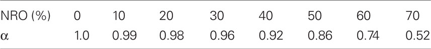
Table 5. Anomalous diffusion exponent values of each occupancy of non-reactive obstacles (NRO) in the reaction space.

These simulation results are compatible with our experimental results. Both experiments and computational simulation demonstrate that in vivo reactions undergo quick response and slow exhaustion reaction processes. Furthermore, simulation revealed that the difference between in vitro and in vivo imposed by the environmental conditions is strongly correlated with the percolation threshold.

4 Discussion

The intracellular environment is densely crowded and inhomogeneous as has been observed (Medalia et al., 2002). Diffusion of a molecule within a cell is restricted to the space between obstacles. To model diffusion-mediated processes, including modeling of kinetics, it is necessary to account for the effects of high concentrations of mobile reagents and immobile, non-reactant obstacles.

Diffusion occurring in such an environment is expected to differ from the normal diffusion of a pure random walker. In normal diffusion, the MSD is proportional to time, and the diffusion coefficient is constant. Anomalous diffusion is known to produce non-linear temporal behavior; the form of the time dependence is proportional to some power of time less than one (α). From this relationship, we infer a time-dependent diffusion coefficient for reactants in inhomogeneous, dense environments, of the form

which decreases to zero as t → ∞, where Γ is a constant. Mathematically anomalous diffusion is the result of deviations from the central limit theorem (Bouchaud and Georges, 1990); physiologically, it emerges from the presence of obstacles and traps.

We analyzed the anomaly parameter of GFP diffusion in cytoplasm (Figure 1). Our results indicated that the time-dependent form of the GFP diffusion is anomalous. Comparison with results from computational simulation (Table 5) yielded an estimated relative volume of NRO; it is approximately 60–70% (Figure 1B and Table 5) in the cytoplasm.

With regards to cellular physiology, this result is compatible with reliable reports of protein–water proportion in a cell, which comprises of 60% protein and 40% water (Fulton, 1982).

We investigated whether the total concentration of protein in a cell affects reaction kinetics in the intracellular environment, or whether organized cell structure plays a dominant role. We tested our ideas physiologically by subjecting CytB-treated cells and colchicine treated cells to FCS analyses (Figure 2, Table 2 and Figure A2 in Appendix), also by numerical simulation (Figure A3 in Appendix). Cytochalasin B disrupts the equilibrium condition between the actin polymer and the monomer. Colchicine inhibits tubulin polymerization into microtubule. The disruption of these cytoskeletal filaments while maintaining the total protein concentration changed the anomaly parameter, bringing it closer to the normal condition. This result suggests that not merely the concentration of intracellular proteins, but also their physiological organization profoundly affects diffusion of free molecules in a cell. And this conclusion is supported by our simulation results. When the same volume of NRO with randomly distributed NRO is shaped cube in the reaction space, reactants did not show anomaly characteristics.

There exists one interesting tendency among the condition of reaction space, which is represented by α values and their SD. In ideal in vitro space, α = 1 ± 0. In our results, the condition of cytoplasm of control cells is anomalous, at the same time widely varied the level of the anomaly which is represented by α. When we disordered cytoskeletal structures by chemical reagents, the condition of cytoplasm was still anomalous but the variety of anomaly was reduced. This seems natural if cytoskeletal disorganization changed intracellular environment from inhomogeneous space into homogeneous space. Further investigation is required to get clear conclusion from this point of view.

Fractals are self-similar, meaning that they exhibit similar fine-scale features at many magnifications. It was argued over 20 years ago that folded polymers, including chromatin, were fractals (Grosberg et al., 1988). Two recent reports have suggested that chromatin and the nucleoplasmic space surrounding it should be added to the fractal list (Bancaud et al., 2009; Lieberman-Aiden et al., 2009). In order to decide whether chromatin or its surrounding nucleoplasmic space is truly fractal, we need to visualize the structures directly.

We used TEM to directly obtain values of cytoplasmic d_f (Figure 3). The Sd_f is the fractal dimension of the surface of the intracellular structures (Figure 3B). Our Sd_f value is similar to those of DLA structures. This result suggests that intracellular structures may be organized in a diffusion-limited manner.

During the 1980s, numerical analyses were performed to estimate the d_s value of DLA. The estimated values are between d_s = 1.2–1.4 (Meakin and Djordjevi, 1985). Also theoretical analysis estimated d_s value as 1.32 (Alexander and Orbach, 1982). From our experimentally obtained results, we deduced a d_s of Sd_f (equaling the d_f of a DLA like intracellular structures), it is 1.34 ± 0.084. Even there remains the possibility to be argued about the noise and threshold effects, the derived d_s value is supportive to estimate our assumption is proper for this analysis. Our calculation procedure for d_s is modified to accommodate experiments with real cell materials. In the numerical analysis, d_w and d_f are both used. Here d_w is the dimension of a random walker on a fractal structure. On the other hand, since we can readily analyze α experimentally (e.g., by FCS): we chose to use α and d_f. Parameters derived from experimental techniques were compatible with those obtained from previous numerical simulations and theoretical works. We also confirmed the compatibility of our experimental results with our original numerical derivation of α. We therefore conclude that our procedure is appropriate for experimental estimates of d_s, and applicable further investigation of modeling reaction kinetics.

The Md_f is the fractal dimension of the space between intracellular structures, supposedly the space available to a diffusing molecule. The value of Md_f is similar to the d_f of an IP cluster. This result suggests that a molecule diffusing within intracellular space follows the rules of percolation.

The inference from our Md_f result does not contradict our further investigation of reaction form and the numerical simulation results. The both reaction form estimated from the d_s value and stochastic model, which included NRO in its reaction space, exhibited the same characteristics; that is quick response at the early stages of a reaction and slow exhaustion after a long times (Figures 4 and 5). The ratio of NRO in the reaction space in our simulation was close to the percolation threshold. All these results are consistent and support each other.

The results of our numerical simulation of MSD are of special interest. The curvature of the MSD versus reaction time plots depends on the relative volume of NRO in the reaction space (Figure 5C). When NRO is absent from the reaction space, the MSD of the reagent is linear in time. This case indicates the case of normal diffusion. While the spatial occupancy of NRO is below 40%, the curve appeared linear but the slope become smaller, indicating hindered diffusion. As the occupancy of NRO approaches the percolation threshold, the curve develops a concave form. Among the diffusion models, directed diffusion (MSD = 2dD₀t + v²t², where d is the Euclidean dimension, D₀ is the diffusion coefficient of normal diffusion, and v is the velocity of a flow in the reaction space) appears to best describe this phenomenon. When NRO occupancy exceeds the percolation threshold, the curve developed signs anomalous or confined diffusion.

Therefore, such an environment may boost the diffusion velocity of a molecule if our result is correct in environments supporting NRO occupancies slightly less than the percolation threshold. Since diffusion velocity affects the reaction rate, such an environment may accelerate or enhance biochemical reactions. This phenomenon may explain the quick response at the first stage of a reaction in such a crowded space.

In conclusion, the d_f value of static structures (Sd_f) in a cell is close to the d_f of diffusion-limited self-organizing aggregation. Furthermore, estimating the behavior of reactants between the aggregations is found to resemble the behaviors of molecules in the vicinity of critical percolation, as evidenced by d_f of the reactant space being close to d_fs of IP.

Similar results have been obtained by comparing numerical simulation and in vitro self-organization of fibronectin, a component of the extracellular matrix (Berry, 2008). This in vitro observation suggests that physiological molecules self-organize into a fractal structure. Our results suggest that actual intracellular structures organize similarly. Additionally, such an environment renders the reaction form time-dependent, favoring a quick response – slow exhaustion process over a slow response – quick exhaustion by constant production process, which continues until all the resources have been exhausted. The cause of both the initial quick response and remaining reaction sources could be the percolation cluster-like environment itself.

This property of in vivo reaction processes potentially affects the characteristics of entire biochemical networks.

We are planning to analyze a system level dynamics of biochemical network which includes such in vivo reaction processes and compare the dynamics with equivalent in vitro network. This investigation might suggest the characteristics of a living system.

Our results are applicable to aid the construction of precise in vivo oriented models.

Conflict of Interest Statement

The authors declare that the research was conducted in the absence of any commercial or financial relationships that could be construed as a potential conflict of interest.

Acknowledgments

We are deeply grateful to Professor Kazunori Nakajima (Department of Anatomy, School of Medicine, Keio University) who kindly arranged our first meeting among Department of Pathology and Department of Biosciences and Informatics in our university. We are grateful to Dr. Kayoko Suenaga (Carl Zeiss MicroImaging Co., Ltd.) for her kind helps and big effort to perform FCS analysis with colchicine treated L-929. We are also grateful to the following people and companies who edited our manuscript; MB Brad Fast (Fastek Ltd.); Dr. Leonie Pipe (Edanz Group Ltd.). We finally would like to express our deep gratefulness to Dr. Tetsuya J. Kobayashi (Institute of Industrial Science, the University of Tokyo) for his ceaseless helps and many of kind advises.

Funding

This work is supported by SUNBOR grant (provided by SUNTORY Institute for Bioorganic Research, Japan), and by a Viennese Science and Technology Funds WWTF, project grant MA07-30.

References

Alexander, S., and Orbach, R. (1982). Density of states on fractals: fractions. J. Phys. (Paris) Lett. 43, L625–L631.

Aon, M. A., O’Rourke, B., and Cortassa, S. (2004). The fractal architecture of cytoplasmic organization: scaling, kinetics and emergence in metabolic networks. Mol. Cell. Biochem. 256/257, 169–184.

CrossRef Full Text

Atkins, P., and de Paula, J. (2006). Elements of Physical Chemistry, 4th Edn, Oxford: Oxford University Press.

Bancaud, A., Huet, S., Daigle, N., Mozziconacci, J., Beaudouin, J., and Ellenberg, J. (2009). Molecular crowding affects diffusion and binding of nuclear proteins in heterochromatin and reveals the fractal organization of chromatin. EMBO J. 28, 3785–3798.

Pubmed Abstract | Pubmed Full Text | CrossRef Full Text

Berry, H. (2002). Monte Carlo simulations of enzyme reactions in two dimensions: fractal kinetics and spatial segregation. Biophys. J. 83, 1891–1901.

Pubmed Abstract | Pubmed Full Text | CrossRef Full Text

Berry, H. (2008). Modeling Complex Biological Systems: Examples in Computational Cell Biology, Computational Neurology and application to Computer Science. ThÉse d’habilitation á diriger des recherches. Paris: Centre de Recherche Saclay-âle-de-France et LRI, UMR 8623 CNRS et UniversitÉ Paris-Sud 11.

Bouchaud, J. P., and Georges, A. (1990). Anomalous diffusion in disordered media: statistical mechanisms, models and physical applications. Phys. Rep. 195, 127–293.

CrossRef Full Text

Broadbent, S. R., and Hammersley, J. M. (1957). Percolation processes. Math. Proc. Camb. Philos. Soc. 53, 629–641.

CrossRef Full Text

Chhabra, A. B., Meneveau, C., Jensen, R. V., and Sreenivasan, K. R. (1989). Direct determination of the f(α) singularity spectrum and its application to fully developed turbulence. Phys. Rev. A 40, 5284–5294.

Pubmed Abstract | Pubmed Full Text | CrossRef Full Text

Dobrescu, G., Crisan, M., Zaharescu, M., and Ionescu, N. I. (2004). Fractal dimension determination of sol–gel powders using transmission electron microscopy images. Mater. Chem. Phys. 87, 184–189.

CrossRef Full Text

Einstein, A. (1905). Über die von der molekularkinetischen Theorie der Wärme geforderte Bewegung von in ruhenden FÜssigkeiten suspendierten Teilchen. Ann. Phys. 17, 549–560.

CrossRef Full Text

Fulton, A. B. (1982). How crowded is the cytoplasm? Cell 30, 345–347.

Pubmed Abstract | Pubmed Full Text | CrossRef Full Text

Gefen, Y., Aharony, A., and Alexander, S. (1983). Anomalous diffusion on percolating clusters. Phys. Rev. Lett. 50, 77–80.

CrossRef Full Text

Grosberg, A. Y., Nechaev, S. K., and Shakjnovich, E. I. (1988). The role of topological constraints in the kinetics of collapse of macromolecules. J. Phys. France 49, 2095–2100.

CrossRef Full Text

Hiroi, N., Lu, J., Iba, K., Tabira, A., Yamashita, S., Okada, Y., Köhler, G., and Funahashi, A. (2011). A Study into the Crowdedness of Intracellular Environment: Estimation of Fractal Dimensionality and Anomalous Diffusion. Available at: http://www.wcsb2011.ethz.ch/ [WCSB2011].

Jackson, M. B. (2006). Molecular and Cellular Biophysics. Cambridge: Cambridge University Press.

Kohler, R. H., Schwille, P., Webb, W. W., and Hanson, M. R. (2000). Focal volume optics and experimental artifacts in confocal fluorescence correlation spectroscopy. J. Cell Sci. 113, 3921–3930.

Pubmed Abstract | Pubmed Full Text

Kopelman, R. (1988). Fractal Reaction Kinetics. Science 241, 1620–1626.

Pubmed Abstract | Pubmed Full Text | CrossRef Full Text

Kopelman, R. (1991). Exciton Microscopy and Reaction Kinetics in Restricted Spaces. Phys. Chem. Mech. Mol. Radiat. Biol. 1, 457–502.

Lieberman-Aiden, E., van Berkum, N. L., Williams, L., Imakaev, M., Ragoczy, T., Telling, A., Amit, I., Lajoie, B. R., Sabo, P. J., Dorschner, M. O., Sandstrom, R., Bernstein, B., Bender, M. A., Groudine, M., Gnirke, A., Stamatoyannopoulos, J., Mirny, L. A., Lander, E. S., and Dekker, J. (2009). Comprehensive mapping of long-range interactions reveals folding principles of the human genome. J. Phys. France 49, 2095–2100.

Malchus, N., and Weiss, M. (2010). Elucidating anomalous protein diffusion in living cells with fluorescence correlation spectroscopy – facts and pitfalls. J. Fluoresc. 20, 19–26.

Pubmed Abstract | Pubmed Full Text | CrossRef Full Text

Masuda, A., Ushida, K., and Okamoto, T. (2005). New fluorescence correlation spectroscopy enabling direct observation of spatiotemporal dependence of diffusion constants as evidence of anomalous transport in extracellular matrices. Biophys. J. 88, 3584–3591.

Pubmed Abstract | Pubmed Full Text | CrossRef Full Text

Meakin, P., and Djordjevi, Z. B. (1985). Cluster–cluster aggregation in two-monomer systems. J. Phys. A Math. Gen. 19, 2137–2135.

CrossRef Full Text

Meakin, P., and Stanley, H. E. (1983). Spectral dimension for the diffusion-limited aggregation model of colloid growth. Phys. Rev. Lett. 51, 1457–1460.

CrossRef Full Text

Medalia, O., Weber, I., Frangakus, A. S., Nicastro, D., Gerisch, G., and Baumeister, W. (2002). Macromolecular architecture in eukaryotic cells visualized by cryoelectron tomography. Science 298, 1209–1213.

Pubmed Abstract | Pubmed Full Text | CrossRef Full Text

Parus, S. J., and Kopelman, R. (1989). Self-ordering in diffusion-controlled reactions: exciton fusion experiments and simulations on naphthalene powder, percolation clusters, and impregnated porous silica. Phys. Rev. B Condens. Matter 39, 889–892.

Pubmed Abstract | Pubmed Full Text | CrossRef Full Text

R Development Core Team. (2011). R: A Language and Environment for Statistical Computing. R Foundation for Statistical Computing. Available at: http://www.R-project.org/

Rigler, R., Mets, Ü., Widengren, J., and Kask, P. (1993). Fluorescence correlation spectroscopy with high count rate and low background: analysis of translational diffusion. Eur. Biophys. J. 22, 169–175.

CrossRef Full Text

Schnell, S., and Turner, T. E. (2004). Reaction kinetics in intracellular environments with macromolecular crowding: simulations and rate laws. Prog. Biophys. Mol. Biol. 85, 235–260.

Pubmed Abstract | Pubmed Full Text | CrossRef Full Text

Snedecor, G. W., and Cochran, W. G. (1989). Statistical Methods, 8th Edn, Ames, IA: Iowa State University Press.

Stauffer, D., and Aharony, A. (1994). Introduction to Percolation Theory, 2nd Edn. London: Taylor & Francis.

Tolman, S., and Meakin, P. (1989). Off-lattice and hypercubic-lattice models for diffusion-limited aggregation in dimensionalities 2–8. Phys. Rev. A 40, 428–437.

Pubmed Abstract | Pubmed Full Text | CrossRef Full Text

Weiss, M., Elsner, M., Kartberg, F., and Nilsson, T. (2004). Anomalous subdiffusion is a measure for cytoplasmic crowding living cells. Biophys. J. 87, 3518–3524.

Pubmed Abstract | Pubmed Full Text | CrossRef Full Text

Wilkinson, D., and Willemsen, J. F. (1983). Invasion percolation: a new form of percolation theory. J. Phys. A Math. Gen. 16, 3365–3376.

CrossRef Full Text

Appendix

The Effect of Threshold to Produce Binary Images

We tested the effect of threshold to calculate d_f. The reason we binarized the TEM images as the black and white area keep equal size is that the estimated volume from the mass (approximately 60% of a cell; Fulton, 1982) and general protein density (1.14, 1.30 g/ml) is approximately 50% (49.2%). Because this is approximate value based on the assumption, which the obstacles in a cell are made of protein, there remains the possibility that the approximation is too rough or the assumption is not proper. To estimate if the methodology we chose was precise or not, we changed the threshold value to 0.4 and 0.6 (the size ratio of black and white area will be 2:3 or 3:2, respectively) instead of 0.5 (which equals the size ratio of black and white area is 1:1), and investigated the effect of these changes. Obviously these alteration affect the area size for molecular movement where we assumed (the white area of binarized image). It is projected Md_f values will be changed from original.

The results showed that changing threshold brings a change to the values of d_fs (Table A1). All the estimated d_f become 1.6 to 1.7. These values are closer to the d_f value of reaction-limited Cluster–Cluster Aggregation (rlCCA) model (d_f = 1.55) than the results with threshold 0.5.

TABLE A1

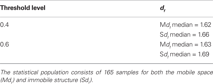
Table A1. Statistical analysis of two intracellular cellular d_f.

In rlCCA model, unit molecule behaves as Brownian particle; the probability they bind each other is infinitely close to zero. When aggregation is produced, the aggregation will be the new Brownian particle, the cluster-based units.

As we estimated, the change of Mdf is larger than the change of Sdf in this case. The both Sdf derived with the alternative threshold values (0.4 and 0.6) are still involved into the 99.0% confidence interval of Sdf derived with the original threshold (0.5).

There could be exist the cases, which a part of intracellular components are constructed with cluster-based units of molecules and the results from alternative thresholds fit better than the original to describe intracellular environment. Even such cases, it can be imagined from these results that the surfaces of the structures are rough as same as a structure constructed with single-molecular units. It will appear as the robustness of Sdf values against changing the thresold.

Our assumption in the article focused on the behaviors of single-molecular particle. The situation that a part of structural molecules is processed with small clusters is a probable hypothesis, but current knowledge which we used to decide the original threshold value seems inadaptable to choose the alternative thresholds. To adapt the different threshold and the models based on the results for accounting clustering units of polymers in a cell, we may need to find the other appropriate reason to change the threshold in the future.

FIGURE A1

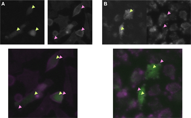
Figure A1. Cytohistochemistry of GFP and actin. Actin proteins observed that they localize at the vicinity of plasma membrane before the treatment [(A), upper left panel], and after the CytB treatment, actin proteins aggregated but did not move off from the vicinity of plasmamembrane [(B), upper left panel]. On the other hand, GFP spreaded homogeneously in a cell both the case of before and after CytB treatment [(A) and (B), upper right panels]. This means that these two proteins do not bind each other in a cell and not to be combined together by CytB treatment, neither do not move together [(A) and (B), lower panels].

FIGURE A2

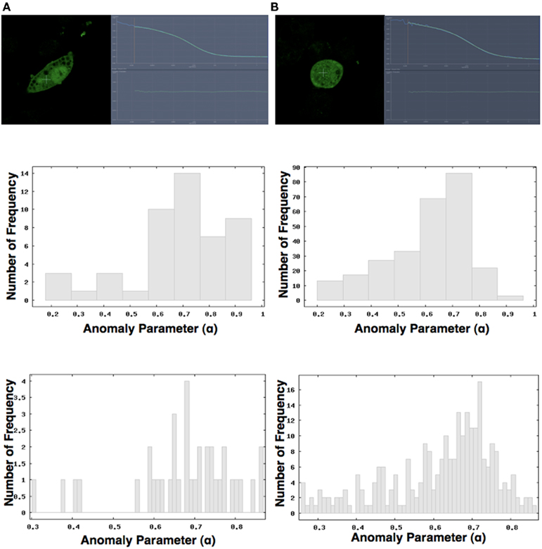
Figure A2. Fluorescence correlation spectroscopy analysis with colchicine treated cells (A). FCS analysis with control cells (EtOH treated). The top left panel is the image of a control cell, and the right panel is the example data of auto-correlation curve of FCS analysis. The histogram indicated in the middle panel shows the distribution of the value of anomalous parameter of control cells in eight ranges between 0.2 and 1. The bottom histogram indicates the distribution of the value of anomalous parameter of control cells in 55 ranges between 0.3 and 1 to show the mode value among the data clearly. (B) FCS analysis with colchicine treated cells. The top left panel is the image of a colchicine treated cell, and the right panel is the example data of auto-correlation curve of FCS analysis. The histogram indicated in the middle panel shows the distribution of the value of anomalous parameter of colchicine treated cells in eight ranges between 0.2 and 1.The bottom histogram indicates the distribution of the values of anomalous parameter of colchicine treated cells in 55 ranges between 0.3 and 1 to show the mode value among the data clearly.

FIGURE A3

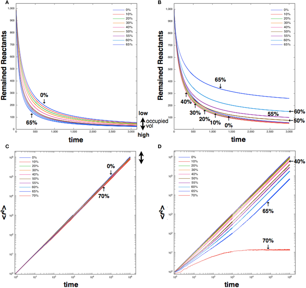
Figure A3. Simulation results in 3D space with different shape of NRO. We simulated if the shape of NRO clusters in the simulation space affect the reaction processes. The test was performed with cubic NRO (A, C) or random NRO (B, D). The upper panels (A, B) show the time course fluctuations of remained reactants. And the lower panels (C, D) show the time course fluctuations of MSD.

FIGURE A4

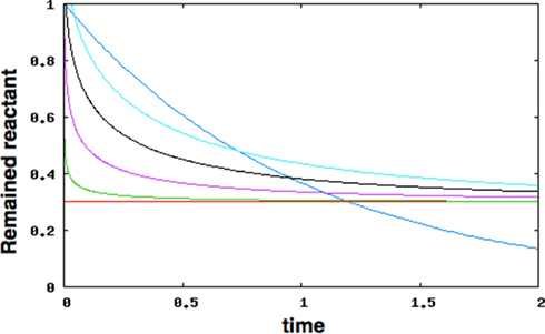
Figure A4. The fluctuation of remained reactant. The blue line is the case of homogeneous environment (k = −1, constant in d [reactant]/dt). The other lines are the case of df = 1.0, 1.2, 1.4, 1.6, 1.8, respectively (cyan, black, purple, green and red). This graph shows that when df takes a value between 1 ≤ df < 2, the reaction proceeds quick-response and slow exhaustion manner.