Genotype-phenotype map characteristics of an in silico heart cell

Understanding the causal chain from genotypic to phenotypic variation is a tremendous challenge with huge implications for personalized medicine. Here we argue that linking computational physiology to genetic concepts, methodology, and data provides a new framework for this endeavor. We exemplify this causally cohesive genotype–phenotype (cGP) modeling approach using a detailed mathematical model of a heart cell. In silico genetic variation is mapped to parametric variation, which propagates through the physiological model to generate multivariate phenotypes for the action potential and calcium transient under regular pacing, and ion currents under voltage clamping. The resulting genotype-to-phenotype map is characterized using standard quantitative genetic methods and novel applications of high-dimensional data analysis. These analyses reveal many well-known genetic phenomena like intralocus dominance, interlocus epistasis, and varying degrees of phenotypic correlation. In particular, we observe penetrance features such as the masking/release of genetic variation, so that without any change in the regulatory anatomy of the model, traits may appear monogenic, oligogenic, or polygenic depending on which genotypic variation is actually present in the data. The results suggest that a cGP modeling approach may pave the way for a computational physiological genomics capable of generating biological insight about the genotype–phenotype relation in ways that statistical-genetic approaches cannot.

Introduction

A comprehensive understanding of how genetic variation causes phenotypic variation of a complex trait is a long-term disciplinary goal of genetics (Bateson, 1906). The idea of linking system dynamics and genetics dates back to Burns (1970) and has proved fruitful in relatively simple cases (Omholt et al., 2000; Gilchrist and Nijhout, 2001; Peccoud et al., 2004; Welch et al., 2005; Gjuvsland et al., 2007a,b,c, 2010; Rajasingh et al., 2008; Martens et al., 2009). The basic premise is that in a well-validated model that is capable of accounting for the phenotypic variation in a population, the causative genetic variation will manifest in the model parameters. In this context, the term “phenotype” refers to any relevant measure of model behavior, whereas the term “parameter” denotes a quantity that is constant over the time-scale of the particular model being studied. However, model parameters are themselves phenotypes (Rajasingh et al., 2008), whose genetic basis may be mono-, oligo-, or polygenic, and whose physiological basis can be mechanistically modeled at ever deeper levels of detail. The term causally cohesive genotype–phenotype (cGP) modeling (Rajasingh et al., 2008) thus denotes an approach where low-level parameters have an articulated relationship to the individual’s genotype, and higher-level phenotypes emerge from the mathematical model describing the causal dynamic relationships between these lower-level processes. It aims to bridge the gap between standard population genetic models where the connection between genotypes and phenotypes is described in the form of “genotypic values,” i.e., the expected phenotypic value for a given genotype (Falconer and Mackay, 1996; Lynch and Walsh, 1998), and mechanistic physiological models without an explicit genetic basis. This forces a causally coherent depiction of the genotype-to-phenotype (GP) map.

Computational physiology is the natural habitat for this endeavor. Computational modeling of multiscale physiology is intimately tied to experimental studies and has offered unique and generic insights into medically important mechanisms (Noble, 2002b). Mechanistic models facilitate confrontation with empirical data, incorporating conservation of charge, mass and momentum, and other physical laws that serve to constrain the mapping from low-level parameters to higher-level phenotypes (Hunter and Borg, 2003). Dealing with genetic and other individual differences is a key next step (Hunter et al., 2010), which will require the incorporation of genotypic data and the application of multivariate numerical and statistical methods in computational physiology. The discipline thus defined may be called computational physiological genomics.

The mammalian heart is arguably the best available cGP model system, being studied in detail at levels from protein subunits through ion channels and calcium handling, cellular action potential (time-course of transmembrane voltage, V) and calcium transient (time-course of cytosolic Ca²⁺ concentration, Cai), tissue electrophysiology, mechanics, and fluid dynamics (Noble, 2002a). Much of this research has been medically motivated, as anomalies in these processes can give rise to disease in a complex interplay between genetic, age-related, and lifestyle factors. However, analyzing whole-organ models is computationally and conceptually challenging, and many submodels are of quite intimidating complexity in themselves.

Here, as a pilot for a whole-organ cGP study, we explore, characterize, and analyze a detailed model of a mouse heart cell (Li et al., 2010), built to account for the action potential (electrical signal) and calcium transient (linked to muscle contraction) of the cardiomyocyte in terms of its constituent ion currents and gating channels. Cardiac ion channels are prime candidates for realistic gene-to-parameter mapping, being quite low-level parameters whose genetic variation has been well studied (Roberts and Brugada, 2003; Roepke and Abbott, 2006; Sanguinetti and Tristani-Firouzi, 2006). Under the assumption that genetic variation manifests in low-level parameters, simulations of the model generate in silico high-dimensional phenotypes, ranging from individual ion currents to the action potential and calcium transient.

By use of the single heart cell cGP model we show (1) how the statistical-genetic architecture of traits may arise, (2) how multivariate analysis methods can be used to extract information about high-dimensional GP maps created by cGP models, (3) how the cGP framework can be used to identify genetic variation underlying disease phenotypes, and (4) how the cGP framework can be used to systematically disclose how the genetic background may affect penetrance, i.e., the proportion of affected individuals among those carrying a predisposing allele. The paper thus addresses several key disciplinary aspects of physiological genomics, and it exemplifies many of the methodological challenges pertaining to whole-organ models, while being computationally inexpensive enough to allow a more exhaustive exploration.

Methods

Heart Cell Model

The LNCS cell model (Li et al., 2010) extends that of Bondarenko et al. (2004) with more realistic calcium handling, detailed re-parameterization to consistent experimental data, and consistency checking by conservation of charge (cf. Hund et al., 2001). State variables include concentrations of sodium, potassium, and calcium in the cytosol, calcium concentration in the sarcoplasmic reticulum, and the state distribution of ion channels, whose transition rates between open, closed, and inactivated conformations may depend on transmembrane voltage. A simplified overview is given in Figure 1. The model is available as Supplementary Material in CellML and PDF formats. (For details, see Bondarenko et al., 2004; Li et al., 2010) Whereas many cell models are built from heterogeneous data sets that span species and temperature (Niederer et al., 2008), essential parts of the LNCS model have been directly fitted to a consistent experimental data set for the C57BL/6 “black 6” mouse, a popular strain for genetic manipulation in studying cardiac electrophysiology and the regulation of intracellular calcium transport. Formulated as a system of 35 coupled ordinary differential equations with 175 parameters (see Unhardcoding of Parameters below), this model provides a comprehensive representation of membrane-bound channels and transporter functions as well as fluxes between the cytosol and intracellular organelles. Below, the term “baseline” refers to the point estimate for the parameter values of the LNCS model, and phenotypes arising from simulations with the baseline parameter scenario.

FIGURE 1

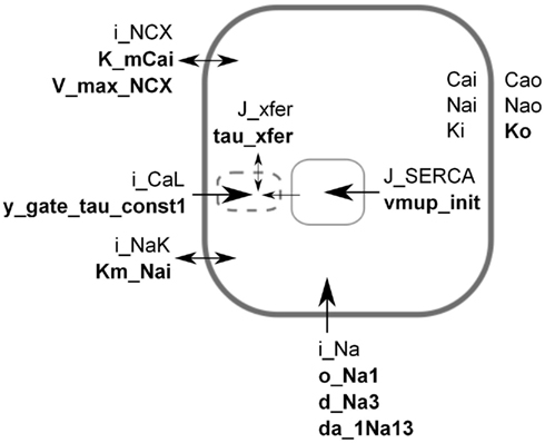
Figure 1. Simplified schematic of the LNCS mouse heart cell model. For the sake of illustration, each parameter in the model was assumed to have a monogenic basis, with parameter values for genotypes aa, Aa, AA having parameter values of 50, 100, and 150% of baseline. Based on an initial sensitivity analysis, the parameters shown (bold) were selected for a full factorial simulation experiment representing 3¹⁰ genotypes and their resulting phenotypes. The transmembrane potential is created by the difference in ion concentrations inside and outside the cell. Extracellular [Ca²⁺], [Na⁺], and [K⁺] are assumed constant, whereas the intracellular concentrations are state variables. Calcium is initially sequestered (J_SERCA) into the sarcoplasmic reticulum (SR, solid box) inside the cell. In response to an electric stimulus, the fast sodium current (i_Na) sets off an action potential that in turn triggers the release of calcium (J_xfer) via “dyadic space” microdomains (dashed box) where an early L-type calcium current (i_CaL) induces release of calcium from the SR. Parameters were selected to span a range of components and roles, see Table 1. Some components are strongly simplified in the figure, see Bondarenko et al. (2004), Li et al. (2010) for full description.

TABLE 1

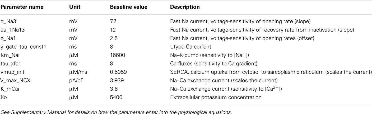
Table 1. Heart cell model parameters, assumed to reflect individual genes, that were varied (50, 100, 150) to simulate genetic variation.

Virtual Experiments and Phenotypes

We studied phenotypes defined by four experimental protocols described in Bondarenko et al. (2004). Voltage-clamp protocols induce series of stepwise changes in transmembrane voltage (items 3 and 4 below) that are designed to characterize the voltage-dependent conformation switching behavior and “memory” of ion channels (Molleman, 2002), offering a common basis for comparing the ion-channel behavior of different cell types, models, or parameter scenarios. The protocols were:

1. No stimulus, yielding the quiescent cell state as a phenotype.

2. Regular pacing from quiescence to steady-state dynamics or alternans (action potentials of alternating amplitude), implemented as an external stimulus current of K⁺ ions. Raw phenotypes were the multivariate time-series of state variables during a steady-state action potential (or series of action potentials in the case of alternans), as well as important terms in the rates of change, such as ion currents. The main cell-level phenotypes are the action potential (electrical signal) and calcium transient (linked to muscle contraction), i.e., the time-courses of the transmembrane potential and cytosolic calcium concentration, respectively. Aggregate measures for these phenotypes include action potential duration to 90% repolarization (APD90), similar measures for 25, 50, and 75% repolarization, and action potential amplitude and time to peak (Figure 2). APD decay rate, λ, was computed from the exponential approximation V(t) = V(0) exp(−λt) based on voltage and time from 50 to 90% repolarization. Analogous measures were used for the calcium transient.

A stimulus current of −15 V/s was applied for 3 ms at the start of each stimulus interval. This was repeated until convergence or a maximum of 10 min simulated model time. Convergence was checked by comparing successive intervals with respect to initial values of each state variable, as well as the integral of the state variable’s trajectory over that interval. A running history of 10 intervals was kept, and after each interval we checked for a match (within a relative tolerance of 1% for all state variables) against the previous ones. This was done for stimulus intervals of 100, 200, and 300 ms.

3. Double-pulse voltage-clamp protocol to estimate the rate and voltage-dependence of ion-channel inactivation. The simulated cell is initially kept at a low holding potential V_hold, followed by an abrupt increase to some voltage V₁ for duration t₁ (pulse P1), then set to some voltage V₂ (pulse P2). The main experimental parameters are the duration and voltage of pulse 1. Raw phenotypes are the same as for regular pacing, with emphasis on the total current (e.g., i_Na for the fast sodium current) and the proportion of ion channels in each conformation. Aggregate phenotypes include peak P1 current and the “rate of inactivation” τ, describing the roughly exponential decline in current during the first pulse (P1) as:

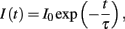
and fitted to the interval from 95 to 5% of the peak current.

4. Variable-gap voltage-clamp protocol to estimate the rate and voltage-dependence of recovery from inactivation. From the holding potential, an initial depolarizing pulse P1 will inactivate a high proportion of the ion channels, and is followed by a repolarizing interpulse interval of variable duration (the main experimental parameter), then another pulse P2. Current magnitude during P2 measures recovery from inactivation as a function of interpulse duration. The results were summarized by I_peak,max and t_half in the equation

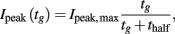
where t_g is the gap duration and I_peak is the peak P2 current.

FIGURE 2

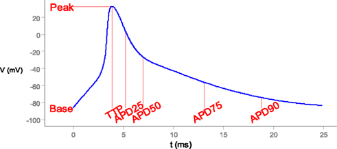
Figure 2. Scalar measures of state-variable trajectories, exemplified by the action potential. TTP, time to peak. APD25, etc.: action potential duration to 25%, etc., return to initial (“base”) value.

Disease Phenotype

Cell dynamics was categorized as “failed” based on the calcium transient if the peak was below 50% of baseline (illustrating failure to contract), if the base was more than 200% of baseline (failure to relax), if amplitude was less than 50% of baseline (at 200 ms pacing), or if dynamics failed to converge within 10 min of simulated time. Details of alternans were not pursued in this paper.

Unhardcoding of Parameters

Many, if not most, published cell models include constants that are arguably better viewed as parameters for the purpose of cGP studies, such as the voltage-sensitivity of ion-channel behavior. For example, the sodium channel of the Bondarenko model contains just one parameter but 28 hardcoded constants (Bondarenko et al., 2004, Eq. A51–A64). We used the Python package lxml 2.3¹ to scan a CellML (Lloyd et al., 2004) representation of the LNCS model for constants, except for physical constants (such as the Faraday constant) and ion charges (e.g., 2 for Ca²⁺). This brought the number of parameters up from 73 to 175, not counting physical constants or parameters relating to pacing protocols.

Local Sensitivity Analysis

For a local overview of the genotype-to-phenotype map, we estimated the first derivatives of scalar phenotype measurements Φ_k with respect to model parameters p_i, using central differences with a 10% step size. For parameters and phenotypes that have a non-arbitrary zero point, it is meaningful to scale the first derivatives into elasticities, i.e., dimensionless ratios of relative changes. This is equivalent to log-transforming the quantities before taking derivatives.

Thus, a q% change in p_i leads to a q × e_ik% change in Φ_k, assuming q is small. Based on this overview, we selected a few model genes for simulating all possible genotypes, using a full factorial design for their associated parameters.

Computer Implementation

Python code was auto-generated using the CellML code generation service at www.cellml.org. The equations were integrated using the CVODE solver (Cohen and Hindmarsh, 1996), with a Python wrapper for flexible scripting of virtual experiments. Phenotypes were computed with Python and Numpy (Oliphant, 2006). Statistical analyses were done in R 2.10.1 (R Development Core Team, 2011), using the packages “ggplot2” 0.8.3 (Wickham, 2009) for aggregation and plotting, and “pls” 2.1-0 (Mevik and Wehrens, 2007) for partial least squares (PLS) regression.

Results and Discussion

Design Patterns for CGP Studies

The workflow in Figure 3 exemplifies the design pattern (Wikipedia, 2010) we developed to facilitate the interchange and reuse of its components: the generation of genotypes (e.g., exhaustive enumeration or reduced designs), the mapping of genes to parameters (based on genome databases, e.g., Hancock et al., 2009), physiological models (Le Novere et al., 2006; Lloyd et al., 2008) that map parameters to phenotypes, virtual experiments to generate phenotypes that are defined by the model system’s response to some stimulus or perturbation (e.g., voltage clamping, Molleman, 2002), and aggregation from model dynamics to clinically relevant phenotypes (e.g., action potential duration). This pipeline design allows the gluing together of appropriate tools for each task. For instance, experimental designs and statistical analyses were done in R (R Development Core Team, 2011), whereas virtual experiments were flexibly described in Python² (see also Langtangen, 2009). The general approach should apply equally well to eventual whole-organ cGP studies.

FIGURE 3

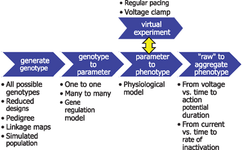
Figure 3. Simulation pipeline for causally cohesive genotype–phenotype studies. Blue arrows denote functions that generate genotypes or transform them through successive mappings, genotype to parameter to “raw” phenotypes to aggregated phenotypes. The surrounding text exemplifies different alternatives for each piece of the pipeline, e.g., a simple mapping of variation at one locus to variation in one parameter, or a more mechanistic gene regulatory model. “Virtual experiments” interact with physiological models to generate phenotypes defined by the system’s response to external stimuli.

Genotype–Phenotype Elasticities

Figure 4 gives a broad overview of the effects of genetic parameter variation on higher-level phenotypes (defined in Figure 2), formulated as elasticities (ratios of relative changes) where applicable. Working with relative changes provides biologically interpretable measures while being dimensionless. For example, the elasticity to Ko (a concentration) of action potential duration to 90% repolarization (a time) was estimated at 0.45 under pacing at 100-ms intervals. Although this number is dimensionless, we find it helpful to think in terms of “percent per percent.” Thus, a 10% increase in Ko would result in about a 4.5% increase in APD90. For quantities without an absolute zero, however, relative changes are not meaningful, and sensitivity measures must be expressed using absolute units for either or both of the phenotype and genotypic parameter. For example, the sensitivity of peak voltage to o_Na2 at 100 ms pacing was −1.45 mV per mV; the absolute change in peak voltage per relative change in d_Na3 was −98 mV, or −0.98 mV peak voltage per percent d_Na3; and the relative change in inactivation time τ per absolute change in o_Na2 was −3.8% per mV (for the fast sodium channel when depolarized to −30 mV). In general, the genotype–phenotype elasticity matrix was quite sparse (Figure 4), reflecting a combination of the model’s modular structure and whether the simulated genetic effects on parameters were able to penetrate to higher-level phenotypes. A few model components (see Table in Supplementary Material) seemed to have negligible impact on the phenotypes measured, at least locally around the baseline parameter estimate and under the experimental protocols used.

FIGURE 4

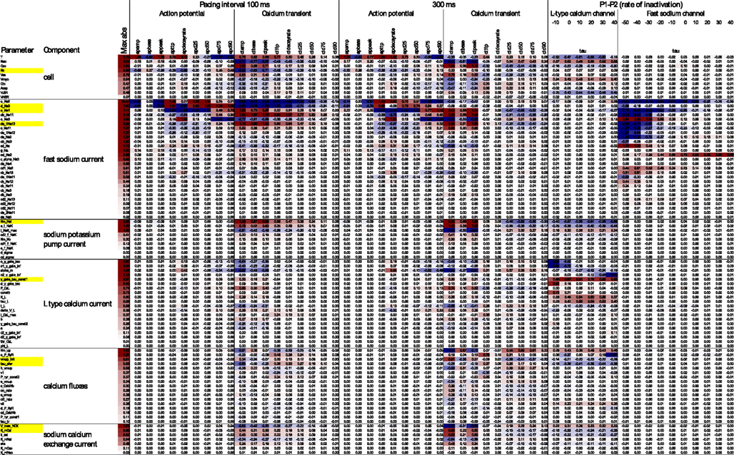
Figure 4. Elasticities and sensitivities of phenotypes (columns) with respect to parameters (rows) for selected components and phenotypes. The body of the table shows the change in phenotype per change in parameter (red = positive, blue = negative), expressed as percent (for ratio–scale quantities) or millivolt (for base and peak voltage, and voltage offset parameters). Parameters are ordered within components by their highest absolute elasticity with respect to any phenotype. See Supplementary Material for the full table, annotated with physical units, baseline values, and whether quantities were considered on relative or absolute scale.

Figure 4 demonstrates the importance of virtual experiments in model validation (see also Cooper et al., 2011). Many effects manifested more clearly in voltage-stepping experiments than under regular pacing, or under fast vs. slow pacing. Thus, genetic parameter variation that would otherwise go unnoticed can be detected by confronting model predictions with experimental data for a range of experimental protocols.

Raw Phenotypic Variability

Based on the elasticity analysis above, we selected 10 parameters exemplifying various components and influencing various phenotypes (Figure 1; Table 1), and assumed that each was determined by one biallelic locus, with genotypic values of aa = 50%, Aa = 100%, and AA = 150% of the baseline parameter estimate, for a total of 3¹⁰ = 59049 parameter scenarios. The assumption of parameter monogenicity is conservative with respect to understanding penetrance and polygenicity, and simplifies the presentation of results while not influencing the major conclusions that follow.

The simulated heart cell dynamics converged without alternans in 56%, 62%, and 65% of cases for pacing intervals of 100, 200, and 300 ms. The genotypic scenarios that did converge showed considerable phenotypic variation in action potentials, calcium transients, and ion currents under voltage-stepping (Figure 5). Action potentials clustered into a few distinct shapes, whereas the calcium transient showed more continuous phenotypic variation. This may suggest a more polygenic basis for the latter, in that a greater number of processes affect the calcium transient. The voltage-clamp experiment for the baseline scenario showed the usual short-lived current that is cut short by inactivation of ion channels (third panel, red curve in Figure 5). However, in a high proportion of genotypic scenarios the channel failed to inactivate, causing a persistent current throughout the first pulse. As a consequence, the aggregate phenotype of a time-scale of inactivation (τ) was not well defined in these cases. In summary, a cGP model generates phenotypic data that can be directly confronted with empirical measurements, giving a causal account of genetic concepts such as penetrance, dominance, and epistasis. Below we exemplify how the data can be aggregated for purposes of analysis and interpretation.

FIGURE 5

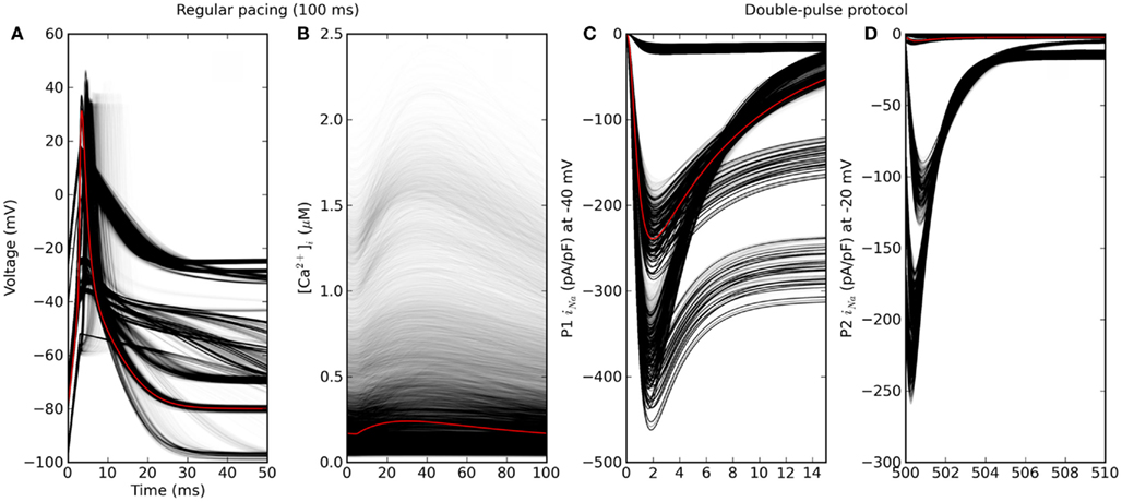
Figure 5. Phenotypic variability simulated by varying in silico genes that each determine one model parameter. Red is the baseline genotype. (A) Action potential and (B) calcium transient under regular pacing at 100 ms intervals. Only genotypes for which dynamics converged without alternans are shown (about 56% of 3¹⁰ = 59049 cases). (C,D) Fast sodium current under a double-pulse voltage-clamp experiment. Note that the time axes are truncated.

Phenotypic Correlations

Scatterplots are useful in visualizing the covariation between pairs of scalar phenotypes (cf. Figure 2) that results from simulated genetic variation (Figure 6). The distinct AP shapes in Figure 5 are reflected in the strong phenotypic correlation between APD25 and APD90 within distinct groups (Figure 6, upper red highlight). Variation in calcium transient phenotypes was more continuous, though often quite irregular (middle and lower red highlights).

FIGURE 6

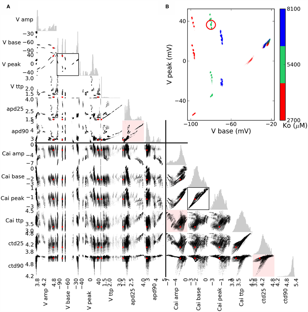
Figure 6. (A) Scatterplot matrix of bivariate phenotypic distributions for the action potential (AP) and calcium transient (CT), with univariate histograms in gray. Values are natural logarithms, except for base and peak voltage, and the lower inset. The red dot (circle in the insets) shows the baseline scenario. Red highlight: AP durations apd90 vs. apd25 exemplify fairly distinct variation in AP shape, whereas ctd90 vs. ctd25 shows more gradual variability, though the relation between amplitude and time to peak is complex. (B) Clustering of AP base and peak phenotypes exemplifies that they are affected by only a couple of simulated genes, one of which is Ko, determining the extracellular potassium concentration.

Clustering in phenotypic values may suggest that one or a few genes underlie the variation. Coloring points by genotype is informative in simple cases, for example AP peak and base vs. Ko (Figure 6, inset). However, when phenotypic ranges overlap, and multiple genotypic or other causal variation is involved, multivariate methods can give a better overview of many dependencies simultaneously, as shown below.

Characterizing a High-Dimensional Genotype-to-Phenotype Map

Partial least squares regression (Martens and Næs, 1992) provides a low-dimensional approximation of the covariance between responses (here phenotypes) and predictors (here genotypic parameters). PLS compresses both the predictors and responses into their most relevant subspaces, spanned by a basis of covariance eigenvectors (weighting each original variable by so-called loadings; scores denotes each observation’s coordinates in the new basis). The correlation between the original variables and the scores are called correlation loadings. Thus, Figure 7 places simulated loci and phenotypic measures onto a few common axes, concisely depicting their patterns of covariation.

FIGURE 7

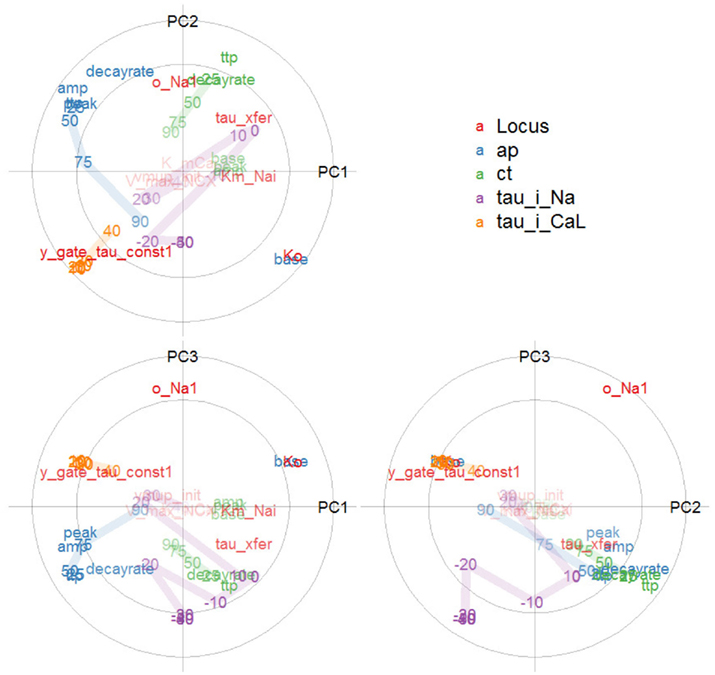
Figure 7. Overview of a multivariate genotype–phenotype map: Correlation loading plot matrix of the first three components of a partial least squares regression of action potential, calcium transient, and voltage-clamp phenotypes (categorized by color) against genotypic variables (red). The axes show correlations between a PLS component and each genotypic or phenotypic variable. The circles indicate 50 and 100% variance explained by the pair of components; labels near the center are dimmed. Variable identifiers are centered over their respective points. For the action potential (AP) and calcium transient (CT), TTP means time to peak, and lines connect the phenotypes for time to 25, 50, 75, 90% recovery. For the voltage-clamp phenotypes, lines connect the range of transmembrane voltages to which a cell was depolarized.

The placement of base voltage and other action potential phenotypes at the extremes of the PC1 axis (correlation loadings for PLS component 1) shows that these enter strongly into the first major component of phenotypic variation, as does the time-scale of the i_CaL current. The second component brings in calcium transient phenotypes. Together, the first pair of phenotypic components account almost fully (outer circle) for variation in the base voltage, whereas the variance in the calcium transient is mostly relegated to later components, in particular the combination of PC2 and PC3. The proximity of, e.g., APD25 and AP time to peak shows them to be highly correlated, whereas their being at right angles to tau_i_CaL means that these groups of phenotypes are fairly uncorrelated in this two-dimensional projection of the data. AP base is strongly negatively correlated with the other AP phenotypes, as evident from its placement opposite the others. The serial, but weakening correlation between recovery times is evident from their placement along a curve in the diagram, for both the action potential and calcium transient.

The first genotypic PLS component is dominated by Ko and y_gate_tau_const1, which are strongly correlated with the phenotypes AP base and tau_i_CaL, respectively. In summary, the PLS analysis gives a very concise depiction of the genotype-to-phenotype map, reflecting findings of both the bivariate scatterplots and variance decompositions (below).

For cases where interesting patterns apply only to subsets of the data, clustering-based methods may offer an alternative to specifying interaction terms parametrically (Tøndel et al., 2011). Many phenotypes may apply only in a portion of cases; for instance, action potential duration is well defined only if heart cell dynamics converges to stable dynamics without alternans. Such cases are amenable to a combined approach, quantifying the continuous phenotypic variation for the cases where it is well defined (Figures 7 and 9), and exploring the causes of failure using, e.g., logistic regression (Hosmer and Lemeshow, 2000).

The Genetic Basis of an in silico Disease Phenotype

We believe that defining disease phenotypes in silico holds great potential for improving understanding of different proximate causes underlying medical signs and symptoms, and of the interactions between genetic and environmental parameters that underlie epistasis and incomplete penetrance. In our study, simulated genetic variation had strong effects on the viability of in silico heart cells, as measured by their calcium handling (Figure 8). Among the genotypic scenarios that did converge, increasing the parameter d_Na3 ran the risk of reducing peak calcium to an unviable level, while reducing the voltage-sensitivity could maintain base calcium so high as to prevent proper relaxation (Figure 8). However, model dynamics failed to even converge in almost all cases for certain combinations of the genes for da_1Na13 and d_Na3, which modify the fast sodium channel’s voltage-dependency of rates of opening and recovery from inactivation, respectively (Figure 1; Table 1). The epistatic interactions between these simulated genes were not simple; gene substitutions for d_Na3 that were harmful alone could compensate for problems arising from substitutions of da_1Na13 (Figure 8), or only had an impact under stress such as fast pacing (Figure 4).

FIGURE 8

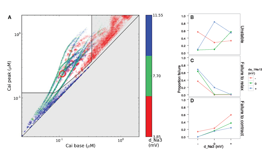
Figure 8. Simulated disease phenotype based on the calcium transient, a proxy for muscle contraction, in scenarios with stable dynamics at 200 ms pacing. (A) The gray area shows failure to contract (bottom), failure to relax (right), or insufficient calcium transient amplitude (near diagonal). Color indicates levels of d_Na3, the voltage-sensitivity of the opening rate of the fast sodium channel. (B) Interaction of d_Na3 and da_1Na13 (voltage-sensitivity of the rate of recovery from inactivation) with respect to the proportion of simulated genotypes that converged to stable dynamics. The middle and bottom panels show the proportion of stable scenarios suffering from excessive base levels of cytosolic calcium (C) or insufficient peak calcium (D).

Although simple, this example points to the possibility of classifying diseased and healthy individuals based on clinically relevant phenotypic measures, while obtaining more refined insight by analyzing the high-dimensional phenotypic variation underlying the binary classification. Highly complex interactions between genetic factors and environmental challenges may be a generic feature of complex diseases, in which case cGP models can shed light on the interplay between genetic, age-related, and lifestyle factors, based on how disease manifests at multiple phenotypic levels in a causally cohesive model.

Variance Decomposition

Traditional variance decompositions can provide helpful indications of how phenotypic variability arises from genotypic and other variation in parameters. In our study, the analysis was complicated by the fact that AP and CT phenotypes were not well defined in cases of alternans (Figure 8). For simplicity, we contrasted variance decompositions for two well-behaved subsets of the data, namely baseline and low d_Na3 at baseline values of da_1Na13. We fitted linear regression models (function lm in R) for each scalar measure of the action potential and calcium transient, with genotypic variables as predictors, including second-order interactions and quadratic terms. In the resulting variance decompositions (Figure 9), phenotypes ranged from being monogenic to oligogenic to polygenic, even under the conservative assumption that low-level parameters were strictly monogenic.

FIGURE 9

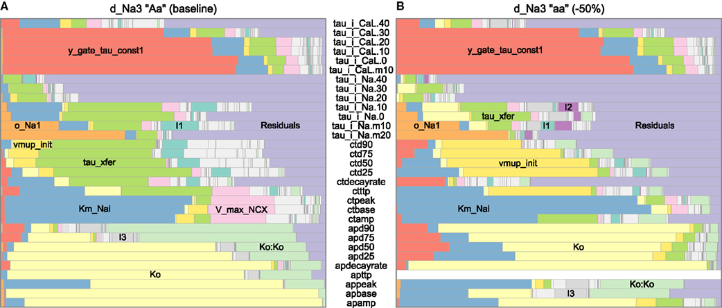
Figure 9. Effect of a hypothetical gene (d_Na3) on variance decompositions of action potential (AP), calcium transient (CT), and voltage-clamp (VT) phenotypes, based on linear regression against genotypic parameters including second-order and quadratic terms to capture genetic interactions and intralocus non-additivity. Simulated genes with large variance components are labeled; Ko:Ko denotes the quadratic term for Ko. Second-order interactions were minor in this case except those of tau_xfer and Km_Nai (labeled I1), tau_xfer and Ko (I2), Km_Nai and Ko (I3), or tau_xfer and vmup_init (I4). Higher-order terms are lumped in “Residuals.” Voltage-clamp phenotypes include the characteristic time-scale (tau) for the L-type calcium and fast sodium currents after a step depolarization (e.g., to −50 mV for tau_i_Na.m50). To restrict the illustration to well-behaved subsets of the data, only scenarios with baseline (A) or low (B) levels of d_Na3, baseline levels of da_1Na13, and a stimulus period of 200 ms (for AP and CT) are shown.

Figure 9 illustrates the potential of cGP models in systematically assessing the degree to which the –genicity of complex traits and associated penetrance patterns are likely to change as a function of the genetic background. Action potential phenotypes appeared largely monogenic (due to Ko, with very non-additive effects, e.g., on APD90) at baseline d_Na3, but di- or trigenic at low d_Na3. The AP amplitude and early-stage AP duration varied by Km_Nai (in the sodium–potassium pump component), whereas AP durations were also influenced by y_gate_tau_const1 (in the L-type calcium current component). (AP time to peak had zero variability at low d_Na3, because repolarization was already underway by the end of the stimulus.) The two backgrounds showed also very different major determinants of calcium transient phenotypes. Under baseline d_Na3, the greatest variance component was due to tau_xfer (affecting calcium release from subspace to cytosol), whereas vmup_init (affecting calcium re-uptake from cytosol) dominated at low d_Na3. These results suggest that varying –genicity and penetrance may be generic features of complex physiological traits, and that these features can be systematically and meaningfully studied by use of cGP models.

For example, findings of quantitative trait loci (QTLs) underlying complex traits are often not consistent across populations (Beavis, 1998). cGP models may shed light on whether QTLs for variation in lower-level processes are likely to manifest in higher-level phenotypes and to assess the associated penetrance characteristics, informing the interpretation of empirical data and guiding experimental search for putative QTLs.

Parameters are Phenotypes

From the assumption that low-level parameters were strictly monogenic, emerged a polygenic basis for phenotypes such as the characteristic time-scale of ion channels; phenotypes that might be used as parameters in more aggregate models (Rajasingh et al., 2008). Similarly, many parameters that we assumed monogenic and constant could instead be derived from mechanistic submodels. For instance, the output of gene regulatory models for the expression levels of ion transport proteins corresponds directly to model parameters that scale ion currents, such as V_max_NCX or vmup_init in Table 1 (see, e.g., Gjuvsland et al., 2006) An example of gene regulatory responses was seen with conditional knockout of the SERCA channel, which was partially compensated for by increased expression of other calcium channels (Andersson et al., 2009). Modeling signal transduction and gene regulation (Cooling et al., 2009), electromechanical coupling (Niederer and Smith, 2007) and whole-organ phenomena (Nordsletten et al., 2011) are further promising targets for realistic gene-to-parameter mapping in cGP modeling. The requisite data and tools are just becoming available through databases, coding standards, and ontologies such as those promoted by the Physiome Project (Hunter and Borg, 2003) and the Virtual Physiological Human (Hunter et al., 2010). For example, the knowledge in genomic and phenomic databases can become vastly more usable through annotation with biologically meaningful, yet machine-processable descriptors. Phenotypic assays can be linked to models by complementing model repositories (Le Novere et al., 2006; Lloyd et al., 2008) with simulation experiment descriptions in appropriate languages (Köhn and Novère, 2011).

Concluding Remarks

In their commentary entitled “Life after GWA studies,” Dermitzakis and Clark (2009) conclude that “A major breakthrough will be to predict and interpret the effect of mutational and biochemical changes in human cells and understand how this signal is transmitted spatially (among tissues) and temporally (spanning development).” Causally cGP modeling addresses exactly this vision by bridging the gap between genomic information and the high-dimensional phenotypes of individuals. The physiologically validated cell model in our case study exhibits many well-known genetic phenomena such as variable penetrance of a binary disease phenotype, intralocus dominance, non-linear responses, interlocus epistasis, varying degrees of phenotypic correlation (Figure 6), and a range from monogenic to oligo- and polygenic traits (Figure 9). Thus, model results are amenable both to standard quantitative genetic methods (Lynch and Walsh, 1998) and novel applications of high-dimensional data analysis (Martens and Næs, 1992). The close parallel between empirical and cGP studies makes for a tight link to experimental work (cf. Figure 3). Whereas passive observation may not provide the most informative phenotypes, experiments (real and virtual) can be designed to bring into play system components whose importance manifests only under certain conditions or perturbations. Because the parameter-to-phenotype model is based on physiological principles and empirical data (Hunter and Borg, 2003), a cGP study generates experimentally verifiable hypotheses for both physiological and genetic studies at multiple phenotypic levels (Rajasingh et al., 2008) in a way that statistical-genetic studies cannot (Dermitzakis and Clark, 2009). In personalized medicine, this approach can lead toward a systemic understanding of what it takes to force a diseased system into a healthier state. Incorporating the effects of environmental and lifestyle variation on parameters and phenotypes is an important next step. A computational physiological genomics will have to involve a whole range of theoretical methodologies and approaches, but we find it hard to envisage how we can achieve a deep understanding of the genotype–phenotype relationship without letting cGP modeling become a key element in this emerging discipline.

Conflict of Interest Statement

The authors declare that the research was conducted in the absence of any commercial or financial relationships that could be construed as a potential conflict of interest.

Acknowledgments

This work was funded by the Research Council of Norway under the eVITA programme, project number 178901/V30. NOTUR, the Norwegian metacenter for computational science, provided computing resources under project nn4653k. We are grateful to Johan Hake for help in getting acquainted with the Bondarenko model.

Supplementary Material

The Supplementary Material for this article can be found online at http://www.frontiersin.org/Genomic_Physiology_/10.3389/fphys.2011.00106/abstract

Footnotes

1. ^http://lxml.de
2. ^www.python.org

References

Andersson, K. B., Birkeland, J. A. K., Finsen, A. V., Louch, W. E., Sjaastad, I., Wang, Y., Chen, J., Molkentin, J. D., Chien, K. R., Sejersted, O. M., and Christensen, G. (2009). Moderate heart dysfunction in mice with inducible cardiomyocyte-specific excision of the Serca2 gene. J. Mol. Cell. Cardiol. 47, 180–187.

Pubmed Abstract | Pubmed Full Text | CrossRef Full Text

Bateson, W. (1906). “The progress of genetic research: an inaugural address to the third conference on hybridisation and plant-breeding,” in Scientific Papers of William Bateson (1928), ed. R. S. Punett (Cambridge: University Press), 142–151.

Beavis, W. D. (1998). “QTL analyses: power, precision, and accuracy,” in Molecular Dissection of Complex Traits, ed. A. H. Paterson (Boca Raton, FL: CRC Press), 145–162.

Bondarenko, V. E., Szigeti, G. P., Bett, G. C. L., Kim, S.-J., and Rasmusson, R. L. (2004). Computer model of action potential of mouse ventricular myocytes. Am. J. Physiol. Heart Circ. Physiol. 287, H1378–H1403.

Pubmed Abstract | Pubmed Full Text | CrossRef Full Text

Burns, J. (1970). “The synthetic problem and the genotype-phenotype relation in cellular metabolism,” in Towards a Theoretical Biology. 3. Drafts. An I.U.B.S. Symposium, ed. C. H. Waddington (Chicago: Aldine Publishing Company), 47–51.

Cohen, S. D., and Hindmarsh, A. C. (1996). CVODE, a stiff/nonstiff ODE solver in C. Comput. Phys. 10, 138–143.

Cooling, M. T., Hunter, P., and Crampin, E. J. (2009). Sensitivity of NFAT cycling to cytosolic calcium concentration: implications for hypertrophic signals in cardiac myocytes. Biophys. J. 96, 2095–2104.

Pubmed Abstract | Pubmed Full Text | CrossRef Full Text

Cooper, J., Mirams, G. R., and Niederer, S. A. (2011). High-throughput functional curation of cellular electrophysiology models. Prog. Biophys. Mol. Biol. 107, 11–20.

Pubmed Abstract | Pubmed Full Text | CrossRef Full Text

Dermitzakis, E. T., and Clark, A. G. (2009). Life after GWA studies. Science 326, 239–240.

Pubmed Abstract | Pubmed Full Text | CrossRef Full Text

Falconer, D. S., and Mackay, T. F. C. (1996). Introduction to Quantitative Genetics. 4th Edn. Harlow: Longman Group.

Gilchrist, M. A., and Nijhout, H. F. (2001). Nonlinear developmental processes as sources of dominance. Genetics 159, 423–432.

Pubmed Abstract | Pubmed Full Text

Gjuvsland, A., Hayes, B., Meuwissen, T., Plahte, E., and Omholt, S. (2007a). Nonlinear regulation enhances the phenotypic expression of trans-acting genetic polymorphisms. BMC Syst. Biol. 1, 32. doi: 10.1186/1752-0509-1-32

CrossRef Full Text

Gjuvsland, A., Plahte, E., and Omholt, S. (2007b). Threshold-dominated regulation hides genetic variation in gene expression networks. BMC Syst. Biol. 1, 57. doi: 10.1186/1752-0509-1-57

CrossRef Full Text

Gjuvsland, A. B., Hayes, B. J., Omholt, S. W., and Carlborg, O. (2007c). Statistical epistasis is a generic feature of gene regulatory networks. Genetics 175, 411–420.

CrossRef Full Text

Gjuvsland, A. B., Hayes, B. J., Omholt, S. W., and Carlborg, O. (2006). Statistical epistasis is a generic feature of gene regulatory networks. Genetics 175, 411–420.

Pubmed Abstract | Pubmed Full Text | CrossRef Full Text

Gjuvsland, A. B., Plahte, E., Ådnøy, T., and Omholt, S. W. (2010). Allele interaction – single locus genetics meets regulatory biology. PLoS ONE 5, e9379. doi: 10.1371/journal.pone.0009379

CrossRef Full Text

Hancock, J. M., Mallon, A.-M., Beck, T., Gkoutos, G. V., Mungall, C., and Schofield, P. N. (2009). Mouse, man, and meaning: bridging the semantics of mouse phenotype and human disease. Mamm. Genome 20, 457–461.

Pubmed Abstract | Pubmed Full Text | CrossRef Full Text

Hosmer, D. W., and Lemeshow, S. (2000). Applied logistic Regression, 2nd Edn. New York: Wiley.

Hund, T. J., Kucera, J. P., Otani, N. F., and Rudy, Y. (2001). Ionic charge conservation and long-term steady state in the Luo–Rudy dynamic cell model. Biophys. J. 81, 3324–3331.

Pubmed Abstract | Pubmed Full Text | CrossRef Full Text

Hunter, P., Coveney, P. V., de Bono, B., Diaz, V., Fenner, J., Frangi, A. F., Harris, P., Hose, R., Kohl, P., Lawford, P., McCormack, K., Mendes, M., Omholt, S., Quarteroni, A., Skår, J., Tegner, J., Randall Thomas, S., Tollis, I., Tsamardinos, I., van Beek, J. H. G. M., and Viceconti, M. (2010). A vision and strategy for the virtual physiological human in 2010 and beyond. Philos. Transact. A Math. Phys. Eng. Sci. 368, 2595–2614.

Pubmed Abstract | Pubmed Full Text | CrossRef Full Text

Hunter, P. J., and Borg, T. K. (2003). Integration from proteins to organs: the physiome project. Nat. Rev. Mol. Cell Biol. 4, 237–243.

Pubmed Abstract | Pubmed Full Text | CrossRef Full Text

Köhn, D., and Novère, N. (2011). “SED-ML – an XML format for the implementation of the MIASE guidelines [online],” in Computational Methods in Systems Biology, eds M. Heiner, and A. M. Uhrmacher (Berlin: Springer Berlin Heidelberg), 176–190.

Langtangen, H. P. (2009). Python Scripting for Computational Science, 3rd Edn. Berlin: Springer Berlin Heidelberg.

Le Novere, N., Bornstein, B., Broicher, A., Courtot, M., Donizelli, M., Dharuri, H., Li, L., Sauro, H., Schilstra, M., Shapiro, B., Snoep, J. L., and Hucka, M. (2006). BioModels database: a free, centralized database of curated, published, quantitative kinetic models of biochemical and cellular systems. Nucl. Acids Res. 34, D689–D691.

CrossRef Full Text

Li, L., Niederer, S. A., Idigo, W., Zhang, Y. H., Swietach, P., Casadei, B., and Smith, N. P. (2010). A mathematical model of the murine ventricular myocyte: a data-driven biophysically based approach applied to mice overexpressing the canine NCX isoform. Am. J. Physiol. Heart Circ. Physiol. 299, H1045–H1063.

Pubmed Abstract | Pubmed Full Text | CrossRef Full Text

Lloyd, C. M., Halstead, M. D., and Nielsen, P. F. (2004). CellML: its future, present and past. Prog. Biophys. Mol. Biol. 85, 433–450.

Pubmed Abstract | Pubmed Full Text | CrossRef Full Text

Lloyd, C. M., Lawson, J. R., Hunter, P. J., and Nielsen, P. F. (2008). The cellML model repository. Bioinformatics 24, 2122–2123.

Pubmed Abstract | Pubmed Full Text | CrossRef Full Text

Lynch, M., and Walsh, B. (1998). Genetics and Analysis of Quantitative Traits, 1st Edn. Sunderland: Sinauer Associates.

Martens, H., and Næs, T. (1992). Multivariate Calibration. 1st Edn. Chichester: Wiley.

Martens, H., Veflingstad, S., Plahte, E., Martens, M., Bertrand, D., and Omholt, S. (2009). The genotype-phenotype relationship in multicellular pattern-generating models – the neglected role of pattern descriptors. BMC Syst. Biol. 3, 87. doi: 10.1186/1752-0509-3-87

CrossRef Full Text

Mevik, B. H., and Wehrens, R. (2007). The pls package: principal component and partial least squares regression in R. J. Stat. Softw. 18, 1–24.

Molleman, A. (2002). Patch Clamping: An Introductory Guide to Patch Clamp Electrophysiology, 1st Edn. New York, NY: Wiley.

Niederer, S. A., Fink, M., Noble, D., and Smith, N. P. (2008). A meta-analysis of cardiac electrophysiology computational models. Exp. Physiol. 94, 486–495.

CrossRef Full Text

Niederer, S. A., and Smith, N. P. (2007). An improved numerical method for strong coupling of excitation and contraction models in the heart. Prog. Biophys. Mol. Biol. 96, 90–111.

Pubmed Abstract | Pubmed Full Text | CrossRef Full Text

Noble, D. (2002a). Modeling the heart – from genes to cells to the whole organ. Science 295, 1678–1682.

CrossRef Full Text

Noble, D. (2002b). The rise of computational biology. Nat. Rev. Mol. Cell Biol. 3, 459–463.

CrossRef Full Text

Nordsletten, D. A., Niederer, S. A., Nash, M. P., Hunter, P. J., and Smith, N. P. (2011). Coupling multi-physics models to cardiac mechanics. Prog. Biophys. Mol. Biol. 104, 77–88.

Pubmed Abstract | Pubmed Full Text | CrossRef Full Text

Oliphant, T. E. (2006). Guide to NumPy. Spanish Fork, UT: Trelgol Publishing.

Omholt, S. W., Plahte, E., Oyehaug, L., and Xiang, K. (2000). Gene regulatory networks generating the phenomena of additivity, dominance and epistasis. Genetics 155, 969–980.

Pubmed Abstract | Pubmed Full Text

Peccoud, J., Velden, K. V., Podlich, D., Winkler, C., Arthur, L., and Cooper, M. (2004). The selective values of alleles in a molecular network model are context dependent. Genetics 166, 1715–1725.

Pubmed Abstract | Pubmed Full Text | CrossRef Full Text

R Development Core Team. (2011). R: A language and environment for statistical computing. Vienna: Foundation for Statistical Computing.

Rajasingh, H., Gjuvsland, A. B., Våge, D. I., and Omholt, S. W. (2008). When parameters in dynamic models become phenotypes: a case study on flesh pigmentation in the chinook salmon (Oncorhynchus tshawytscha). Genetics 179, 1113–1118.

Pubmed Abstract | Pubmed Full Text | CrossRef Full Text

Roberts, R., and Brugada, R. (2003). Genetics and Arrhythmias. Annu. Rev. Med. 54, 257–267.

Pubmed Abstract | Pubmed Full Text | CrossRef Full Text

Roepke, T. K., and Abbott, G. W. (2006). Pharmacogenetics and cardiac ion channels. Vascul. Pharmacol. 44, 90–106.

Pubmed Abstract | Pubmed Full Text | CrossRef Full Text

Sanguinetti, M. C., and Tristani-Firouzi, M. (2006). hERG potassium channels and cardiac arrhythmia. Nature 440, 463–469.

Pubmed Abstract | Pubmed Full Text | CrossRef Full Text

Tøndel, K., Indahl, U., Gjuvsland, A. B., Vik, J. O., Hunter, P. J., Omholt, S. W., and Martens, H. (2011). Hierarchical Cluster-Based Partial Least Squares Regression (HC-PLSR) is an efficient tool for metamodelling of nonlinear dynamic models. BMC Syst. Biol. 5, 90ff. doi: 10.1186/1752-0509-5-90

CrossRef Full Text

Welch, S. M., Dong, Z. S., Roe, J. L., and Das, S. (2005). Flowering time control: gene network modelling and the link to quantitative genetics. Aust. J. Agric. Res. 56, 919–936.

CrossRef Full Text

Wickham, H. (2009). ggplot2: Elegant Graphics for Data Analysis, 1st Edn. New York, NY: Springer.

Wikipedia. (2010). Design pattern (computer science) [Online]. Wikipedia, The Free Encyclopedia Wikimedia Foundation. Available at: http://en.wikipedia.org/w/index.php?title=Design_pattern_(computer_science)&oldid=378971385 [accessed 17 August 2010].