The Conundrum of Functional Brain Networks: Small-World Efficiency or Fractal Modularity

The human brain has been studied at multiple scales, from neurons, circuits, areas with well-defined anatomical and functional boundaries, to large-scale functional networks which mediate coherent cognition. In a recent work, we addressed the problem of the hierarchical organization in the brain through network analysis. Our analysis identified functional brain modules of fractal structure that were inter-connected in a small-world topology. Here, we provide more details on the use of network science tools to elaborate on this behavior. We indicate the importance of using percolation theory to highlight the modular character of the functional brain network. These modules present a fractal, self-similar topology, identified through fractal network methods. When we lower the threshold of correlations to include weaker ties, the network as a whole assumes a small-world character. These weak ties are organized precisely as predicted by theory maximizing information transfer with minimal wiring costs.

1. Introduction

The functional magnetic resonance imaging (fMRI) technique is a tool that has greatly improved our ability to probe brain activity. The method detects changes in blood oxygenation when areas of the brain are activated and consequently require increased blood flow. In this way, we can monitor what brain areas respond to different mental activities. The resulting datasets offer a three-dimensional image of the brain indicating the level of activation at various regimes.

Many methods have been applied to analyze fMRI data, ranging from statistics to signal processing techniques. Recently, the brain organization has been described as a complex network (Eguiluz et al., 2005; Sporns et al., 2005; Bullmore and Sporns, 2009). This approach can take various forms, such as physical connections between neurons or correlations in the activity between brain areas at a coarser level. In a recent work (Gallos et al., 2012) we used recent advances in fractal network theory to characterize the brain clusters structure, and studied one key problem of neuroscience, namely the integration of modular clusters in a larger scale. Here, we expand on those findings and describe the methodology in detail, focusing on the use of network theory in the study of fMRI data.

One of the main features of our sensations is its unitary nature. The brain can receive many concurrent stimuli. These have to be processed independently of each other, but at the same time they have to be integrated into a unified entity. This suggests that the modalities in the brain that process different characteristics have to act isolated for efficient computations, but they need also be sufficiently connected in order to perform coherent functions.

The notion of a complex network can be suitably adapted to address this scaling problem and study optimal information flow in modular networks. This representation of complicated interactions has offered new insight in many processes across different disciplines. A key feature of many such networks is their modular character, a topic which has attracted a lot of interest in the literature. Many algorithms have been proposed for the detection of modules, loosely defined as network areas well-connected within themselves but sparsely connected to the rest of the network. The detection and behavior of modules at different observation scales, though, remains a largely unexplored problem. Network analysis of functional (Eguiluz et al., 2005) and structural (Sporns et al., 2005) data has been used to characterize global connectivity and topological organization of the human brain (Bullmore and Sporns, 2009). Many of those studies indicate the small-world character (Watts and Strogatz, 1998) of brain networks, but the idea of a simple small-world structure can be contradictory to modular network.

In the present manuscript we implement a complex network analysis to understand the hierarchical organization of functional brain networks, and we study how we can explain the emergence of both small-world and modular features in the same network. We capitalize on a well known dual-task paradigm, the psychological refractory period, in which information from different sensory modalities (visual and auditory) has to be coherently routed to different motor effectors (in this experiment, the left and right-hand).

The combination of high-temporal resolution fMRI with novel network analysis tools allows the study of the module properties and their synergy toward accomplishing a cognitive task. A functional correlation network is derived from the fMRI phase information. We implement percolation and scaling analysis methods to uncover a highly modular functional operation and a network that is almost optimally connected for efficient information flow.

2. Materials and Methods

2.1. Experimental Design

We use time-resolved fMRI (Menon et al., 1998), based on analysis of the phase signal (Sigman et al., 2007). Time-resolved fMRI is capable of identifying the series of processing stages which unfold sequentially during the execution of a compound dual-task (Dux et al., 2006; Sigman and Dehaene, 2008).

The details of the experiments are described in Sigman et al. (2007), and are briefly reviewed here. Sixteen participants performed a dual-task paradigm: first a visual task of comparing an Arabic numeral (target T1) to a fixed reference, with a right-hand response and, second, an auditory task of judging the pitch of an auditory tone (target T2) with a left-hand response. The stimulus onset asynchrony (SOA) between T1 and T2 was varied between 0, 300, 900, and 1200 ms. In the course of this analysis we did not detect significant differences in the resulting patterns of different SOA conditions.

While subjects performed the dual-task, whole-brain fMRI images were recorded at a sampling time (TR) of 1.5 s, and subsequently the phase and amplitude of the hemodynamic response were computed (Sigman et al., 2007). This activated map exhibits phases consistently falling within the expected response latency for a task-induced activation. As expected for an experiment involving visual and auditory stimuli and bimanual responses, the responsive regions included bilateral visual occipito-temporal cortices, bilateral auditory cortices, motor, premotor and cerebellar cortices, and a large-scale bilateral parieto-frontal network (Sigman and Dehaene, 2008). In this study we try to understand the topology of the modular organization of this broad functional network during dual-task performance. For this purpose, we derived a large functional network of brain areas by measuring the phase correlations in these responses for all pairs of voxels. We then connected the highly correlated pairs which gave us the brain cluster network structure.

2.2. Phase Correlations and Functional Brain Network

We use network theory concepts for the analysis of correlations between different brain areas, based on the temporal activation of these areas when a subject responds to external stimuli. We reconstruct the network topology of brain voxels, where a network link indicates a high correlation in the phase-space activity of the two connected voxels, and compare this structure with the corresponding topology of the voxel location in the brain.

The time evolution of the phase of all brain voxels over 440 s was recorded for each participant and each of the four SOA conditions, for a total of 64 measurements. For our analysis, we create a mask where we only keep voxels which were activated in more than 75% of the cases, i.e., in at least 48 instances.

We want to detect the correlation between the phases of two voxels i and j in the activated mask. The measure of correlation for vectors is the co-directionality, i.e., we need to calculate the angle between the two vectors. Therefore, the correlation c_ij between two vectors ${\overrightarrow{r}}_i$ and ${\overrightarrow{r}}_j$ is given, in general, by $c_{ij}\equiv {\overrightarrow{r}}_i\cdot {\overrightarrow{r}}_j∕\left|{\overrightarrow{r}}_i\right|\left|{\overrightarrow{r}}_j\right|,$ which is equivalent to the cosine of the included angle, i.e., c_ij = cos(θ), where θ is now the phase difference a_i − a_j. We average the correlation between any two voxels i and j in the activated mask over roughly 40 trials of each experiment. The resulting correlation p_ij between these two voxels is then given by

$p_{ij}=\frac{1}{N}\sum _{t=1}^{N}cos\left[a_i\left(t\right)-a_j\left(t\right)\right],$(1)

where N is the number of trials for a given combination of subject and stimulus. We link two voxels if their correlation is larger than a threshold value p. The resulting network is a representation of functional relations among voxels for a specific subject and stimulus.

The topology of this network strongly depends on the value of p. The variation of p describes a percolation process. A large p-value enables isolated module identification, since only the strongest (i.e., more correlated) functional links between voxels are preserved. As p is lowered, these modules get progressively merged to larger entities and the emphasis is shifted toward large-scale properties of the spanning network.

The complex network representation (Figure 1A) reveals functional links between brain areas, but cannot directly reveal spatial correlations. Since voxels are embedded in space, we also study the topological features of spatial clusters in three-dimensions, where now voxels assume their known positions in the brain and links between them are transferred from the corresponding network (Figure 1B), i.e., they are assigned according to the degree of correlation between any two voxels, independently of the voxels proximity in real-space.

FIGURE 1

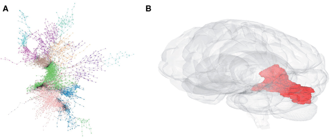
Figure 1. (A) Network representation of a brain cluster, as found by the phase correlation between pairs of voxels. (B) The same cluster in real-space representation, where each voxel is now placed in its known location in the brain.

The above procedure yields a different network or spatial clusters for each subject. We study each of those networks and clusters separately and show that they all carry statistically similar properties. For efficiency purposes, we focus our attention to the case of the largest p_c value where three clusters, including at least 1000 voxels, emerge in each trial. The spread of the corresponding p_c values is small, demonstrating a similar behavior in the brain response of different subjects.

2.3. Fractal Analysis

We analyze the resulting networks and the embedded three-dimensional clusters in terms of their fractal and modular properties. For the spatial representation, we characterize the fractality of a connected cluster through the standard Hausdorff dimension d_f. Starting from an arbitrary point in a cluster, d_f measures how the mass N_f (number of voxels in the same cluster) scales with the Euclidean distance r from this origin, i.e.:

$N_f\left(r\right)\sim r^{d_f}.$(2)

The exponent d_f shows how densely the area is covered by a specific cluster.

The box-covering technique is used for the fractal analysis of the complex networks. A network (in our case each cluster) is first tiled with the minimum possible number of boxes, N_B, of a given size ℓ_B. A box is defined as a union of nodes, all of which are at a distance from each other smaller than a given threshold length, the box size ℓ_B (the distance between two nodes, ℓ, is defined as the number of links along the shortest path between those nodes in the functional brain network).

The fractality (self-similarity) of the network is quantified in the power-law relation between the number of boxes needed to cover the network and the box size ℓ_B:

$N_B\left({\ell }_B\right)=N_0{\ell }_B^{-d_B},$(3)

where d_B is the fractal dimension (or box dimension) and N₀ is the number of nodes in the original network (Song et al., 2005a, 2006; Goh et al., 2006; Kim et al., 2007; Radicchi et al., 2008). Finite and small values of d_B show that the network has fractal features, where the covering boxes retain their connectivity scheme under different scales, and larger-scale boxes behave in a similar way as the original network.

The requirement that the number of boxes should be minimized poses an optimization problem which can be solved using a number of box-covering algorithms. The method that we implement here is called Maximum Excluded Mass Burning algorithm (MEMB), and the algorithm can be downloaded from http://lev.ccny.cuny.edu/hmakse/soft_data.html). The method is roughly explained in Figure 2. The detection of modules or boxes in our work follows from the application of this algorithm (Song et al., 2005a, 2007) at different length-scales.

FIGURE 2

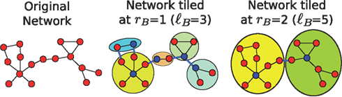
Figure 2. Demonstration of the MEMB box-covering algorithm. For a given radius value, e.g., r_B = 1 in the center panel and r_B = 2 in the right panel, we cover the network with the smallest possible number of boxes. The diameter of the box, ℓ_B (i.e., the distance between any two nodes in a box) is defined as ℓ_B = 2r_B + 1. First, we detect the smallest possible number of box origins (shown with blue color) that provide the maximum number of nodes (mass) in each box, according to an optimization algorithm described in Song et al. (2007). Then, we build the boxes through simultaneous burning from these center nodes, until the entire network is covered with boxes. For the calculation of modularity, we consider the boxes at each r_B value as separate modules. Then we calculate the ratio between the number of links within the modules (black links) and the number of links between modules (blue links).

The MEMB method starts by determining the minimum number of boxes of radius r_B required for a complete coverage of the network. This radius is the distance from a box “center,” so that by definition all nodes in a box are within a distance from each other smaller than ℓ_B = 2r_B + 1. The method detects the nodes that will act as the centers of the boxes, by calculating the mass around each node if it would act as a center. The node with maximum mass around it is selected as a center and we proceed iteratively to find the minimum number of such centers. Once these nodes have been determined, the boxes are built by including successive layers of nodes around the centers. The details of the method are reported in Song et al. (2007).

The resulting boxes are characterized by the proximity between all their nodes, at a given length-scale and the maximization of the mass associated with each module center. Thus, MEMB detects boxes that also tend to maximize modularity. Different values of the box diameter ℓ_B yield boxes of different size. These boxes are then identified as modules which at a smaller scale ℓ_B may be separated, but merge into larger entities as we increase ℓ_B. Thus, we can study the hierarchical character of modularity, i.e., modules of modules, and we can detect whether modularity is a feature of the network that remains scale-invariant.

For this, we can extend the box-covering concept to act as a community detection algorithm (Galvao et al., 2010). MEMB identifies modules of size ℓ_B, composed of highly connected brain areas. Typical modularity approaches do not place constraints on the size of the modules, but they focus on minimizing the number of inter-module links. The MEMB approach, though, has the additional advantage that modularity can be studied at different scales. The requirement of minimal number of modules to cover the network (N_B) guarantees that the partition of the network is such that each module contains the largest possible number of nodes and links inside the module with the constraint that the modules cannot exceed size ℓ_B. This optimized tiling process gives rise to modules with the fewest number of links connecting to other modules. This implies that the degree of modularity for a given ℓ_B value is maximized, and we can define a modularity measure, ℳ through (Newman and Girvan, 2004; Guimerà and Amaral, 2005; Caldarelli and Vespignani, 2007; Gallos et al., 2007)

$\mathcal{ℳ}\left(\ell \right)\equiv \frac{1}{N_B}\sum _{i=1}^{N_B}\frac{L_i^{\text{in}}}{L_i^{\text{out}}}.$(4)

Here $L_i^{\text{in}}$ and $L_i^{\text{out}}$ represent the number of links that start in a given module i and end either within or outside i, respectively. Large values of ℳ (i.e., $L_i^{\text{out}}\to 0$) correspond to a higher degree of modularity (Gallos et al., 2007).

The value of the modularity of the network ℳ varies with ℓ_B, so that we can detect the dependence of modularity on different length-scales, or equivalently how the modules themselves are organized into larger modules that enhance the degree of modularity. In the case that the dependence has a power-law form, we can define a modularity exponent d_M, through the relation:

$\mathcal{ℳ}\left({\ell }_B\right){\ell }_B^{d_M}.$(5)

3. Results

3.1. Percolation Analysis Reveals the Modular Structure

We use percolation theory (Bunde and Havlin, 1996) to identify the functional clusters resulting from the correlation between the phases of two voxels. The percolation problem is a paradigm of critical phase transitions (Stanley, 1971; Vicsek, 1992) which can be used to identify the functional clusters in the brain network. In the simplest version of percolation, we can consider a lattice where each bond is absent with probability p or present with probability 1 − p (Bunde and Havlin, 1996). In lattices, it is well known that there exists a critical probability p_c, below which the largest cluster of connected bonds spans the whole length of the lattice, while for p > p_c only small isolated clusters survive.

In the case of the functional brain network, the corresponding probability p for the existence of a link between any two voxels in the brain is based on the value of the phase correlation between them. For each participant, we calculated the mass of the largest cluster as a function of the percolation threshold p. As explained above, in a broad variety of systems in nature, the size of the largest cluster in a percolation process remains very small and increases abruptly through a phase transition, in which a single largest cluster spans the whole system (Bunde and Havlin, 1996). A single incipient cluster is expected to appear if the bonds in the network are occupied at random without correlations, i.e., when the probability to find an active bond is independent on the activity of all the other bonds in the network. For the functional brain network our results revealed a more complex picture.

We found that, for all participants in this study, the cluster size increased progressively with a series of sharp jumps (Figure 3) and not with a single jump as expected for the simpler picture of uncorrelated percolation. Moreover, in random percolation the second largest cluster has a strong peak around p_c and vanishes otherwise. In the brain network, the second largest cluster also increases through jumps of absorbing smaller clusters. This second cluster remains comparable in size with the largest cluster over a wider range of p. The evolution of these cluster sizes with p is a strong indication of strong correlations deviating from a random process.

FIGURE 3

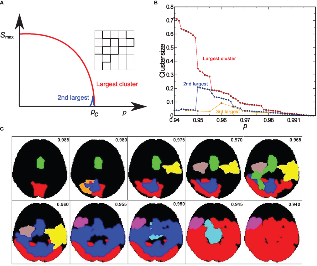
Figure 3. (A) Bond percolation in a 2-dimensional lattice. We remove a random bond with probability p, and with probability 1 − p a bond remains (denoted by a solid black line). The lattice with solid black bonds is at the percolation transition p = p_c. (B) Evolution of modules at different thresholds. The size of the three largest clusters as a function of the correlation threshold p for a given subject. As we lower p the cluster size increases in jumps, and new clusters emerge, grow, and finally get absorbed by the largest cluster. This behavior is significantly different from the random percolation in (A). (C) Cluster evolution. Brain clusters with more than 1000 voxels, as identified through correlation analysis for a given p-value.

We identified each of the jumps in the largest cluster as a single percolation transition focused on a region of the brain that is highly correlated and therefore represents a well-defined module (Figure 3). These sharp transitions are indicative of a marked modular structure in the network. They indicate that at any given p-value there are many isolated clusters in the brain network, which subsequently merge into the largest cluster as p decreases. This is a universal behavior observed in all participants, and allows the identification of functional modules, which we proceed to study next.

The clusters identified by percolation analysis at a given threshold p are functionally connected, but the nodes in such a cluster are not necessarily clustered in space. Thus, we first studied whether the percolation clusters had a consistent spatial projection. The p-values at which clusters appear varied across participants. To group the data, we measured, for each participant, the highest correlation p-value for which there were at least three clusters of 1000 voxels each. The topography of these clusters reflected coherent patterns across different individuals. In virtually all participants we observed a cluster covering the premotor, supplementary motor area (SMA) region, a cluster covering the medial part of the posterior parietal cortex (PPC) and a cluster covering the medial part of early retinotopic cortex (area V1), along the calcarine fissure.

We then measured the likelihood that a voxel may appear in a percolation cluster, by counting, for each voxel, the number of individuals for which it was included in one of the first three percolation clusters (Figure 4).

FIGURE 4

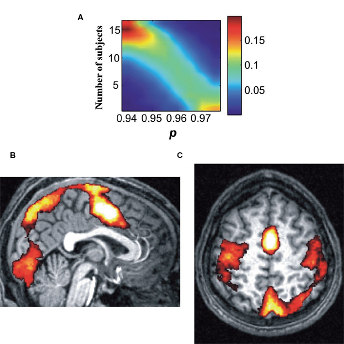
Figure 4. The emerging clusters have consistent spatial projections. (A) The color denotes the fraction of the total number of voxels that appear to one of the three largest clusters in N subjects at a given percolation threshold p. As we reduce the threshold the peak shifts toward larger N values, i.e., the same voxels appear consistently in the largest clusters for all subjects. (B,C) Spatial distribution of the first percolation clusters (in subject counts). The two brain slices show for the highest p-values the shared voxels. White bleached regions correspond to voxels which are included in the first percolation cluster for all subjects. The SMA, a region involved in planning motor action is the only shared region for all subjects.

Clusters in the three main nodes, V1, SMA, PPC, are ubiquitously present in percolation clusters and, to a lesser extent, voxels in the motor cortex (along the central sulcus) slightly more predominantly on the left hemisphere.

This analysis demonstrated that the correlation networks obtained from each subject yielded percolation clusters with consistent topographic projections. Next we focus on our main aim; exploring the topology and scaling properties of the network modules using fractal network analysis.

3.2. Fractal Analysis Results

For each of the 16 participants and each of the 4 SOA conditions we calculated the resulting network through the phase correlation. Then, for each network, we estimated the percolation threshold that yields three clusters of at least 1000 voxels each. This results in a total of 192 clusters which were pooled together for the present analysis.

We applied the box-covering algorithm (Song et al., 2005a, 2007) to measure the fractal dimension d_B of these 192 clusters. The fractal dimension d_B was calculated separately for each cluster. The resulting network fractal dimensions were distributed in a relatively narrow range, with an average value d_B = 1.9 ± 0.1 (Figure 5A).

FIGURE 5

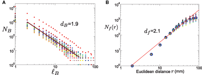
Figure 5. (A) Fractal dimension $d_B$ of the network clusters. The line is representative of the average dimension d_B = 1.9. (B) Fractal dimension d_f of the spatially embedded clusters. The large points represent the number of nodes N_f(r) included within a fixed distance r, averaged over all clusters, while smaller points refer to individual clusters. The fitted line corresponds to the average dimension d_f = 2.1.

The cluster structure can be also probed by its topological features when every node-voxel assumes its assigned location at the brain. Each cluster identified by the box-covering algorithm can be mapped to their anatomical projections, where two voxels are still connected according to their correlation but their distance is now defined by the Euclidean three-dimensional spatial distance r (Figure 5B). This mapping allows the use of the classical fractal dimension in real-space for the study of the structure of these functional clusters in the brain.

The method that we use to calculate the fractal dimension here is an alternative method to the one used in Gallos et al. (2012). There, d_f was calculated by measuring the number of nodes, N_C, in a cluster as a function of the cluster diameter. Here, for every cluster we start from a random point and open a circle of radius r and measure the number of nodes N_f(r) in this circle. The dependence of N_f(r) on r for this cluster gives its fractal dimension, and the process is repeated for all clusters. The scaling of the mass N_f(r) (i.e., number of nodes in the cluster) included in a sphere with Euclidean radius r follows the power-law form of equation (2). The calculation of the individual Euclidean fractal dimensions yields an average of d_f = 2.1 ± 0.1 (Figure 5B), which is similar for all clusters, and which is exactly the same as the one found in Gallos et al. (2012). The network fractal dimension of all clusters was systematically lower than the real-space fractal dimension, which was in the range 2–2.4.

It is possible that the difference between the fractal dimensions of individual clusters can be due to systematic variations, influenced by various factors. We performed a number of tests to identify the stability of these calculations. In Figure 6A we show a cross-plot for the exponents d_B and d_f, as calculated for each individual cluster. The value of d_B was systematically below d_f. From the same plot we deduce that the value of the percolation transition does not influence the fractal dimension, since the different p_c values of different clusters yield a uniform spreading of the fractal dimensions. It is also possible that the location of the brain clusters may have an effect on their fractal character. Our results do not provide any evidence toward this direction, either. In Figure 6B we plot the exponents d_B and d_f for each cluster as a function of the y-coordinate of the cluster’s center of mass, i.e., increasing y indexes corresponds to moving from the posterior to the anterior part of the brain. It is obvious that there is no systematic variation of the exponents in different locations. The above results emphasize the robustness of the fractal structure and indicate that we can consider the averages over all those structures to be representative of a typical brain module.

FIGURE 6

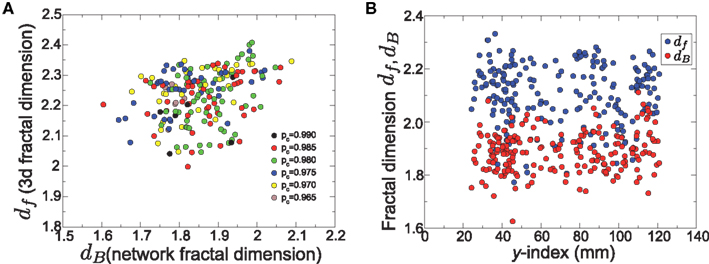
Figure 6. Consistency of the fractal dimension calculations. (A) Cross-plot of d_f vs d_B for individual brain clusters. The colors correspond to the threshold values of p_c where the first percolation transition was identified. (B) The network fractal dimension, d_f (blue), and the three-dimensional fractal dimension, d_B (red) as a function of the location of each cluster. This location corresponds to the center of mass, and is expressed through the y-index, posterior to anterior.

We can now characterize each single cluster, both at the functional level and at the topological level (i.e., the shape that the cluster assumes in the brain). Together, these results indicate that none of the clusters fill the 3D space densely; although the objects are embedded in three-dimensions their fractal dimension d_f is significantly smaller than 3. The network structure provides information on functional clusters, since it relates areas that are highly correlated independently of their physical proximity. Since the network fractal dimension d_B is even smaller than d_f, connections are fewer than one would expect through nearest-neighbor connections only. In simpler words, clusters do not form densely connected neighborhoods.

3.3. Modular Structure

In the Materials and Methods section we described how we can use the optimal MEMB coverage of the network with N_B nodes for a given ℓ_B value, in order to characterize the network modularity. Analysis of the modularity equation (4) in Figure 7 reveals a monotonic increase of ℳ(ℓ_B) with a lack of a characteristic value of ℓ_B. Indeed, the data can be approximately fitted with a power-law functional form, equation (5), which is characterized by the modularity exponent d_M. We analyze the resulting networks of different subjects and we find that d_M = 1.9 ± 0.1 is approximately constant over different individuals (Figure 7).

FIGURE 7

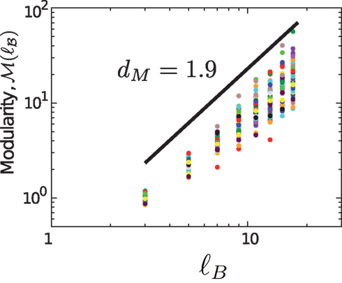
Figure 7. Modularity as a function of ℓ_B for different clusters. The average value of the exponent is d_M = 1.9, shown by the solid line.

This value reveals a considerable degree of modularity in the entire system as evidenced by the network structure. For comparison, a random network has d_M = 0 and a uniform lattice has d_M = 1 (Gallos et al., 2007). The lack of a characteristic length-scale in the modularity shown in Figure 7 suggests that the modules appear at all length-scales, i.e., modules are organized within larger modules in a self-similar way, so that the inter-connections between those clusters repeat the basic modular character of the entire brain network. Thus, the modular organization of the network remains statistically invariant when observed at different scales.

3.4. Short-Cut Wiring is Optimized for Efficient Flow

A major advantage of the present analysis approach is that the analysis of the type of short-cuts present in the brain networks can convey a notion of optimal navigability in the network.

The addition of long-range links can turn the balance of a network structure toward either a self-similar structure with significant modularity but poor transfer or toward a small-world structure with very efficient flow at the cost of modularity (specialization). A small number of such short-cuts, quantified through renormalization group analysis (Rozenfeld et al., 2010), has been shown to provide the optimal trade-off between these two properties. In the case of the brain clusters the need for specialization/modularity is obvious, as also shown in the previous section, so it is important to understand how short-cuts influence the efficiency of signal transport in these structures.

In order to study how the modules that we recovered by the first percolation transition integrate at a larger scale, we also considered another percolation transition that corresponds to the emergence of a spanning cluster. We chose this transition as the correlation point where the largest cluster is equal to half of the total size. This global network connects practically all the smaller brain modules.

We probed the connectivity for this network, by analyzing the distance distribution of the links in the network, i.e., the Euclidean distance between any two voxels that are connected through their phase correlation (Figure 8A). We find an approximately power-law distribution (Figure 8B) of the form:

$P\left(r\right)\sim r^{-\alpha },$(6)

with a short-cut exponent α ≈ 3.1. The value of this exponent is very significant, since it approximately satisfies the scaling relation with the fractal dimension of the brain network:

$\alpha =d_f+1.$(7)

Such a scaling relation was recently (Li et al., 2010) found to optimize the transfer of information across a network with fractal dimension d_f when the short-cuts in the network are added with a cost constraining the number of total links. Thus, our scaling and modular analysis suggests that, taking into account the spatial restrictions, the functional behavior of the brain is optimally wired for facilitating efficient information transfer among different areas.

FIGURE 8

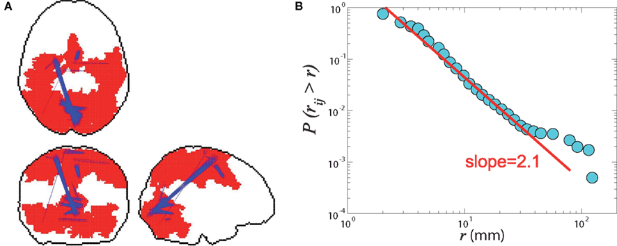
Figure 8. (A) Real-space representation of the network at the second global percolation. The largest component is half the total mass. The blue lines highlight the longest links in Euclidean distance, which correspond to the weak ties. (B) Cumulative probability distribution P(r_ij > r) of Euclidean distances r_ij between any two voxels that are directly connected in the correlation network. The straight line fitting yields an exponent α − 1 = 2.1 ± 0.1 indicating optimal information transfer with wiring cost minimization.

4. Discussion

Our analysis revealed a fractal structure for the individual brain clusters. These clusters have a consistent topological behavior and are located at the areas that correspond to the expected brain responses. These modular structures present consistent fractal properties, both at the functional level and at a topological level. This indicates that the individual processing units that we recover do not have significant small-world properties. In contrast, when we include weaker correlations, the modules that appear at smaller scales are connected through long-range links. These short-cuts give a small-world character to the brain network as a whole, i.e., when studied at scales larger than an individual module.

The study of the distribution for these links suggests interestingly that they are optimizing transfer network properties, by also considering the wiring cost. In simpler terms, this topology does not minimize the global connectivity, simply to connect all the nodes; instead it minimizes the amount of wire required to achieve the goal of shrinking the network to a small-world.

The existence of modular organization of strong ties in a sea of weak ties is reminiscent of the structure found to bind dissimilar communities in social networks. Granovetter’s (1973) work in social sciences proposes the existence of weak ties to cohese well-defined social groups into a large-scale social network. Such a two-scale structure has a large impact on the diffusion and influence of information across the entire social structure. Our observation of this two-layer organization in brain networks suggests that it may be a ubiquitous natural solution to the puzzle of information flow in highly modular structures.

Previous studies have found that wiring of neuronal networks at the cellular level is close to optimal (Song et al., 2005b). Specifically it is found that long-range connections do not minimize wiring but achieve network benefits. In agreement with this observation, at the mesoscopic scale explored here, we find an optimization which reduces wiring cost while maintaining network proximity. An intriguing element of our observation is that this minimization assumes that broadcasting and routing information are known to each node. How this may be achieved – what aspects of the neural code convey its own routing information – remains an open question in Neuroscience.

Conflict of Interest Statement

The authors declare that the research was conducted in the absence of any commercial or financial relationships that could be construed as a potential conflict of interest.

Acknowledgments

We thank D. Bansal, S. Dehaene, S. Havlin, and H. D. Rozenfeld for valuable discussions. Lazaros K. Gallos and Hernán A. Makse thank the NSF-0827508 Emerging Frontiers Program for financial support. Mariano Sigman is supported by a Human Frontiers Science Program Fellowship.

References

Bullmore, E., and Sporns, O. (2009). Complex brain networks: graph theoretical analysis of structural and functional systems. Nat. Rev. Neurosci. 10, 186.

Pubmed Abstract | Pubmed Full Text | CrossRef Full Text

Bunde, A., and Havlin, S. (1996). "Percolation I," in Fractals and Disordered Systems, 2nd Edn, eds A. Bunde, and S. Havlin (Heidelberg: Springer-Verlag), 51–96.

Caldarelli, G., and Vespignani, A. (eds). (2007). Large Scale Structure and Dynamics of Complex Networks. Singapore: World Scientific.

Dux, P. E., Ivanoff, J., Asplund, C. L., and Marois, R. (2006). Isolation of a central bottleneck of information processing with time-resolved fMRI. Neuron 52, 1109.

Pubmed Abstract | Pubmed Full Text | CrossRef Full Text

Eguiluz, V. M., Chialvo, D. R., Cecchi, G. A., Baliki, M., and Apkarian, A. V. (2005). Scale-free brain functional networks. Phys. Rev. Lett. 94, 018102.

Pubmed Abstract | Pubmed Full Text | CrossRef Full Text

Gallos, L. K., Makse, H. A., and Sigman, M. (2012). A small-world of weak ties provides optimal global integration of self-similar modules in functional brain networks. Proc. Natl. Acad. Sci. U.S.A. 109, 2825.

Pubmed Abstract | Pubmed Full Text | CrossRef Full Text

Gallos, L. K., Song, C., Havlin, S., and Makse, H. A. (2007). Scaling theory of transport in complex biological networks. Proc. Natl. Acad. Sci. U.S.A. 104, 7746.

Pubmed Abstract | Pubmed Full Text | CrossRef Full Text

Galvao, V., Miranda, J. G. V., Andrade, R. F. S., Andrade, J. S. Jr., Gallos, L. K., and Makse, H. A. (2010). Modularity map of the network of human cell differentiation. Proc. Natl. Acad. Sci. U.S.A. 107, 5750.

Pubmed Abstract | Pubmed Full Text | CrossRef Full Text

Goh, K. I., Salvi, G., Kahng, B., and Kim, D. (2006). Skeleton and fractal scaling in complex networks. Phys. Rev. Lett. 96, 018701.

Pubmed Abstract | Pubmed Full Text | CrossRef Full Text

Granovetter, M. S. (1973). The strength of weak ties. Am. J. Sociol. 78, 1360.

CrossRef Full Text

Guimerà, R., and Amaral, L. A. N. (2005). Functional cartography of complex metabolic networks. Nature 433, 895.

Pubmed Abstract | Pubmed Full Text | CrossRef Full Text

Kim, J. S., Goh, K. I., Salvi, G., Oh, E., Kahng, B., and Kim, D. (2007). Fractality in complex networks: critical and supercritical skeletons. Phys. Rev. E 75, 016110.

CrossRef Full Text

Li, G. S., Reis, D. S., Moreira, A. A., Havlin, S., Stanley, H. E., and Andrade, J. S. Jr. (2010). Towards design principles for optimal transport networks. Phys. Rev. Lett. 104, 018701.

Pubmed Abstract | Pubmed Full Text | CrossRef Full Text

Menon, R. S., Luknowsky, D. C., and Gati, J. S. (1998). Mental chronometry using latency-resolved functional MRI. Proc. Natl. Acad. Sci. U.S.A. 95, 10902.

Pubmed Abstract | Pubmed Full Text | CrossRef Full Text

Newman, M. E. J., and Girvan, M. (2004). Finding and evaluating community structure in networks. Phys. Rev. E 69, 026113.

CrossRef Full Text

Radicchi, F., Ramasco, J. J., Barrat, A., and Fortunato, S. (2008). Complex networks renormalization: flows and fixed points. Phys. Rev. Lett. 101, 148701.

Pubmed Abstract | Pubmed Full Text | CrossRef Full Text

Rozenfeld, H. D., Song, C., and Makse, H. A. (2010). Small-world to fractal transition in complex networks: a renormalization group approach. Phys. Rev. Lett. 104, 025701.

Pubmed Abstract | Pubmed Full Text | CrossRef Full Text

Sigman, M., and Dehaene, S. (2008). Brain mechanisms of serial and parallel processing during dual-task performance. J. Neurosci. 28, 7585.

Pubmed Abstract | Pubmed Full Text | CrossRef Full Text

Sigman, M., Jobert, A., and Dehaene, S. (2007). Parsing a sequence of brain activations of psychological times using fMRI. Neuroimage 35, 655.

Pubmed Abstract | Pubmed Full Text | CrossRef Full Text

Song, C., Gallos, L. K., Havlin, S., and Makse, H. A. (2007). How to calculate the fractal dimension of a complex network: the box covering algorithm. J. Stat. Mech. 2007, P03006.

CrossRef Full Text

Song, C., Havlin, S., and Makse, H. A. (2005a). Self-similarity of complex networks. Nature 433, 392.

CrossRef Full Text

Song, S., Sjostrom, P. J., Reigl, M., Nelson, S., and Chklovskii, D. B. (2005b). Highly nonrandom features of synaptic connectivity in local cortical circuits. PLoS Biol. 3, e68.

CrossRef Full Text

Song, C., Havlin, S., and Makse, H. A. (2006). Origins of fractality in the growth of complex networks. Nat. Phys. 2, 275.

CrossRef Full Text

Sporns, O., Tononi, G., and Kotter, R. (2005). The human connectome: a structural description of the human brain. PLoS Comput. Biol. 1, e42.

CrossRef Full Text

Stanley, H. E. (1971). Introduction to Phase Transitions and Critical Phenomena. Oxford: Oxford University Press.

Vicsek, T. (1992). Fractal Growth Phenomena, 2nd Edn, Part IV. Singapore: World Scientific.

Watts, D., and Strogatz, S. (1998). Collective dynamics of “small-world” networks. Nature 393, 440.

Pubmed Abstract | Pubmed Full Text | CrossRef Full Text