An Analytical Framework for Studying Small-Number Effects in Catalytic Reaction Networks: A Probability Generating Function Approach to Chemical Master Equations

Cell activities primarily depend on chemical reactions, especially those mediated by enzymes, and this has led to these activities being modeled as catalytic reaction networks. Although deterministic ordinary differential equations of concentrations (rate equations) have been widely used for modeling purposes in the field of systems biology, it has been pointed out that these catalytic reaction networks may behave in a way that is qualitatively different from such deterministic representation when the number of molecules for certain chemical species in the system is small. Apart from this, representing these phenomena by simple binary (on/off) systems that omit the quantities would also not be feasible. As recent experiments have revealed the existence of rare chemical species in cells, the importance of being able to model potential small-number phenomena is being recognized. However, most preceding studies were based on numerical simulations, and theoretical frameworks to analyze these phenomena have not been sufficiently developed. Motivated by the small-number issue, this work aimed to develop an analytical framework for the chemical master equation describing the distributional behavior of catalytic reaction networks. For simplicity, we considered networks consisting of two-body catalytic reactions. We used the probability generating function method to obtain the steady-state solutions of the chemical master equation without specifying the parameters. We obtained the time evolution equations of the first- and second-order moments of concentrations, and the steady-state analytical solution of the chemical master equation under certain conditions. These results led to the rank conservation law, the connecting state to the winner-takes-all state, and analysis of 2-molecules M-species systems. A possible interpretation of the theoretical conclusion for actual biochemical pathways is also discussed.

1. Introduction

Biochemical systems consist of a variety of chemicals, including proteins, nucleic acids, and also small metabolites. Enzymatic reactions, which play an important role in catalyzing many biological reactions, are particularly important to maintain the structure and activity of these systems. Hence, biochemical systems are often modeled as catalytic reaction networks.

These networks are typically analyzed by using deterministic ordinary differential equations with respect to concentrations of chemical species, so-called reaction rate equations [or partial differential equations (reaction-diffusion equations) for spatially distributed, non-uniform cases]; i.e., the concentrations are represented by continuous variables. However, because each chemical actually consists of molecules, the concentration of each species should be a discrete variable. The effects of such discreteness as well as finite-size fluctuations in stochastic reactions become non-negligible if the number of molecules in the system is small. In theory, situations such as these can result in phenomena that cannot be described by rate equations (as well as those equations with additional noise; Togashi and Kaneko, 2001, 2007; Awazu and Kaneko, 2007, 2009).

In contrast, gene regulations are often modeled as a combination of binary (on/off) switches, typically represented by Boolean network models (Kauffman, 1969). However, this approach does not consider the quantities of chemicals such as DNA, mRNA, and proteins. Even for the seemingly digital expression of genes, a stoichiometry involving DNA cannot be ignored, as seen in X-chromosome inactivation (2 to 1) and the trisomy syndrome (2 to 3). Thus, the use of a binary (on/off) representation would also be inappropriate. We therefore need to consider the number of molecules.

Recent experiments have shown the existence in the cell of proteins that only consist of a few molecules each (Taniguchi et al., 2010), and these potential biological phenomena (sometimes referred to as the small-number issue) have been gradually recognized by biologists. General theories that would enable predictions in small number situations would be helpful to every biological scientist seeking to understand biochemical processes on any level. Of course, the distributional behavior of such discrete stochastic systems is described by the chemical master equation. However, it is generally difficult to obtain its solution; hence, most efforts have been devoted to the development of approximation and simulation methods and their application (Gillespie, 1976, 1977; Munsky and Khammash, 2006; Lee et al., 2009; Kim and Lee, 2012).

The effects of small numbers in particular systems, e.g., small autocatalytic systems have been mathematically analyzed (Ohkubo et al., 2008; Biancalani et al., 2012, 2014; Houchmandzadeh and Vallade, 2015; Saito and Kaneko, 2015). In addition, a parameter representing the degree of discreteness in the number of molecules has been introduced (Haruna, 2010, 2015). In this work, we pursue analytical frameworks for studying the effects of small numbers in catalytic reaction networks by following an approach that is as general as possible. Our aim is to obtain the steady-state analytical solution for the chemical master equation without specifying parameters, rather than developing numerical schemes to solve it as was previously done (Kim and Lee, 2012). Furthermore, we try to theoretically describe the long-term behavior of the system by only using information about relationships between elements, thereby implying that we aim to produce results that could be applied to studies in any field.

Our framework provides good operability because our formulas have a specific and satisfyingly simple form, and enables us to obtain the steady state for a wide class of catalytic reaction networks because our framework never specifies any parameters for the networks. We use a probability generating function approach. The probability generating function approach to stochastic chemical kinetics itself has been proposed a long time ago (e.g., Krieger and Gans, 1960; McQuarrie, 1967), after which it spread to biological stochastic kinetics studies (e.g., stochastic gene expression Thattai and van Oudenaarden, 2001; Shahrezaei and Swain, 2008); thus, physicists as well as chemists and mathematical biologists are familiar with the approach. Our main contributions in this paper relate to the efficient usage of the probability generating function (as in Gadgil et al., 2005 regarding first-order reaction networks). Therefore, our approach for obtaining the steady state is understandably easier than that followed in a previous study (Anderson et al., 2010) while, as a consequence, our results are consistent with that study (see Theorem 4.1 and 4.2 in Anderson et al., 2010). Furthermore, since our method uses a procedure based on analytical calculations, it can be easily converted to a computer algorithm.

The present paper is organized as follows. In Section 2.1, we define the catalytic reaction network considered in this paper. The chemical master equation (CME) is provided in Section 2.2. We introduce the probability generating function (PGF) and derive the generating function equation (GFE) in Section 2.3. In subsequent Sections (2.3.1–2.3.3), we show that the GFE introduces the time evolution equation of the first-order and second-order moments of concentrations (we refer to the first-order moment time evolution equation as the pre-rate equation, PRE), and the second-order moment expression of time-averaged concentrations (SME). Section 2.4 is devoted to obtaining the steady-state solutions of the GFE. To simplify the GFE, we neglect the non-catalytic reactions considered as perturbation for the catalytic reaction network if the system is “entirely ergodic.” In Section 2.4.2.3 as the main result, we obtain the probability generating function without winner-takes-all states (PGFwoWTAS) including the solutions of the corresponding rate equation. In Section 3, we describe applications of these results: the rank conservation law, the connecting state to the winner-takes-all state, analysis of 2-molecules M-species systems, and non-autocatalyzation of autocatalytic reaction networks. The prospects of our theory in terms of the small-number issue are briefly discussed in Section 4.

2. Methods and Results

2.1. Catalytic Reaction Networks

Consider an abstract catalytic reaction network consisting of M chemical species and N molecules in a well-stirred reactor of volume V, as in Awazu and Kaneko (2007). Each species is labeled by each of the integers between 1 and M. The total number of molecules N is always conserved in reaction processes. This chemical reaction system involves both catalytic reactions and non-catalytic reactions, to prevent catalytic reactions from stopping:

(i) Catalytic reactions (two-body catalysis):

$\begin{array}{lll}i\stackrel{j}{\to }k,\hfill & & (1)\end{array}$

where the species i, j, k ∈ [1, M] represent a substrate, a catalyst, and a product. The reaction rate constant is represented by R_ijk > 0. If this catalytic reaction does not exist, we specify R_ijk = 0. Therefore, the catalytic reaction networks are determined by R_ijk. In this paper, we impose the following conditions for the catalytic reaction networks;

(a) R_iik = 0; Substrate ≠ Catalyst.

(b) R_iji = 0; Substrate ≠ Product.

(c) R_ikk = 0; Autocatalytic reactions are not included.

(d) #{k : R_ijk > 0 (∀i, j)} = 1;

One product against a substrate and a catalyst.

(ii) Non-catalytic reactions (one-body reactions):

$\begin{array}{ll}i\stackrel{\text{Prob.\hspace{0.05em}}1/M}{\to }j.\hfill & (2)\end{array}$

This reaction exists for all combinations between each species, but a product j ∈ [1, M] is uniformly-randomly selected from all species 1 to M. The rate constant is set ε > 0 in common, where ε is very small, i.e., ε ≪ min{R_ijk > 0}.

The state of this catalytic reaction network is specified by the combination of M natural numbers n = (n₁, n₂, ⋯ , n_M), where n_i ∈ [0, N] is the number of molecules of the ith-species. For later convenience, we introduce the following notations: the state space of the catalytic reaction network W_{M, N} (abbr. W) is represented by

$\begin{array}{lll}W:=\left\{\mathbf{n}\in {\left[0,N\right]}^M\mid n_1+\cdots +n_M=N\right\},\hfill & & (3)\end{array}$

which consists of $\left((\frac{M}{N})\right):=\frac{(N+M-1)!}{(M-1)!N!}$ points; a collection consisting of (one species) winner-takes-all states I_{M, N} (abbr. I) is represented by

$\begin{array}{lll}I:=\left\{\mathbf{n}\in W_{M,N}\mid \exists i\in \left[1,M\right]\text{ s.t.}{n}_i=N\right\},\hfill & & (4)\end{array}$

which consists of M points. Of course, the winners-take-all states of more than one species can be considered, but we focus on the winner-takes-all states of one species by supposing the system satisfies a certain condition, entire ergodicity (see Section 2.4.2.4).

In the present paper, we are interested in the N-dependence of the concentration of each species x_i = n_i/V. We basically consider a situation in which the total density of molecules ρ = N/V is conserved, even if the total number of molecules N is changed.

2.2. The Chemical Master Equation

The rate constant R_ijk in the catalytic reaction is defined as the number of reactions per unit volume, unit concentration, and unit time. Therefore, the number of reactions per unit time in the catalytic reaction $i\stackrel{j}{\to }k$, such that the concentrations are x_i and x_j, is

$\begin{array}{lll}{R}_{ijk}{x}_i{x}_{j}V=R_{ijk}\frac{n_i{n}_j}{V}=R_{ijk}\frac{n_i{n}_j}{N}\rho ,\hfill & & (5)\end{array}$

where ρ = N/V is the total density of molecules in the vessel. On the other hand, the number of reactions per unit time in the non-catalytic reaction i → j with probability 1/M is

$\begin{array}{lll}\epsilon x_{i}V\times \frac{1}{M}=\frac{\epsilon }{M}{n}_i.\hfill & & (6)\end{array}$

Then, the time-evolution of the probability P(n, t), with which the system is in the state n at time t, obeys the chemical master equation (CME):

$\begin{array}{l}\frac{dP(\mathbf{n},t)}{dt}=\frac{\rho }{N}{\displaystyle \sum _{i,j,k}}{R}_{ijk}(E_i^{+1}{E}_k^{-1}-1)n_i{n}_{j}P(\mathbf{n},t)\\ +\frac{\epsilon }{M}{\displaystyle \sum _{i,j}}(E_i^{+1}{E}_j^{-1}-1)n_{i}P(\mathbf{n},t),& (7)\end{array}$

where $E_i^{\pm m}$ are step operators, i.e.,

$\begin{array}{lll}{E}_i^{\pm m}f(n_1,\cdots ,n_i,\cdots ,n_M):=f(n_1,\cdots ,n_i\pm m,\cdots ,n_M).\hfill & & (8)\end{array}$

Of course, the state space on which the probability P(·, t) is supported, is the previously described W_{M, N}.

2.3. Probability Generating Function Method

The probability generating function (PGF) is useful to analyze the CME:

$\begin{array}{ll}\varphi (\mathbf{z},t):={\displaystyle \sum _{n_1,\cdots ,n_M}P}(\mathbf{n},t)z_1{}^{n_1}\cdots z_M{}^{n_M}.\hfill & (9)\end{array}$

Note that the following expressions are translated to differential forms of the PGF:

$\begin{array}{lll}{n}_{i}P(\mathbf{n},t)\hfill & \mapsto z_i\frac{\partial }{\partial z_i}\varphi (\mathbf{z},t),& (\mathrm{10a})\end{array}$

$\begin{array}{lll}{n}_i{n}_{j}P(\mathbf{n},t)\hfill & \mapsto z_i{z}_j\frac{\partial }{\partial z_i}\frac{\partial }{\partial z_j}\varphi (\mathbf{z},t)(i\ne j),& (\mathrm{10b})\end{array}$

$\begin{array}{lll}{E}_i^{+1}{E}_j^{-1}{n}_{i}P(\mathbf{n},t)\hfill & \mapsto z_j\frac{\partial }{\partial z_i}\varphi (\mathbf{z},t)(i\ne j),& (\mathrm{10c})\end{array}$

$\begin{array}{lll}{E}_i^{+1}{E}_k^{-1}{n}_i{n}_{j}P(\mathbf{n},t)\hfill & \mapsto z_j{z}_k\frac{\partial }{\partial z_i}\frac{\partial }{\partial z_j}\varphi (\mathbf{z},t)(i\ne j\ne k\ne i).& (\mathrm{10d})\end{array}$

Therefore, rewriting the CME to the equation governing the PGF enables the generating function equation (GFE) to be obtained:

$\begin{array}{l}\frac{\partial \varphi (\mathbf{z},t)}{\partial t}=\frac{\rho }{N}{\displaystyle \sum _{i,j,k}}{R}_{ijk}(z_k-z_i)z_j\frac{\partial }{\partial z_i}\frac{\partial }{\partial z_j}\varphi (\mathbf{z},t)\\ +\frac{\epsilon }{M}{\displaystyle \sum _{i,j}}(z_i-z_j)\frac{\partial }{\partial z_j}\varphi (\mathbf{z},t).& (11)\end{array}$

The GFE consists of continuous variables, unlike the CME, which consists of discrete variables.

Once we obtain the PGF ϕ as a solution to the GFE, we can derive all statistics of the catalytic reaction network; for example, the ensemble averages (first-order moments) and second-order moments become

$\begin{array}{ll}\langle n_i\rangle (t)={\frac{\partial }{\partial z_i}\varphi (\mathbf{z},t)|}_{\mathbf{z}=\mathbf{1}},\hfill & (\mathrm{12a})\end{array}$

$\begin{array}{ll}\langle n_i{n}_j\rangle (t)={\frac{{\partial }^2}{\partial z_i\partial z_j}\varphi (\mathbf{z},t)|}_{\mathbf{z}=\mathbf{1}}(i\ne j),\hfill & (\mathrm{12b})\end{array}$

$\begin{array}{ll}\langle n_l(n_l-1)\rangle (t)={\frac{{\partial }^2}{\partial z_l^2}\varphi (\mathbf{z},t)|}_{\mathbf{z}=\mathbf{1}},\hfill & (\mathrm{12c})\end{array}$

and the marginal distributions become

$\begin{array}{ll}{p}_i(n,t)=\frac{1}{n!}{\frac{{\partial }^n}{\partial z_i^n}\varphi (\mathbf{z},t)|}_{z_i=0;z_j=1(j\ne i)}(0\le n\le N),\hfill & (13)\end{array}$

where p_i(n, t) is defined by

$\begin{array}{ll}{p}_i(n,t):={\displaystyle \sum _{\begin{array}{c}{n}_1,\cdots ,n_M\\ (\text{except\hspace{0.17em}}{n}_i)\end{array}}{P(\mathbf{n},t)|}_{n_i=n}}.\hfill & (14)\end{array}$

2.3.1. The Pre-rate Equation

Rate equations are differential equations for the concentrations x_i of chemical species i = 1, ⋯ , M when N → ∞. We use the GFE to derive a formula, which is reminiscent of the rate equation.

Differentiating both sides of Equation (11) by z_i, substituting z = 1, and writing x_i = n_i/V, leads to the following pre-rate equation (PRE);

$\begin{array}{ll}\frac{d}{dt}\langle x_i\rangle ={\displaystyle \sum _{j,k}}\left(R_{jki}\langle x_j{x}_k\rangle -R_{ikj}\langle x_i{x}_k\rangle \right)+\epsilon \left(\frac{\rho }{M}-\langle x_i\rangle \right).\hfill & (15)\end{array}$

Note that, as we are considering a system of which the total number of molecules N is conserved, the concentration conservation law (CCL) must be satisfied;

$\begin{array}{ll}{\displaystyle \sum _i}\langle x_i\rangle (t)=\rho (\forall t),\hfill & (16)\end{array}$

where the PRE (Equation 15) is consistent with the CCL (Equation 16).

If the independence 〈x_ix_j〉 = 〈x_i〉〈x_j〉 (i ≠ j) holds, the PRE (Equation 15) becomes the same expression as the rate equation. On the other hand, the PRE does not explicitly include extensive variables, such as the total number of molecules N. Therefore, the formula (Equation 15) always holds for an arbitrary molecular number N unless the total molecular density ρ is changed.

2.3.2. Second-Order Moment Expression for Time-Averaged Concentrations

We suppose the following ergodicity to replace ensemble-averages with time-averages; ${\overline{n}}_i={\langle n_i\rangle }_{*}$ i.e.,

$\begin{array}{ll}{\displaystyle \underset{T\to \infty }{lim}}\frac{1}{T}{\displaystyle {\int }_0^T}{n}_i(t)dt={\displaystyle \sum _{n_1,\cdots ,n_M}}{n}_i{P}_{*}(\mathbf{n}),\hfill & (17)\end{array}$

where P_*(n) is the steady-state solution of the CME corresponding to almost all initial conditions. Considering the steady state in the PRE [that is, taking t → ∞ on both sides of Equation (15)], one obtains the following second-order moment expression (SME) for time-averaged concentrations:

$\begin{array}{ll}{\overline{x}}_i=\frac{\rho }{M}+\frac{1}{\epsilon }{\displaystyle \sum _{j,k}}\left(R_{jki}\overline{x_j{x}_k}-R_{ikj}\overline{x_i{x}_k}\right).\hfill & (18)\end{array}$

The second term on the right hand side of Equation (18) represents the difference from the uniform concentration ρ/M.

If the independence $\overline{x_i{x}_j}={\overline{x}}_i{\overline{x}}_j$ holds, Equation (18) becomes an equation that only includes the concentrations ${\overline{x}}_i$. Therefore, in combination with the time-averaged version of the CCL (Equation 16), the concentrations ${\overline{x}}_i$ can be determined without including unknown quantities. However, the actual concentrations ${\overline{x}}_i$ depend on their second-order moments $\overline{x_i{x}_j}$.

2.3.3. Time-Evolution of Second-Order Moments

Determining the concentrations ${\overline{x}}_i$ from the SME (Equation 18) requires us to know their second-order moments $\overline{x_i{x}_j}$.

Differentiating both sides of the GFE (Equation 11) by z_l and z_m (l ≠ m), substituting z = 1, and writing x_i = n_i/V, then, after simplification, the following time-evolution equation of second-order moments (TESM) is obtained:

$\begin{array}{l}\frac{d}{dt}\langle x_l{x}_m\rangle =-\frac{\rho }{N}{\displaystyle \sum _i(R_{lim}\langle }{x}_i{x}_l\rangle +R_{mil}\langle x_i{x}_m\rangle )\\ +{\displaystyle \sum _{i,j}\{R_{ijl}\langle }{x}_i{x}_j{x}_m\rangle +R_{ijm}\langle x_i{x}_j{x}_l\rangle -(R_{lij}+R_{mij})\\ \langle x_i{x}_l{x}_m\rangle \}\\ +\frac{\epsilon }{M}\left\{\frac{N-1}{N}\rho (\langle x_l\rangle +\langle x_m\rangle )-2M\langle x_l{x}_m\rangle \right\}\\ (1\le l<m\le M).& (\mathrm{19a})\end{array}$

On the other hand, twice differentiating both sides of the GFE (Equation 11) by z_l, substituting z = 1, and writing x_i = n_i/V, then after some simplification, the following alternative TESM is obtained:

$\begin{array}{l}\frac{d}{dt}\langle x_l(x_l-\frac{\rho }{N})\rangle =2{\displaystyle \sum _{i,j}}\left(R_{ijl}\langle x_i{x}_j{x}_l\rangle -R_{lij}\langle x_i{x}_l(x_l-\frac{\rho }{N})\rangle \right)\hfill \\ +\frac{2\epsilon }{M}\left\{\frac{N+M-1}{N}\rho \langle x_l\rangle -M\langle x_l^2\rangle \right\}\hfill \\ (1\le l\le M).\hfill & (\mathrm{19b})\end{array}$

The expression of TESMs (Equation 19) consists of M(M+1)/2 equations containing the third-order moments 〈x_ix_jx_k〉(t). Therefore, the TESMs are not effective unless the systems are restricted such that the third-order moments vanish (e.g., 2-molecules systems). If N = 2, because ${\partial }_{z_i}$${\partial }_{z_j}$${\partial }_{z_k}$ϕ = 0 (ϕ is a second-order polynomial), one can calculate the 2-molecules version of the TESMs (2mTESMs);

$\begin{array}{l}\frac{d}{dt}\langle x_l{x}_m\rangle =\frac{\rho }{2}{\displaystyle \sum _i\{R_{iml}\langle }{x}_i{x}_m\rangle +R_{ilm}\langle x_i{x}_l\rangle \\ -(R_{lmi}+R_{mli})\langle x_l{x}_m\rangle \}\\ +\frac{\rho \epsilon }{2M}(\langle x_l\rangle +\langle x_m\rangle )-2\epsilon \langle x_l{x}_m\rangle \\ (1\le l<m\le M),& (\mathrm{20a})\end{array}$

$\begin{array}{ll}\frac{d}{dt}\langle x_l(x_l-\frac{\rho }{N})\rangle =\frac{2\epsilon }{M}\left(\frac{M+1}{2}\rho \langle x_l\rangle -M\langle x_l^2\rangle \right)(1\le l\le M).\hfill & (\mathrm{20b})\end{array}$

Treatment of the 2mTESMs (Equation 20) to demonstrate their effectiveness appears in a later section.

2.4. Steady-State Solutions of GFE

If the GFE (Equation 11) can be solved, this would enable us to obtain all the statistics of the catalytic reaction networks. However, it is generally difficult to solve. Here, we focus on the steady-state solutions of the GFE and consider the case that the ε-term in the GFE can be ignored. Through the following discussion, we see that the approximation is effective only if the system is ergodic.

2.4.1. The Case of Non-catalytic Reactions Only

First, we consider the steady-state solutions of non-catalytic reactions only as an introduction. The PGF ${\varphi }_{*}^{\mathrm{\text{nc}}}(\mathbf{z})$, corresponding to the steady state in the case of non-catalytic reactions only, should satisfy the following equation:

$\begin{array}{ll}0={\displaystyle \sum _{i,j}}(z_i-z_j)\frac{\partial }{\partial z_j}{\varphi }_{*}^{\mathrm{\text{nc}}}(\mathbf{z}).\hfill & (21)\end{array}$

By exchanging the subscripts i and j in the second term, one obtains

$\begin{array}{ll}0={\displaystyle \sum _{i,j}}{z}_i\left(\frac{\partial {\varphi }_{*}^{\mathrm{\text{nc}}}}{\partial z_j}-\frac{\partial {\varphi }_{*}^{\mathrm{\text{nc}}}}{\partial z_i}\right).\hfill & (22)\end{array}$

Because the coefficients of variables z_i must be zero, ${\varphi }_{*}^{\mathrm{\text{nc}}}$ must satisfy the following equations:

$\begin{array}{ll}0={\displaystyle \sum _j}\left(\frac{\partial {\varphi }_{*}^{\mathrm{\text{nc}}}}{\partial z_j}-\frac{\partial {\varphi }_{*}^{\mathrm{\text{nc}}}}{\partial z_i}\right)(\forall i),\hfill & (23)\end{array}$

equivalently,

$\begin{array}{ll}\frac{\partial {\varphi }_{*}^{\mathrm{\text{nc}}}}{\partial z_i}=\frac{1}{M}{\displaystyle \sum _{j=1}^M}\frac{\partial {\varphi }_{*}^{\mathrm{\text{nc}}}}{\partial z_j}(\forall i).\hfill & (24)\end{array}$

Equation (24) implies that all of ${\partial }_{z_i}{\varphi }_{*}^{\mathrm{\text{nc}}}$ (i = 1, ⋯ , M) are equal to each other, i.e.,

$\begin{array}{ll}\frac{\partial {\varphi }_{*}^{\mathrm{\text{nc}}}}{\partial z_i}=\frac{\partial {\varphi }_{*}^{\mathrm{\text{nc}}}}{\partial z_j}(1\le i<j\le M).\hfill & (25)\end{array}$

Considering that the PGF ${\varphi }_{*}^{\mathrm{\text{nc}}}(\mathbf{z})$ is an Nth order polynomial of z_i and must satisfy the condition ${\varphi }_{*}^{\mathrm{\text{nc}}}(1)=1$ by definition, the following solution of Equation (25) can be found:

$\begin{array}{ll}{\varphi }_{*}^{\mathrm{\text{nc}}}(\mathbf{z})={\left(\frac{z_1+z_2+\cdots +z_M}{M}\right)}^N.\hfill & (26)\end{array}$

Therefore, we obtain the following stationary distribution in the case of non-catalytic reactions only:

$\begin{array}{ll}{P}_{*}^{\mathrm{\text{nc}}}(\mathbf{n})=\frac{1}{M^N}\left(\genfrac{}{}{0.0pt}{}{N}{n_1,n_2,\cdots ,n_M}\right)(\mathbf{n}\in W),\hfill & (27)\end{array}$

where $\left(\genfrac{}{}{0.0pt}{}{N}{n_1,n_2,\cdots ,n_M}\right):=\frac{N!}{n_1!n_2!\cdots n_M!}$ are multinomial coefficients. Furthermore, Equation (13) can also be used to derive the marginal distribution of the i-th species:

$\begin{array}{ll}{p}_{i*}^{\mathrm{\text{nc}}}(\mathbf{n})=\left(\genfrac{}{}{0.0pt}{}{N}{n}\right){\left(\frac{1}{M}\right)}^n{\left(1-\frac{1}{M}\right)}^{N-n}(0\le n\le N),\hfill & (28)\end{array}$

which is the binomial distribution with parameters N and 1/M.

If we suppose the ergodicity $\langle n_i\rangle ={\overline{n}}_i$, the following statistics can be calculated from Equation (12):

$\begin{array}{ll}{\overline{x}}_i=\frac{\rho }{M}(i=1,\cdots ,M),\hfill & (\mathrm{29a})\end{array}$

$\begin{array}{ll}\overline{x_i{x}_j}={\left(\frac{\rho }{M}\right)}^2\left(1-\frac{1}{N}\right)(i\ne j),\hfill & (\mathrm{29b})\end{array}$

$\begin{array}{ll}\mathrm{Var}\left[x_i\right]={\left(\frac{\rho }{M}\right)}^2\frac{M-1}{N}(i=1,\cdots ,M),\hfill & (\mathrm{29c})\end{array}$

where $\mathrm{Var}\left[x_i\right]:=\overline{x_i^2}-{\overline{x_i}}^2$ is the variance of the concentration x_i = n_i/V.

2.4.2. The Case of Catalytic Reactions Only

Next, we consider the steady-state solutions of catalytic reactions only, assuming that the ε-term in the GFE (Equation 11) can be ignored. The steady-state solutions are assumed to have a form similar to Equation (26), including undetermined coefficients (λ_i) deriving from the network structure (R_ijk).

2.4.2.1. A condition for finding the steady state: λ-condition

The PGF ${\varphi }_{*}^{\mathrm{\text{c}}}(\mathbf{z})$, corresponding to the steady state in the case of catalytic reactions only, should satisfy the following equation;

$\begin{array}{ll}0={\displaystyle \sum _{i,j,k}}{R}_{ijk}(z_k-z_i)z_j\frac{\partial }{\partial z_i}\frac{\partial }{\partial z_j}{\varphi }_{*}^{\mathrm{\text{c}}}(\mathbf{z}).\hfill & (30)\end{array}$

Construction of the steady-state solution requires us to find a particular solution of Equation (30) as bases of linear space consisting of N-th order polynomials. Accordingly, let us assume the following extended form of Equation (26) by introducing parameters ${\left\{{\lambda }_i\right\}}_{i=1}^M$, which eventually correspond to the concentrations (per total density ρ) of each species in the continuous limit N → ∞ as shown in Section 2.4.2.3:

$\begin{array}{ll}{\varphi }_{*}^{\mathrm{\text{c}}}(\mathbf{z})={\left({\lambda }_1{z}_1+{\lambda }_2{z}_2+\cdots +{\lambda }_M{z}_M\right)}^N,\hfill & (31)\end{array}$

where

$\begin{array}{ll}{\displaystyle \sum _{i=1}^M}{\lambda }_i=1(0\le {\lambda }_1,{\lambda }_2\cdots ,{\lambda }_M\le 1),\hfill & (32)\end{array}$

because ϕ_*(1) = 1. Substituting Equation (31) into Equation (31) and setting the coefficients of variables z_iz_j as zero, gives the following condition for {λ_iλ_j}:

$\begin{array}{l}{\displaystyle \sum _{k=1}^M}\left\{R_{kij}{\lambda }_k{\lambda }_i+R_{kji}{\lambda }_k{\lambda }_j-\left(R_{ijk}+R_{jik}\right){\lambda }_i{\lambda }_j\right\}=0\hfill \\ (1\le i<j\le M).\hfill & (33)\end{array}$

The λ-condition (Equation 33) represents M(M − 1)/2 homogeneous equations for λ_iλ_j; therefore, λ_i can be calculated by combining the λ-condition (Equation 33) with Equation (32). The λ-condition has trivial solutions:

$\begin{array}{ll}({\lambda }_1,\cdots ,{\lambda }_i,\cdots ,{\lambda }_M)=(0,\cdots ,0,1,0,\cdots ,0)\exists i\in \left[1,M\right].\hfill & (34)\end{array}$

These solutions represent the states for which the i-th species take all molecules (the winner-takes-all state). On the other hand, there is also a non-trivial solution. In the following paragraph, we treat three-species systems (M = 3) to demonstrate that non-trivial solutions do exist. The following procedures can easily be extended to those for arbitrary M species systems.

2.4.2.2. Demonstration for non-trivial solutions of the λ-condition

The λ-condition (Equation 33) can be rewritten in matrix form; i.e., in the case of M = 3 for example,

$\begin{array}{ll}\left[\begin{array}{ccc}-R_{123}-R_{213}& -R_{312}& R_{321}\\ R_{213}& -R_{132}-R_{312}& R_{231}\\ R_{123}& R_{132}& -R_{231}-R_{321}\end{array}\right]\left[\begin{array}{ll}{\lambda }_1\hfill & {\lambda }_2\hfill \\ {\lambda }_1\hfill & {\lambda }_3\hfill \\ {\lambda }_2\hfill & {\lambda }_3\hfill \end{array}\right]=0\hfill & (35)\end{array}$

The 3 × 3 matrix (A) on the left-hand side can be rewritten in terms of its column vectors:

$\begin{array}{ll}A=\begin{array}{c}[-R_{123}{\mathbf{e}}_1-R_{213}{\mathbf{e}}_2,R_{312}{\mathbf{e}}_2-R_{132}{\mathbf{e}}_3,R_{321}{\mathbf{e}}_1+R_{231}{\mathbf{e}}_3\end{array}],\hfill & (36)\end{array}$

where ${{\mathbf{e}}_1}^T=(1,0,-1)$, ${{\mathbf{e}}_2}^T=(1,-1,0)$, and ${{\mathbf{e}}_3}^T=(0,1,-1)$. According to the determinant property, i.e., det[a, b, c] = −det[b, a, c], one has

$\begin{array}{ll}det(A)=0.\hfill & (37)\end{array}$

Therefore, the non-trivial solution of Equation (35), i.e., the eigenvector corresponding to the eigenvalue 0 of the matrix A, certainly exists and it has the following expression:

$\begin{array}{ll}\left[\begin{array}{c}{\lambda }_1{\lambda }_2\\ {\lambda }_1{\lambda }_3\\ {\lambda }_2{\lambda }_3\end{array}\right]\propto \left[\begin{array}{c}{R}_{312}{R}_{231}+R_{321}{R}_{132}+R_{312}{R}_{321}\\ R_{213}{R}_{321}+R_{231}{R}_{123}+R_{213}{R}_{231}\\ R_{123}{R}_{312}+R_{132}{R}_{213}+R_{123}{R}_{132}\end{array}\right]\equiv \left[\begin{array}{c}{\Lambda }_3\\ {\Lambda }_2\\ {\Lambda }_1\end{array}\right].\hfill & (38)\end{array}$

The proportionality constant (> 0) can be determined by the condition (Equation 32), and thus the desired non-trivial solution of the λ-condition (Equation 33) for M = 3 is obtained:

$\begin{array}{ll}{\lambda }_1=\frac{{\Lambda }_2{\Lambda }_3}{{\Lambda }_1{\Lambda }_2+{\Lambda }_1{\Lambda }_3+{\Lambda }_2{\Lambda }_3},\hfill & (\mathrm{39a})\end{array}$

$\begin{array}{ll}{\lambda }_2=\frac{{\Lambda }_1{\Lambda }_3}{{\Lambda }_1{\Lambda }_2+{\Lambda }_1{\Lambda }_3+{\Lambda }_2{\Lambda }_3},\hfill & (\mathrm{39b})\end{array}$

$\begin{array}{ll}{\lambda }_3=\frac{{\Lambda }_1{\Lambda }_2}{{\Lambda }_1{\Lambda }_2+{\Lambda }_1{\Lambda }_3+{\Lambda }_2{\Lambda }_3}.\hfill & (\mathrm{39c})\end{array}$

Note that it is not guaranteed that the above solution always represents a non-trivial solution of the λ-condition (Equation 33). For example, the case of Λ₁ = 0 (where Λ₂ and Λ₃ are not zero) implies the existence of a trivial solution (λ₁, λ₂, λ₃) = (1, 0, 0). In another example, the case of Λ₁ = Λ₂ = 0 implies that the denominator becomes zero; thus, the expression becomes indefinite.

2.4.2.3. PGF without winner-takes-all states

We are interested in those states in which any species does not take all molecules, because the actual simulations are performed by using the initial states excluding the winner-takes-all states. The PGF without the winner-takes-all states is represented by a linear summation of winner-takes-all states $z_i^N$ and Equation (31) if the λ-condition has a non-trivial solution like Equation (39);

$\begin{array}{ll}{\varphi }_{*}^{\mathrm{\text{c}}}(\mathbf{z})={\displaystyle \sum _{i=1}^M}{b}_i{z}_i^N+b_{M+1}{\left({\displaystyle \sum _{i=1}^M}{\lambda }_i{z}_i\right)}^N,\hfill & (40)\end{array}$

where b₁+⋯+b_M+1 = 1. The take-all exclusion conditions are that the coefficients of $z_i^N$ are zero;

$\begin{array}{ll}{b}_i+b_{M+1}{\lambda }_i^N=0(i=1,2,\cdots ,M).\hfill & (41)\end{array}$

Therefore, we obtain the desired PGF without the winner-takes-all states (PGFwoWTAS);

$\begin{array}{l}{\varphi }_{*}^{\mathrm{\text{c}}}(\mathbf{z})=\frac{{\left({\displaystyle {\sum }_{i=1}^M}{\lambda }_i{z}_i\right)}^N-{\displaystyle {\sum }_{i=1}^M}{\left({\lambda }_i{z}_i\right)}^N}{1-{\displaystyle {\sum }_{i=1}^M}{\lambda }_i^N},\hfill \\ {\displaystyle \sum _{i=1}^M}{\lambda }_i=1,0\le {\lambda }_i<1,\hfill & (42)\end{array}$

which immediately implies the following stationary distribution in the case of catalytic reactions only;

$\begin{array}{ll}{P}_{*}^{\text{c}}(\mathbf{n})=\{\begin{array}{c}\left(\genfrac{}{}{0.0pt}{}{N}{n_1,n_2,\cdots ,n_M}\right)\frac{{{\displaystyle \prod }}_{i=1}^M{\lambda }_i^{n_i}}{1-{{{\displaystyle \sum }}^{\text{}}}_{i=1}^M{\lambda }_i^N} (\mathbf{n}\in W\backslash I),\\ 0 (\mathbf{n}\in I),\hfill \end{array} \hfill & (43)\end{array}$

where $\left(\begin{array}{c}N\\ n_1,n_2,\cdots ,n_M\end{array}\right):=\frac{N!}{n_1!n_2!\cdots n_M!}$ are multinomial coefficients. Furthermore, we can calculate the marginal distribution of the i-th species from Equation (13);

$\begin{array}{ll}{p}_{i*}^{\text{c}}(\mathbf{n})=\{\begin{array}{l}\frac{{(1-{\lambda }_i)}^N+{\lambda }_i^N-{{{\displaystyle \sum }}^{\text{}}}_{l=1}^M{\lambda }_l^N}{1-{{{\displaystyle \sum }}^{\text{}}}_{l=1}^M{\lambda }_l^N} (\mathbf{n}=0),\\ \left(\genfrac{}{}{0.0pt}{}{N}{n}\right)\frac{{\lambda }_i^n{(1-{\lambda }_i)}^{N-n}}{1-{{{\displaystyle \sum }}^{\text{}}}_{l=1}^M{\lambda }_l^N} (1\le n\le N-1),\hfill \\ 0 (\mathbf{n}=N)\hfill \end{array} & (44)\end{array}$

If we suppose the ergodicity $\langle n_i\rangle ={\overline{n}}_i$, the time-averaged concentrations can be derived from Equation (12);

$\begin{array}{ll}{\overline{x}}_i=\frac{{\lambda }_i-{\lambda }_i^N}{1-{\sum }_{i=1}^M{\lambda }_i^N}\rho (i=1,\cdots ,M).\hfill & (\mathrm{45a})\end{array}$

The above equations indicate that λ_i means the concentration per total density ρ in the continuous limit N → ∞, that is, λ_i should be the solution of the classical rate equation. We can also calculate the second-order moments $\overline{x_i{x}_j}$ and the variances $\mathrm{Var}\left[x_i\right]:=\overline{x_i^2}-{{\overline{x}}_i}^2$ from Equation (12);

$\begin{array}{ll}\overline{x_i{x}_j}=\frac{{\lambda }_i{\lambda }_j}{1-{\displaystyle {\sum }_{k=1}^M}{\lambda }_k^N}\left(1-\frac{1}{N}\right){\rho }^2(i\ne j).\hfill & (\mathrm{45b})\end{array}$

$\begin{array}{l}\mathrm{Var}\left[x_i\right]=\left[\frac{{\lambda }_i^2-{\lambda }_i^N-\frac{1}{N}{\lambda }_i({\lambda }_i-1)}{1-{\displaystyle {\sum }_{i=1}^M}{\lambda }_i^N}-{\left(\frac{{\lambda }_i-{\lambda }_i^N}{1-{\displaystyle {\sum }_{i=1}^M}{\lambda }_i^N}\right)}^2\right]{\rho }^2\hfill \\ (i=1,\cdots ,M),\hfill & (\mathrm{45c})\end{array}$

In the continuous limit N → ∞, the above Equations (45b) and (45c) become λ_iλ_j and 0, respectively, that is, the concentrations become mutually independent without fluctuating variables.

We compare our formulas with simulation results that are obtained by applying the Gillespie algorithm (Gillespie, 1977) to the following three-species system (Figure 1A) as an example:

$\begin{array}{ll}{R}_{123}=R_{132}=R_{213}=R_{231}=R_{312}=1,R_{321}=0;\rho =1,\hfill & (46)\end{array}$

which implies the following by Equation (39):

$\begin{array}{ll}{\lambda }_1=2/11,{\lambda }_2=3/11,{\lambda }_3=6/11.\hfill & (47)\end{array}$

FIGURE 1

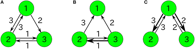
Figure 1. Examples of catalytic reaction networks consisting of 3 species. The rate constants are (A) R₁₂₃ = 1, R₁₃₂ = 1, R₂₁₃ = 1, R₂₃₁ = 1, R₃₁₂ = 1, R₃₂₁ = 0, (B) R₁₂₃ = 0, R₁₃₂ = 0, R₂₁₃ = 1, R₂₃₁ = 1, R₃₁₂ = 2, R₃₂₁ = 1, and (C) R₁₂₃ = 1997/3, R₁₃₂ = 1000/3, R₂₃₁ = 1, R₃₂₁ = 1, R₂₁₃ = 0, R₃₁₂ = 0.

The marginal distributions are shown in Figure 2. Our formula Equation (44) is entirely in agreement with the simulation results. When the total number of molecules N is large, the marginal distributions can be approximated by normal distributions. Similarly, the formulas of the concentrations and the variances, Equations (45a) and (45c), are completely in agreement with the simulation results as shown in Figure 3. One can see that the variances monotonically decrease as N becomes larger.

FIGURE 2

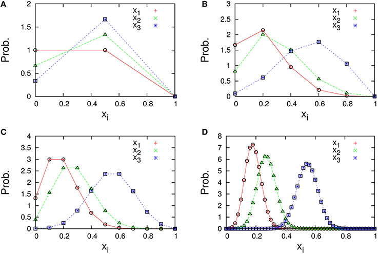
Figure 2. Marginal distributions of x_i = n_i/N (i = 1, 2, 3) in the three-species system of Figure 1A. The total number of molecules in each figure is (A) N = 2, (B) N = 5, (C) N = 10, and (D) N = 50. Cross symbols (red, green, blue) represent the simulation results obtained numerically using the Gillespie algorithm (Gillespie, 1977), which is performed under the following condition; the total number of reactions: 10⁸, the number of reactions for transient exclusion: 10⁷, and the initial value (n₁(0), n₂(0), n₃(0)) is randomly selected from W \ I such that the average per one-species is N/M. Empty symbols (circle, triangle, square) represent the theoretical expression $N{p}_{i*}^{\mathrm{\text{c}}}(Nx)$ [Equation (44)] for λ₁ = 2/11, λ₂ = 3/11, and λ₃ = 6/11.

FIGURE 3

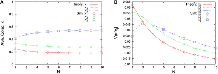
Figure 3. N-dependence of (A) the time-averaged concentrations ${\overline{\mathbf{x}}}_{\mathbf{i}}={\overline{\mathbf{n}}}_{\mathbf{i}}/\mathbf{N}$ and (B) the variances of concentrations $\text{Var}\left[{\mathbf{x}}_{\mathbf{i}}\right]=(\overline{{\mathbf{n}}_{\mathbf{i}}^2}-{\overline{\mathbf{n}}}_{\mathbf{i}}^2)/{\mathbf{N}}^2$ in the three-species system of Figure 1A. Empty symbols are numerically obtained using the Gillespie algorithm, where the time averages are performed over a long time series n_i(t) such that the total number of reactions reaches 10⁸. The initial values are randomly selected from W \ I such that the average per one-species is N/M, and the number of reactions for transient exclusion is 10⁷. Lines in each figure represent the theoretical expressions, Equations (45a) and (45c), for λ₁ = 2/11, λ₂ = 3/11, and λ₃ = 6/11. One can see that the rank of concentrations is conserved but the rank of variances is exchanged between N = 2 and 4.

Note that if the λ-condition (Equation 33) does not have a non-trivial solution like Equation (39), the expression for the PGF (Equation 42) cannot be applied. Such special cases are treated in the following section.

2.4.2.4. Ergodicity as a sufficient condition for applying our PGF

The PGFwoWTAS (Equation 42) would be applicable if the catalytic reaction network was “entirely ergodic,” which means the following in this paper (it is reminiscent of the ω-limit set):

$\begin{array}{ll}\omega ({\mathbf{n}}_0;\xi )=W\backslash I(\forall \xi ),\hfill & (48)\end{array}$

where

$\begin{array}{ll}\omega ({\mathbf{n}}_0;\xi ):={\displaystyle \bigcap _{t\ge 0}}\left\{\mathbf{n}(\tau ;\xi ):\tau \ge t\right\},\hfill & (49)\end{array}$

and ξ represents one of the trials of the stochastic process n(t) according to the catalytic reaction network.

We use a specific three-species system to intuitively illustrate what Equation (48) means. In the case of the three-species system of Figure 1A, the ergodic condition (Equation 48) can be rewritten in terms of simplified conditions. As previously described, the state space of catalytic reaction networks consists of $\left((\frac{M}{N})\right):=\frac{(N+M-1)!}{(M-1)!N!}$ points. Therefore, in the case of M = 3 for example, there are (N + 2)!/(2N!) points. The state space of the three-species system forms a regular triangle in three-dimensional Euclidean space (see Figure 4A). The possible motion from each state point is shown in Figure 4B, where there potentially exist six possible directions, but the network structure forbids the direction of R₃₂₁ in the case of the network of Figure 1A. Note that the state point on the boundary cannot move in a direction parallel to the boundary. In this case obviously, a trajectory starting from an initial point n₀ ∈ W \ I visits every point in W \ I as shown by the circles in Figure 4A (the set I is equivalent to the vertexes of a triangle). Therefore, as seen in Figure 4B, the necessary and sufficient condition to hold the ergodic condition (Equation 48) for M = 3 is:

$\begin{array}{ll}{\displaystyle \sum _{i,j}}{R}_{ijk}>0\&{\displaystyle \sum _{i,j}}{R}_{kij}>0(\forall k),\hfill & (50)\end{array}$

where the first condition represents that at least one direction for moving away from the boundary n_k = 0 is allowed, and the second condition represents that at least one direction for approaching the boundary n_k = 0 is allowed. Note that the condition (Equation 50) is no longer a sufficient condition for entire ergodicity in the case of four-species systems. In fact, in the following four-species system (Figure 5A), the condition (Equation 50) does not imply entire ergodicity;

$\begin{array}{l}{R}_{132}>0,R_{143}>0,R_{231}>0,R_{243}>0,R_{314}>0,\hfill \\ R_{413}>0,(\mathrm{\text{others }}0).\hfill & (51)\end{array}$

This four-species system obviously satisfies the condition (Equation 50), but most initial states [in particular, n_k(0) > 0(∀k)] eventually fall into any of 2-species winners-take-all states, i.e., {n₁ = n₂ = 0, n₃ + n₄ = N}.

FIGURE 4

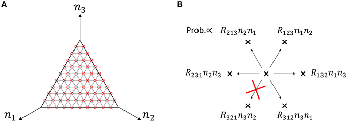
Figure 4. (A) State space of the three-species system of Figure 1A in the case of N = 10. Circles (red) represent the states that a single trajectory can visit, which means that the system is “entirely ergodic.” (B) Motion of the state point when one reaction occurs in the three-species system of Figure 1A. There are 6 possible directions in which to move from one state point. Each direction is randomly selected in proportion to the specified probability. In the case of Figure 1A, the state point cannot move in the direction of R₃₂₁ since R₃₂₁ = 0. Note that the state point on the boundary (e.g., n₁ = 0) cannot move parallel to the boundary (in this case, the directions of R₂₁₃ and R₃₁₂).

FIGURE 5

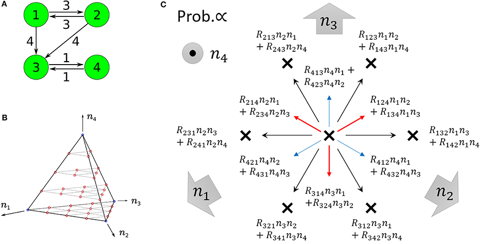
Figure 5. (A) Example of non-ergodic catalytic networks consisting of four species; the rate constants are R₁₃₂ > 0, R₁₄₃ > 0, R₂₃₁ > 0, R₂₄₃ > 0,R₃₁₄ > 0, R₄₁₃ > 0, and others 0. (B) State space of four-species systems in the case of N = 4. Red circles represent the states a single trajectory can visit in the case that the system is entirely ergodic. Blue circles represent winner-takes-all states, i.e., n_k = 4 (∃k). (C) Motion of the state point when one reaction occurs in four-species systems (viewed from the top of B). Red and blue arrows represent upward and downward arrows, respectively. There are 12 possible directions in which to move from one state point. Each direction is randomly selected in proportion to the specified probability. Note that the state point on each $I^{(2)}(i_1,i_2)$ cannot move parallel to itself (e.g., on I⁽²⁾(1, 2), the directions of R₂₃₁, R₂₄₁ as well as R₁₃₂, R₁₄₂ are not allowed).

In the case of M-species systems, a necessary and sufficient condition for entire ergodicity is difficult to derive, although we may consider a sufficient condition instead. We discuss the sufficient condition for entire ergodicity by introducing the collection of all l-species winners-take-all states (l = 1, 2, ⋯ , M):

$\begin{array}{ll}{I}_{M,N}^{(l)}:={\displaystyle \bigcup _{1\le i_1<\cdots <i_l\le M}}{I}_{M,N}^{(l)}(i_1,i_2,\cdots ,i_l),\hfill & (52)\end{array}$

where

$\begin{array}{l}{I}_{M,N}^{(l)}(i_1,i_2,\cdots ,i_l):=\{n\in W_{M,N}\mid n_{i_1}+n_{i_2}+\cdots +n_{i_l}=N\\ \&n_{i_k}>0(\forall k)\}.& (53)\end{array}$

We omit the subscripts M and N provided there is no concern for confusion. The above collections are not empty sets if l ≤ N. Note that I = I⁽¹⁾ and $W={\bigcup }_{l=1}^M{I}^{(l)}$. One can see that the following diagram holds if the catalytic network is fully connected [i.e., R_ijk > 0 for all i, j, k (i ≠ j ≠ k ≠ i)];

$\begin{array}{c}{I}^{(1)}\leftrightarrows ̸I^{(2)}\leftrightarrows I^{(3)}\leftrightarrows \cdots \leftrightarrows I^{(M-1)}\leftrightarrows I^{(M)}\hfill \\ \circlearrowleft \circlearrowleft \circlearrowleft \circlearrowleft \hfill & (54)\end{array}$

where each arrow represents the direction in which a state point can move by one reaction. Each $I^{(l)}(i_1,\cdots ,i_l)$ is a (l−1)-dimensional object in the whole (M − 1)-dimensional state space W. For example, the state space of four-species systems forms a regular tetrahedron W_{M = 4, N} (see Figure 5B); I⁽⁴⁾(1, 2, 3, 4) is the interior of the regular tetrahedron; I⁽³⁾(1, 2, 3), I⁽³⁾(1, 2, 4), I⁽³⁾(1, 3, 4), and I⁽³⁾(2, 3, 4) are regular triangles that form the boundaries of I⁽⁴⁾; and I⁽²⁾(1, 2), I⁽²⁾(1, 3), I⁽²⁾(1, 4), I⁽²⁾(2, 3), I⁽²⁾(2, 4), and I⁽²⁾(3, 4) are line segments that form the boundaries of I⁽³⁾. Note that $I^{(2)}(i_1,i_2)\to I^{(2)}(j_1,j_2)$ for (i₁, i₂) ≠ (j₁, j₂) is possible but $I^{(2)}(i_1,i_2)\to I^{(2)}(i_1,i_2)$ is always impossible as seen from Figure 5C. By considering the diagram (Equation 54) and keeping in mind Figures 5B,C, we can expect the following fact: if entire ergodicity holds in the restricted system on I^(l) for l ≥ 3, then entire ergodicity holds in the whole state space W. In other words, in systems consisting of M-species, the sufficient condition under which the ergodic condition (Equation 48) holds can be geometrically described as follows: on each $I^{(l)}(i_1,\cdots ,i_l)$ for l ≥ 3, at least one direction for moving away from each boundary $I^{(l-1)}(j_1,\cdots ,j_{l-1})$ should be allowed, and simultaneously at least one direction for approaching each boundary $I^{(l-1)}(j_1,\cdots ,j_{l-1})$ should also be allowed, where {j₁, ⋯ , j_l−1}⊂{i₁, ⋯ , i_l}.

2.4.3. The Case of Catalytic-Noncatalytic Mixed Reactions

We could not obtain the steady-state solution of the general GFE (Equation 11) in the case of catalytic-noncatalytic mixed reactions (ε > 0), but we expect our PGF (Equation 42) to be a good approximation for mixed-reaction systems if ε is sufficiently small (ε ≪ min{R_ijk > 0}). More specifically, we expect the PGF (Equation 42) to be robust against non-catalytic reactions if the catalytic reaction system constituting the mixed reaction system has an ergodic component spread across the entire state space (entire ergodicity). Otherwise, if the catalytic reaction system has several ergodic components in the entire state space, the non-catalytic reactions may imply that a certain highly stable ergodic component attracts all possible trajectories, which obviously means that our PGF is not applicable to such a mixed reaction system. Although we were unable to prove this mathematically, we used numerical simulations to determine whether our PGF is a good approximation in the case of “entirely ergodic.”

Figure 6 represents the non-catalytic reaction rate constant ε dependencies of time-averaged concentrations x_i for the three-species system of Figures 1A,B. (As shown later, the system shown in Figure 1B is not entirely ergodic, which is the reason why the systems shown in Figures 1A,B are compared here.) It can be seen that the differences of x_i in Figure 6A between ε = 0 and ε = 0.1 are smaller than those in Figure 6B. We consider the robustness in the case of Figure 6A to originate from the entire ergodicity of Figure 1A, which means that the ergodic component spreads on the entire state space except for winner-takes-all states (see Figure 4A).

FIGURE 6

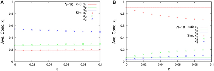
Figure 6. ε-dependence of the time-averaged concentrations x_i (N = 10, ρ = 1) in the case of (A) the three-species system of Figure 1A with non-catalytic reactions and (B) that of Figure 1B with non-catalytic reactions. Points in the figures are numerically obtained using the Gillespie algorithm in the same way as Figure 3. The catalytic reaction network of Figure 1A is entirely ergodic; thus, the non-catalytic reactions may be treated as perturbation. On the other hand, that of Figure 1B is non-ergodic; thus, the non-catalytic reactions introduce relatively large differences compared with the case of ε = 0.

3. Applications

The starting point of our analysis is the GFE (Equation 11), from which several useful formulas are derived, namely the PRE (Equation 15), SME (Equation 18), TESMs (Equation 19) and (Equation 20), the λ-condition (Equation 33), and the PGFwoWTAS (Equation 42). In this section, we reveal the effectiveness of these formulas by showing important applications for several catalytic reaction networks.

3.1. Rank Conservation Law for Concentrations

We show that the rank of concentrations is conserved even if the total number of molecules changes in catalytic reaction networks (excluding non-catalytic and auto-catalytic reactions).

Suppose the concentration of the ith-species is expressed by Equation (45a) in the state corresponding to the PGFwoWTAS. When determining the rank conservation, it suffices to confirm that the relation between the amount of two arbitrary species is unchanged if the total number of molecules is changed. Let λ₁, λ₂ be the concentrations per total density in the continuous limit such that λ₁ < λ₂. Because $\sum _{i=1}^M{\lambda }_i=1$, the inequality λ₁ + λ₂ < 1 must be satisfied. Therefore, the following evaluation holds:

$\begin{array}{l}{\overline{x}}_2-{\overline{x}}_1=\frac{({\lambda }_2-{\lambda }_2^N)-({\lambda }_1-{\lambda }_1^N)}{1-{\displaystyle {\sum }_{i=1}^M{\lambda }_i^N}}\rho \\ =\frac{({\lambda }_2-{\lambda }_1)\rho }{1-{\displaystyle {\sum }_{i=1}^M{\lambda }_i^N}}[1-{({\lambda }_2+{\lambda }_1)}^{N-1}\\ +{\displaystyle \sum _{k=1}^{N-2}\left\{\left(\begin{array}{c}N-1\\ k\end{array}\right)-1\right\}}{\lambda }_2^{N-1-k}{\lambda }_1^k]\\ >0(\forall N\in {\mathbb{N}}_{\ge 2}).& (55)\end{array}$

This is the rank conservation law of concentrations.

Note that the rank of the variances of concentrations is generally not conserved when the total number of molecules changes. For example, let us consider the following three-species system (Figure 1C);

$\begin{array}{l}{R}_{123}=1997/3,R_{132}=1000/3,R_{231}=R_{321}=1,\hfill \\ R_{213}=R_{312}=0;\rho =1.\hfill & (56)\end{array}$

As shown in Figure 7, this system depends on the total number of molecules for the time-averaged concentrations ${\overline{x}}_i$ and the variances of concentrations Var[x_i], represented by Equations (45a) and (45c) with λ₁ = 1/1000, λ₂ = 1/3, and λ₃ = 1997/3000. The rank of time-averaged concentrations is always conserved, but the rank of variances is exchanged at certain N (see Figure 8).

FIGURE 7

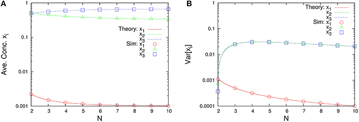
Figure 7. N-dependence of (A) the time-averaged concentrations ${\overline{\mathbf{x}}}_{\mathbf{i}}={\overline{\mathbf{n}}}_{\mathbf{i}}/\mathbf{N}$ and (B) the variances of concentrations $\text{Var}\left[{\mathbf{x}}_{\mathbf{i}}\right]=(\overline{{\mathbf{n}}_{\mathbf{i}}^2}-{\overline{\mathbf{n}}}_{\mathbf{i}}^2)/{\mathbf{N}}^2$ in the three-species system of Figure 1C. Empty symbols are numerically obtained using the Gillespie algorithm in the same way as Figure 3. Lines in each figure represent the theoretical expressions, Equations (45a) and (45c), for λ₁ = 1/1000, λ₂ = 1/3, and λ₃ = 1997/3000. It is clear that the rank of time-averaged concentrations is conserved.

FIGURE 8

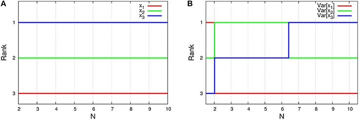
Figure 8. N-dependence of (A) the rank of time-averaged concentrations and (B) the rank of its variances in the three-species system of Figure 1C. The ranks (lines) in the figures are depicted using the formulas (Equations 45a and 45c). Clearly, the rank of concentrations is conserved, although the rank of variances is exchanged between N = 2 and 3, and also N = 6 and 7.

3.2. A Special Case: The Connecting State to the Winner-Takes-All State

There exists an N-molecular state, which connects to the winner-takes-all state in the continuous limit N → ∞. As is later shown, such a special case is not the “weakly reversible” case (Anderson et al., 2010).

We show this by taking the following limit in the PGFwoWTAS (Equation 42):

$\begin{array}{ll}{\lambda }_1\to 1,{\lambda }_2,\cdots ,{\lambda }_M\to 0,\hfill & (57)\end{array}$

where we suppose the following constraints are always satisfied:

$\begin{array}{ll}\frac{{\lambda }_i}{{\lambda }_2+{\lambda }_3+\cdots +{\lambda }_M}={\kappa }_i(i=2,3,\cdots ,M),\hfill & (58)\end{array}$

where {κ_i} are positive constants, which are determined from the network structure {R_ijk} (it is explained later). Evidently, the following holds;

$\begin{array}{ll}{\displaystyle \sum _{i=2}^M}{\kappa }_i=1.\hfill & (59)\end{array}$

The PGFwoWTAS (Equation 42) has the following limiting expression:

$\begin{array}{l}{\varphi }_{*}^{\mathrm{\text{c}}}(\mathbf{z})=\frac{{\left(\frac{{\lambda }_1}{1-{\lambda }_1}{z}_1+{\displaystyle {\sum }_{i=2}^M}{\kappa }_i{z}_i\right)}^N-{\left(\frac{{\lambda }_1}{1-{\lambda }_1}{z}_1\right)}^N-{\displaystyle {\sum }_{i=2}^M}{\left({\kappa }_i{z}_i\right)}^N}{{\left(\frac{1}{1-{\lambda }_1}\right)}^N-{\left(\frac{{\lambda }_1}{1-{\lambda }_1}\right)}^N-{\displaystyle {\sum }_{i=2}^M}{\kappa }_i^N},\hfill \\ {\displaystyle \underset{{\lambda }_1\to 1}{\overset{}{\to }}}{z}_1^{N-1}\left({\kappa }_2{z}_2+\cdots +{\kappa }_M{z}_M\right)\equiv {\varphi }_{*}^{\mathrm{\text{cs}}}(\mathbf{z}).\hfill & (60)\end{array}$

The state corresponding to the PGF (Equation 60) is the connecting state to the winner-takes-all state (CStoWTAS). The stationary distribution corresponding to the CStoWTAS is immediately obtained:

$\begin{array}{ll}{P}_{*}^{\text{cs}}(\mathbf{n})=\{\begin{array}{l}{\kappa }_i (\mathbf{n}\in J),\\ 0 (\mathbf{n}\in W\backslash J),\hfill \end{array}\hfill & (61)\end{array}$

where J_{M, N} (abbr. J) is defined as

$\begin{array}{ll}J=\left\{\mathbf{n}\in W_{M,N}\mid n_1=N-1 \exists i\in \left[2,M\right]\text{ s.t. }{n}_i=1\right\}.\hfill & (62)\end{array}$

Furthermore, the marginal distributions of the i-th species can be derived by Equation (13):

$\begin{array}{l}{p}_{i\ast }^{\text{cs}}(n)=\{\begin{array}{ll}{\delta }_{n,N-1}\hfill & \text{for\hspace{1em}}i=1,\hfill \\ (1-{\kappa }_i){\delta }_{n,0}+{\kappa }_i{\delta }_{n,1}\hfill & \text{for\hspace{1em}}i=2,\cdots ,M,\hfill \end{array}\\ (0\le n\le N),& (63)\end{array}$

where δ_ij is the Kronecker delta, δ_ij = 0 (if i ≠ j) or 1 (if i = j). The time-averaged concentrations calculated by Equation (12) are

$\begin{array}{ll}{\overline{x}}_1=\left(1-\frac{1}{N}\right)\rho ,\hfill & (\mathrm{64a})\end{array}$

$\begin{array}{ll}{\overline{x}}_i=\frac{{\kappa }_i}{N}\rho (i=2,\cdots ,M),\hfill & (\mathrm{64b})\end{array}$

and the variances of the time-averaged concentrations calculated by Equation (12) are

$\begin{array}{ll}\text{Var}\left[x_1\right]=0,\hfill & (\mathrm{65a})\end{array}$

$\begin{array}{ll}\text{Var}\left[x_i\right]=\frac{{\kappa }_i(1-{\kappa }_i)}{N^2}{\rho }^2(i=2,\cdots ,M).\hfill & (\mathrm{65b})\end{array}$

Next, we derive the relation between the positive constants {κ_i} and the network structure {R_ijk}. The λ-condition (Equation 33) can be converged to conditions for {κ_i} (the κ-condition) by taking the limit λ₁ → 1 as follows. Divide the λ-condition (Equation 33) into two groups, of which one group is the case of 2 ≤ i < j ≤ M,

$\begin{array}{l}{R}_{1ij}{\lambda }_1{\kappa }_i+R_{1ji}{\lambda }_1{\kappa }_j-\left(R_{ij1}+R_{ji1}\right){\kappa }_i{\kappa }_j(1-{\lambda }_1)\hfill \\ +(1-{\lambda }_1){\displaystyle \sum _{k=2}^M}\left\{R_{kij}{\kappa }_k{\kappa }_i+R_{kji}{\kappa }_k{\kappa }_j-\left(R_{ijk}+R_{jik}\right){\kappa }_i{\kappa }_j\right\}=0,\hfill & (\mathrm{66a})\end{array}$

and the other group is the case of i = 1, 2 ≤ j ≤ M,

$\begin{array}{ll}{\displaystyle \sum _{k=2}^M}\left\{R_{k1j}{\kappa }_k{\lambda }_1+R_{kj1}{\kappa }_k{\kappa }_j(1-{\lambda }_1)-\left(R_{1jk}+R_{j1k}\right){\lambda }_1{\kappa }_j\right\}=0,\hfill & (\mathrm{66b})\end{array}$

where we substituted λ_i = κ_i(1− λ ₁), i ≥ 2 and divided by 1− λ ₁. Then, taking the limit λ₁ → 1 in Equation (66a),

$\begin{array}{ll}{\kappa }_i{R}_{1ij}+{\kappa }_j{R}_{1ji}=0\text{\hspace{1em} i.e., }{R}_{1ij}=0(\forall i,j),\hfill & (\mathrm{67a})\end{array}$

and taking that in Equation (66b),

$\begin{array}{ll}{\displaystyle \sum _{k=2}^M}\left({\kappa }_k{R}_{k1j}-{\kappa }_j{R}_{j1k}\right)=0(2\le j\le M).\hfill & (\mathrm{67b})\end{array}$

The condition (Equation 67a) expresses that the 1st-species cannot be a substrate, and the condition (Equation 67b) represents the desired κ-condition. Note that the CStoWTAS must be a limiting state corresponding to the PGFwoWTAS [see Equation (60)]. Therefore, the network structure {R_ijk} must have definite {λ_i}.

For example, let us consider the following three-species system (Figure 1B):

$\begin{array}{ll}{R}_{123}=R_{132}=0,R_{213}=R_{231}=R_{321}=1,R_{312}=2;\rho =1,\hfill & (68)\end{array}$

which implies κ₂ = 2/3 and κ₃ = 1/3. Obviously, this system is not weakly reversible, which means that the theorems (Theorem 4.1 and 4.2) in the previous study (Anderson et al., 2010) cannot be applied. This system should have a CStoWTAS because λ₁, λ₂, and λ₃ are definite from Equation (39) with Λ₁ = 0, Λ₂ = 2, and Λ₃ = 4. As shown in Figure 9, this system certainly has the time-averaged concentrations ${\overline{x}}_i$ represented by Equation (64) and the variances Var[x_i] represented by Equation (65). In this case also, the rank conservation law of concentrations holds.

FIGURE 9

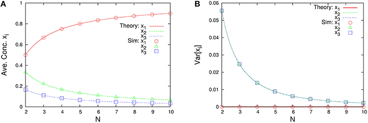
Figure 9. N-dependence of (A) time-averaged concentrations ${\overline{\mathbf{x}}}_{\mathbf{i}}={\overline{\mathbf{n}}}_{\mathbf{i}}/\mathbf{N}$ and (B) the variances of concentrations $\text{Var}\left[{\mathbf{x}}_{\mathbf{i}}\right]=(\overline{{\mathbf{n}}_{\mathbf{i}}^2}-{\overline{\mathbf{n}}}_{\mathbf{i}}^2)/{\mathbf{N}}^2$ in the three-species system of Figure 1B. Empty symbols were numerically obtained using the Gillespie algorithm in the same way as Figure 3. Lines in each figure represent the theoretical expressions, Equations (64) and (65), for κ₂ = 2/3 and κ₃ = 1/3.

3.3. M-Species 2-Molecules Systems with Non-catalytic Reactions

The 2mTESM (Equation 20) becomes the closed equation of the second-order moments 〈x_lx_m〉 if the first-order moments 〈x_i〉 are substituted by the second-order moments according to the PRE (Equation 20). In this subsection, we consider catalytic-non-catalytic mixed reaction systems of M species, consisting of only 2 molecules in total.

We first focus on the second formula in the 2mTESMs (Equation 20). It can be seen that each variance of time-averaged concentration $\text{Var}\left[x_i\right]=\overline{x_i^2}-{\overline{x_i}}^2$ in the steady state depends solely on its concentration:

$\begin{array}{ll}\text{Var}\left[x_i\right]=\left(\frac{M+1}{2M}\rho -{\overline{x}}_i\right){\overline{x}}_i,\hfill & (69)\end{array}$

where we supposed the ergodicity $\langle x_i\rangle ={\overline{x}}_i$. The above equation expresses that the fluctuation of the concentration x_i becomes larger as its time-averaged concentration approaches

$\begin{array}{ll}\overline{x}=\frac{M+1}{4M}\rho ,\hfill & (70)\end{array}$

at which the fluctuation takes the largest value ${\left(\frac{M+1}{4M}\rho \right)}^2$. Furthermore, the time-averaged concentrations potentially have the maximum value because the variance must be positive;

$\begin{array}{ll}{\overline{x}}_i\le \frac{M+1}{2M}\rho (\forall i\in \left[1,M\right]).\hfill & (71)\end{array}$

Next, we focus on the first formula in the 2mTESMs (Equation 20). Let us consider the steady state of Equation (20a) and suppose the ergodicity $\langle x_i\rangle ={\overline{x}}_i$. Eliminating the first-order moments in Equation (20a) by using the SME (Equation 18) gives the determination equation of second-order moments in the 2 molecules system (2mDESM);

$\begin{array}{l}\frac{4\epsilon }{\rho }\overline{x_l{x}_m}+{\displaystyle \sum _i}\left\{\left(R_{lmi}+R_{mli}\right)\overline{x_l{x}_m}-R_{ilm}\overline{x_i{x}_l}-R_{iml}\overline{x_i{x}_m}\right\}\hfill \\ -\frac{1}{M}{\displaystyle \sum _{ij}}\left\{\left(R_{jil}+R_{jim}\right)\overline{x_i{x}_j}-R_{lij}\overline{x_i{x}_l}-R_{mij}\overline{x_i{x}_m}\right\}\hfill \\ =\frac{2\rho \epsilon }{M^2}(1\le l<m\le M).\hfill & (72)\end{array}$

The above 2mDESM can be rewritten in the M(M−1)/2 × M(M−1)/2 matrix form. We demonstrate the procedure for processing the 2mDESM by considering the case of M = 3. In this case, the 2mDESM (Equation 72) has a matrix of the following form:

$\begin{array}{l}\left[\begin{array}{ccc}\frac{4}{3}(R_{123}+R_{213})+\text{}\frac{4\epsilon }{\rho }& \text{}-\frac{4}{3}{R}_{312}& \text{}-\frac{4}{3}{R}_{321}\\ -\frac{4}{3}{R}_{213}& \text{}\frac{4}{3}(R_{132}+R_{312})+\text{}\frac{4\epsilon }{\rho }& \text{}-\frac{4}{3}{R}_{231}\\ -\frac{4}{3}{R}_{123}& \text{}-\frac{4}{3}{R}_{132}& \text{}\frac{4}{3}(R_{231}+R_{321})+\text{}\frac{4\epsilon }{\rho }\end{array}\right]\\ \left[\begin{array}{c}\overline{x_1{x}_2}\\ \overline{x_1{x}_3}\\ \overline{x_2{x}_3}\end{array}\right]=\frac{2\rho \epsilon }{9}\left[\begin{array}{c}1\\ 1\\ 1\end{array}\right].& (73)\end{array}$

Moreover, we consider the specific three-species system of Figure 1A (ρ = 1) including non-catalytic reactions. Solving Equation (73) as ε > 0 and ρ = 1 in the case of Figure 1A, then

$\begin{array}{ll}\left[\begin{array}{c}\overline{x_1{x}_2}\\ \overline{x_1{x}_3}\\ \overline{x_2{x}_3}\end{array}\right]=\left[\begin{array}{c}\frac{1+3\epsilon }{18(2+3\epsilon )}\\ \frac{1}{18}\\ \frac{1+\epsilon }{6(2+3\epsilon )}\end{array}\right],\hfill & (74)\end{array}$

which is consistent with the result obtained when solving the CME (Equation 7) directly [recall $\langle x_1{x}_2\rangle =\frac{1}{4}P(n_1=1,n_2=1,n_3=0)$, 〈x₁x₃〉 = ⋯  and so on]. By the SME (Equation 18), the concentrations become

$\begin{array}{ll}{\overline{x}}_1=\frac{1+2\epsilon }{2(2+3\epsilon )},{\overline{x}}_2=\frac{1}{3},{\overline{x}}_3=\frac{5+6\epsilon }{6(2+3\epsilon )}.\hfill & (75)\end{array}$

Figure 10 shows the second-order moments $\overline{x_i{x}_j}$ and the time-averaged concentrations ${\overline{x}}_i$ as functions of ε. Note that in the case of ε = 0 (catalytic reactions only), we need to derive the second-order moments $\overline{x_i{x}_j}$ from Equation (45b) corresponding to λ₁ = 2/11, λ₂ = 3/11, and λ₃ = 6/11. The non-catalytic reaction rate constant ε seems to be a singular perturbation against the second-order moments (not the concentrations).

FIGURE 10

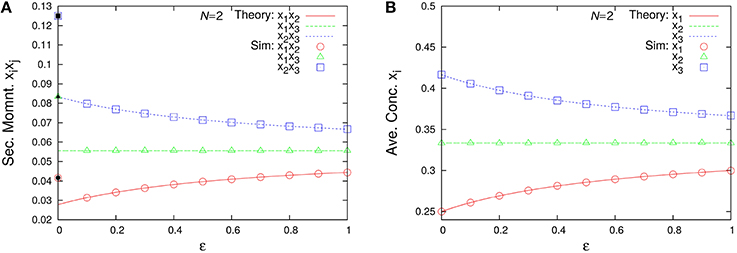
Figure 10. ε-dependence of (A) the second-order moments $\overline{{\mathbf{x}}_{\mathbf{i}}{\mathbf{x}}_{\mathbf{j}}}=\overline{{\mathbf{n}}_{\mathbf{i}}{\mathbf{n}}_{\mathbf{j}}}/{\mathbf{N}}^2$ and (B) the time-averaged concentrations ${\overline{\mathbf{x}}}_{\mathbf{i}}={\overline{\mathbf{n}}}_{\mathbf{i}}/\mathbf{N}$ in the three-species system of Figure 1A with non-catalytic reactions (N = 2, ρ = 1). Empty symbols are numerically obtained using the Gillespie algorithm in the same way as Figure 3. Lines in each figure represent the theoretical expressions, Equations (74) and (75). Note that there exist differences between the limit ε → 0 and the case ε = 0 for the second-order moments (solid black points) because the SME (Equation 18) breaks down at ε = 0. The solid black points are calculated from Equation (45b) as λ₁ = 2/11, λ₂ = 3/11, λ₃ = 6/11, N = 2, and ρ = 1.

3.4. Non-autocatalyzation of Autocatalytic Reaction Networks

The framework we developed in this paper applies to non-autocatalytic reaction networks. However, our framework may be applicable to autocatalytic reaction networks if it were possible to convert autocatalytic to non-autocatalytic networks. Here, we show several examples of such conversions using a minimal autocatalytic reaction network “2TK model” (Ohkubo et al., 2008; Saito and Kaneko, 2015), which is a well-studied model in the context of discreteness-induced phenomena.

The 2TK model consists of only two species, and includes both autocatalytic reactions (rate const. r) and non-catalytic reactions (rate const. ε ≪ r) (see Figure 11A);

$\begin{array}{ll}A\stackrel{B}{{\displaystyle \underset{A}{\rightleftarrows }}}B(\mathrm{\text{autocat. react.}}),\hfill & (76)\end{array}$

$\begin{array}{ll}A\rightleftarrows B(\mathrm{\text{non-cat. react.}}).\hfill & (77)\end{array}$

If we suppose that each of the species A and B consists of two further species, we can convert autocatalytic reactions Equation (76) of the 2TK model to non-autocatalytic reactions as shown in Figure 11B. The catalysis of the species 5 between the species 1 and 3 (or, 2 and 4) is to establish an equilibrium between the concentrations of the species 1 and 3 (or, 2 and 4), that would make it possible to regard these as one species. The non-autocatalytic reactions of Figure 11B plus non-catalytic reactions $i\underset{}{\overset{\mathrm{\text{Prob.}}1/5}{\to }}j$ is the desired five-component model, of which the CME is simply described by Equation (7) with

$\begin{array}{ll}{R}_{142}=R_{153}=R_{231}=R_{254}=R_{351}=R_{452}=1(\mathrm{\text{others }}0).\hfill & (78)\end{array}$

As shown in Figure 12, the behavior of the variables n_A = n₁+n₃+n₅/2 and n_B = n₂+n₄+n₅/2 in the five-component model is similar to that of the 2TK model (compare with Figures 1A,B in Saito and Kaneko, 2015). The λ-condition (Equation 33) of catalytic reactions in the five-component model can be written in matrix form,

$\begin{array}{ll}\left[\begin{array}{cccccccccc}0& 0& 0& 0& 0& 0& 0& 0& 0& 0\\ 0& 0& 0& 0& 1& 0& 0& 0& 0& 0\\ 0& 0& -1& 0& 0& 0& 0& 0& 0& 0\\ 0& 0& 0& -1& 0& 0& 0& 0& 1& 0\\ 0& 0& 0& 0& -1& 0& 0& 0& 0& 0\\ 0& 0& 1& 0& 0& 0& 0& 0& 0& 0\\ 0& 0& 0& 0& 0& 0& -1& 0& 0& 1\\ 0& 0& 0& 0& 0& 0& 0& 0& 0& 0\\ 0& 0& 0& 1& 0& 0& 0& 0& -1& 0\\ 0& 0& 0& 0& 0& 0& 1& 0& 0& -1\end{array}\right]\left[\begin{array}{c}{\lambda }_1{\lambda }_2\\ {\lambda }_1{\lambda }_3\\ {\lambda }_1{\lambda }_4\\ {\lambda }_1{\lambda }_5\\ {\lambda }_2{\lambda }_3\\ {\lambda }_2{\lambda }_4\\ {\lambda }_2{\lambda }_5\\ {\lambda }_3{\lambda }_4\\ {\lambda }_3{\lambda }_5\\ {\lambda }_4{\lambda }_5\end{array}\right]=0,\hfill & (79)\end{array}$

in which there exist six non-trivial eigenvectors corresponding to the 0-eigenvalue; hence, the general eigenvector corresponding to the 0-eigenvalue can be expressed as a linear summation of those six non-trivial eigenvectors:

$\begin{array}{ll}\left[\begin{array}{c}{\lambda }_1{\lambda }_2\\ {\lambda }_1{\lambda }_3\\ {\lambda }_1{\lambda }_4\\ {\lambda }_1{\lambda }_5\\ {\lambda }_2{\lambda }_3\\ {\lambda }_2{\lambda }_4\\ {\lambda }_2{\lambda }_5\\ {\lambda }_3{\lambda }_4\\ {\lambda }_3{\lambda }_5\\ {\lambda }_4{\lambda }_5\end{array}\right]=c_1\left[\begin{array}{c}1\\ 0\\ 0\\ 0\\ 0\\ 0\\ 0\\ 0\\ 0\\ 0\end{array}\right]+c_2\left[\begin{array}{c}0\\ 1\\ 0\\ 0\\ 0\\ 0\\ 0\\ 0\\ 0\\ 0\end{array}\right]+c_3\left[\begin{array}{c}0\\ 0\\ 0\\ 0\\ 0\\ 1\\ 0\\ 0\\ 0\\ 0\end{array}\right]+c_4\left[\begin{array}{c}0\\ 0\\ 0\\ 0\\ 0\\ 0\\ 0\\ 1\\ 0\\ 0\end{array}\right]+c_5\left[\begin{array}{c}0\\ 0\\ 0\\ 1\\ 0\\ 0\\ 0\\ 0\\ 1\\ 0\end{array}\right]+c_6\left[\begin{array}{c}0\\ 0\\ 0\\ 0\\ 0\\ 0\\ 1\\ 0\\ 0\\ 1\end{array}\right].\hfill & (80)\end{array}$

The above equation can be used to derive six types of non-trivial solutions (λ₁, λ₂, ⋯ , λ₅), which immediately correspond to the stationary states of catalytic reactions in the five-component model by using Equation (43):

$\begin{array}{ll}({\lambda }_1,{\lambda }_2,{\lambda }_3,{\lambda }_4,{\lambda }_5)=\{\begin{array}{ll}\text{(i)}\hfill & (0,c,0,c,1-2c),\hfill \\ \text{(ii)}\hfill & (c,0,c,0,1-2c),\hfill \\ \text{(iii)}\hfill & (2c,1-2c,0,0,0),\hfill \\ \text{(iv)}\hfill & (2c,0,1-2c,0,0),\hfill \\ \text{(v)}\hfill & (0,2c,0,1-2c,0),\hfill \\ \text{(vi)}\hfill & (0,0,2c,1-2c,0),\hfill \end{array}\forall c\in (0,1/2),\hfill & (81)\end{array}$

where each case (i-vi) corresponds to (i) $c_3=c^2$, c₆ = c(1−2c) (others 0), (ii) $c_2=c^2$, c₅ = c(1−2c) (others 0), (iii) c₁ = 2c(1−2c) (others 0), (iv) c₂ = 2c(1−2c) (others 0), (v) c₃ = 2c(1−2c) (others 0), and (vi) c₄ = 2c(1−2c) (others 0). The switching behavior of the five-component model may be explained in terms of transition processes between the above six types of steady states and the five trivial steady states λ_i = 1 (others 0) of catalytic reactions in the five-component model, which are sometimes caused by non-catalytic reactions. Furthermore, the marginal distribution of the species A, p_A(n), can be derived by calculating the convolution of the marginal distributions p₁(n), p₃(n), and p₅(n), if p₁(n), p₃(n), and p₅(n) were obtained for the case including non-catalytic reactions.

FIGURE 11

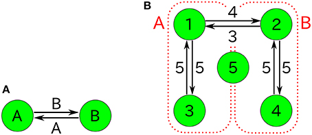
Figure 11. (A) Autocatalytic reactions constituting the 2TK model and (B) five-component non-autocatalytic reactions duplicating the behavior of the 2TK model; R₁₄₂ = R₁₅₃ = R₂₃₁ = R₂₅₄ = R₃₅₁ = R₄₅₂ = 1 (others 0). If one regards the species 1, 3, and half of 5 as the species A (similarly, 2, 4, and half 5 as B), the behavior of n_A = n₁+n₃+n₅/2 and n_B = n₂+n₄+n₅/2 is similar to that of the 2TK model.

FIGURE 12

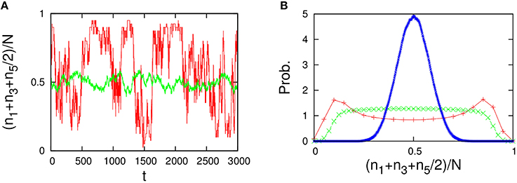
Figure 12. Behavior of the five-component model [Figure 11B plus non-catalytic reactions (ε = 0.01, ρ = 1)]. The behavior of the five-component model is reminiscent of the behavior of the 2TK model (compare with Figures 1A,B in Saito and Kaneko, 2015). (A) Time series of the total concentration of the species 1, 3, and half of 5 for N = 20 (red line) and N = 2000 (green line). (B) Stationary distributions of (n₁+n₃+n₅/2)/N, obtained numerically from a long time series n_i(t) using the Gillespie algorithm whose simulation conditions are the total number of reactions: 10⁸, the number of reactions for transient exclusion: 10⁷, and the initial value is randomly selected from W \ I such that the average per one-species is N/M. The unimodal distribution (blue), the flat distribution (green), and the bimodal distribution (red) indicate the stationary distribution for N = 500, 40, and 20, respectively.

Other non-autocatalytic reaction networks duplicating the 2TK model are shown in Figure 13A, and consist of 4 components only. Although readers would think that the four-component models do not function properly because the transitions between the species group (1, 3) [or (2, 4)] depend on the other species group (2, 4) [or (1, 3)], the four-component models actually generate much the same behavior with the 2TK model (see Figure 14). The switching behavior of the four-component model may also be explained as a transition process between the following three types of steady states

$\begin{array}{ll}({\lambda }_1,{\lambda }_2,{\lambda }_3,{\lambda }_4)=\{\begin{array}{l}(0,0,c,1-c),\hfill \\ (0,c,0,1-c),\hfill \\ (c,0,1-c,0),\hfill \end{array}\forall c\in (0,1),\hfill & (82)\end{array}$

and the four trivial steady states λ_i = 1 (others 0) of catalytic reactions in the four-component model, which are sometimes caused by non-catalytic reactions. We also confirmed that the results are not changed even in the other four-component model of Figure 13B, of which the catalysis role of each the species 1 and 2 is exchanged by that of 3 and 4, respectively.

FIGURE 13

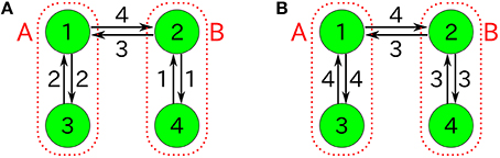
Figure 13. Four-component non-autocatalytic reactions duplicating behaviors of the 2TK model; (A) R₁₂₃ = R₁₄₂ = R₂₁₄ = R₂₃₁ = R₃₂₁ = R₄₁₂ = 1 (others 0), and (B) R₁₄₂ = R₁₄₃ = R₂₃₁ = R₂₃₄ = R₃₄₁ = R₄₃₂ = 1 (others 0). If one regards the species 1 and 3 as the species A (similarly, 2 and 4 as B), the behavior of n_A = n₁+n₃ and n_B = n₂+n₄ is almost equivalent to that of the 2TK model.

FIGURE 14

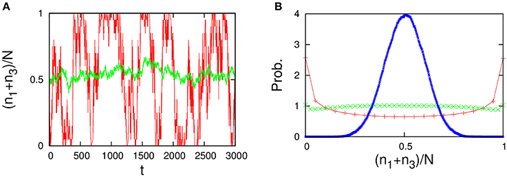
Figure 14. Behavior of the four-component model [Figure 13A plus non-catalytic reactions (ε = 0.01, ρ = 1)]. The four-component model reproduces the behavior of the 2TK model (compare with Figures 1A,B in Saito and Kaneko, 2015). (A) Time series of the total concentration of the species 1 and 3 for N = 20 (red line) and N = 2000 (green line). (B) Stationary distributions of (n₁+n₃)/N, obtained numerically from a long time series n_i(t) using the Gillespie algorithm in the same way as Figure 12. The unimodal distribution (blue), the uniform distribution (green), and the bimodal distribution (red) indicate the stationary distribution for N = 500, 40, and 20, respectively.

4. Summary and Discussions

The framework we presented in this paper facilitates the prediction of the effect of the small-number issue on the concentration of each species in catalytic reaction networks. This can be described in an extreme manner by comparing the concentrations between the continuous limit (N → ∞) and the case of 2 molecules (N = 2). If the reaction network does not include non-catalytic reactions (or, includes negligible non-catalytic reactions), we can use the formula (Equation 45a) to compare them. On the other hand, if the reaction network includes (non-negligible) non-catalytic reactions, we need to apply the formula, 2mDESM (Equation 72), with the SME (Equation 18) to obtain the concentrations in the case of 2 molecules. Although our theory has a presupposition referred to as entire ergodicity, the presupposition is intuitively verifiable if the system is specified, as in Section 2.4.2.4. We also demonstrated three examples for non-autocatalyzation conversions of autocatalytic reaction networks in Section 3.4. We consider this type of conversion to be generalized relatively easily such that our analytical framework can be applied to more general catalytic reaction networks including autocatalytic reactions.

One might think that the analysis presented in this paper can be straightforwardly extended to the case including autocatalytic reactions [in fact, the CME (Equation 7) and GFE (Equation 11) themselves hold even in the case including autocatalytic reactions]. However, if autocatalytic reactions are included (i.e., the case R_ikk > 0 is allowed), we cannot consider catalytic reactions and non-catalytic reactions to be completely separate. The reason is that, in the case including autocatalytic reactions, the absence of non-catalytic reactions generally implies winner-takes-all steady states. Generally, solving the CME (or GFE) of catalytic-noncatalytic mixed reactions systems is more advanced and a more difficult task than that of catalytic reactions only. The proposed strategy, i.e., non-autocatalyzation conversions, is one of our ideas to address the problem.

The formulas obtained in the present work are specific and satisfactorily simple. Therefore, our theory has the capabilities to be developed into a general theory for catalytic reaction networks. On the other hand, there exists a mathematical theory for a certain class of catalytic reaction networks that are “weakly reversible” and “deficiency zero” (Anderson et al., 2010). Our formulas (Equations 27 and 43) are consistent with the main theorems (theorem 4.1 and 4.2 in Anderson et al., 2010) in the above-mentioned mathematical theory. One of the advantages of our theory compared to the above mathematical theory is understandably the probability generating function (PGF) approach, because the PGF is a major analytical tool for physicists, chemists, and mathematical biologists. Therefore, our theory is easily verifiable, and one can design a computer algorithm to calculate our analytical formulas. We also showed the extensibility of our theory by using applications (in Section 3), especially because of the CStoWTAS (Equation 61), which was not suggested by the above mathematical theory.

Actual biochemical pathways in the cell involve thousands of chemical species, and their chemical properties vary. Our theoretical framework is general and extensible to such complex reaction networks, if they can be represented by CMEs such as Equation (7). As our current model consists of simple two-body catalytic reactions, it is difficult to point out examples in actual biological systems that correspond exactly to our model. Biochemical reactions in reality may involve a number of intermediates. There are also autocatalytic processes such as autophosphorylation, and replication of templates such as DNA, in which the catalyst or template species is also a substrate or a product. Our framework is applicable to many such cases involving network conversion, as shown for simple autocatalytic cases.

Nevertheless, the reaction kinetics of each enzyme is not always simple. Enzymes are complex macromolecules and their reaction cycles may depend on their conformational states. Therefore, the prediction of biological phenomena caused by small-number effects in real biochemical reactions, would entail further analytical challenges for catalytic reaction networks including arbitrary higher-order mixed reactions (rather than first- and second-order reactions only) or internal dynamics of the enzymes (as modeled and analyzed in Togashi and Casagrande, 2015) as important issues.

Throughout this work, our primary intention is to approach small-number issues in biological systems. One might wonder how general these small-number issues appear, and how important they are, in living cells. Recently, absolute quantification of various proteins and mRNAs in the cell has become possible, and the integration of experimental results (e.g., the construction of a database Milo et al., 2010) is also underway. Taniguchi et al. investigated the copy number distribution for more than a thousand protein species in bacteria (Taniguchi et al., 2010). Li et al. further discussed the relationship between the copy number and synthesis rate, and also the role, of proteins (Li et al., 2014). According to the result, some transcription factors, particularly activators, are rare, of the order of 0.1 to 10 molecules per genome equivalent. Although stochastic gene expression has been intensively discussed for years (McAdams and Arkin, 1997; Thattai and van Oudenaarden, 2001; Elowitz et al., 2002; Raj and van Oudenaarden, 2008; Shahrezaei and Swain, 2008), the discrete small-number nature of transcription factors has often been ignored; hence, the finding may urge us to reconsider the issue. Synthetic approaches are also becoming popular to confirm small-number effects. Ma et al. reported that an additional stable state in a genetic bistable toggle switch attributable to the small-number effect, which was predicted by stochastic simulations, was indeed observed in bacteria containing the genetically engineered switch (Ma et al., 2012). These results suggest that such rare proteins, of the order of one molecule per cell, are common and affect regulatory function in bacteria.

Although eukaryotic cells are much larger than bacteria, they have complex membrane structures and cytoskeletons inside, and the small-number issues can be particularly significant in compartments or bottlenecks (e.g., if we consider the volume of a synaptic vesicle represented by a sphere 40 nm in diameter, then 1 molecule corresponds to ca. 50 μmol/L). Rare proteins are also involved in physiologically important signaling pathways in eukaryotes. In the Wnt signaling pathway, for example, the concentration of axin is reported to be 20 pmol/L in Xenopus eggs (Lee et al., 2003) (though suggested to be higher in mammalian cells Tan et al., 2012). Another example is the MAP-kinase cascade, where proteins of the order of merely 10² molecules (e.g., Ste5) exist in a yeast cell (Thomson et al., 2011). For scaffold proteins such as axin and Ste5, specifically, localization (locally high concentrations) of other chemical species around the scaffold may drastically change the reaction behavior, as spatial discreteness of the scaffolds becomes significant (Shnerb et al., 2000; Togashi and Kaneko, 2004). Further studies in which spatial structures (cf. reaction-diffusion equations) are considered are also expected to be important.

In the presented framework, we mainly focused on the steady-state solutions of GFE. Of course, temporal courses are biologically crucial in some cases. A well-studied example is oscillatory behavior in circadian clocks (Bell-Pedersen et al., 2005). In such oscillations, if a chemical factor is depleted down to a small number in a certain phase, then, the period can be susceptible to stochastic reactions involving the factor in that phase; on the other hand, sequestration of a factor may contribute to regular oscillations (Jolley et al., 2012). Again, the internal dynamics of enzymes can also be relevant in some systems. Although stochastic simulations are indeed powerful and many attempts are currently underway, further theoretical understanding as well as the experimental quantitative observation of rare factors would be required.

Note that a chemical “species” here can also be interpreted as a specific state of a molecule; e.g., we can consider proteins or genes, with and without modification, as separate species. Moreover, a similar interpretation is also applicable to ecology and ethology (Biancalani et al., 2014), if the laws governing the system are analogous to reactions. We remain hopeful that theoretical frameworks including ours will facilitate the exploration of small-number issues at equally higher levels of biological systems in future.

Author Contributions

MN and YT conceived the research. MN performed the analysis and simulations. Both authors discussed the results and wrote the paper.

Funding

This work was supported by the Ministry of Education, Culture, Sports, Science, and Technology, Japan (KAKENHI 23115007 “Spying minority in biological phenomena”), and Japan Agency for Medical Research and Development (Platform for Dynamic Approaches to Living System).

Conflict of Interest Statement

The authors declare that the research was conducted in the absence of any commercial or financial relationships that could be construed as a potential conflict of interest.

Acknowledgments

We would like to thank Dr. Nen Saito for valuable discussion and useful comments.

References

Anderson, D. F., Craciun, G., and Kurtz, T. G. (2010). Product-form stationary distributions for deficiency zero chemical reaction networks. Bull. Math. Biol. 72, 1947–1970. doi: 10.1007/s11538-010-9517-4

PubMed Abstract | CrossRef Full Text | Google Scholar

Awazu, A., and Kaneko, K. (2007). Discreteness-induced transition in catalytic reaction networks. Phys. Rev. E 76:041915. doi: 10.1103/PhysRevE.76.041915

PubMed Abstract | CrossRef Full Text | Google Scholar

Awazu, A., and Kaneko, K. (2009). Ubiquitous “glassy” relaxation in catalytic reaction networks. Phys. Rev. E 80:041931. doi: 10.1103/PhysRevE.80.041931

PubMed Abstract | CrossRef Full Text | Google Scholar

Bell-Pedersen, D., Cassone, V. M., Earnest, D. J., Golden, S. S., Hardin, P. E., Thomas, T. L., et al. (2005). Circadian rhythms from multiple oscillators: lessons from diverse organisms. Nat. Rev. Genet. 6, 544–556. doi: 10.1038/nrg1633

PubMed Abstract | CrossRef Full Text | Google Scholar

Biancalani, T., Dyson, L., and McKane, A. J. (2014). Noise-induced bistable states and their mean switching time in foraging colonies. Phys. Rev. Lett. 112:038101. doi: 10.1103/PhysRevLett.112.038101

PubMed Abstract | CrossRef Full Text | Google Scholar

Biancalani, T., Rogers, T., and McKane, A. J. (2012). Noise-induced metastability in biochemical networks. Phys. Rev. E 86:010106. doi: 10.1103/PhysRevE.86.010106

PubMed Abstract | CrossRef Full Text | Google Scholar

Elowitz, M. B., Levine, A. J., Siggia, E. D., and Swain, P. S. (2002). Stochastic gene expression in a single cell. Science 297, 1183–1186. doi: 10.1126/science.1070919

PubMed Abstract | CrossRef Full Text | Google Scholar

Gadgil, C., Lee, C. H., and Othmer, H. G. (2005). A stochastic analysis of first-order reaction networks. Bull. Math. Biol. 67, 901–946. doi: 10.1016/j.bulm.2004.09.009

PubMed Abstract | CrossRef Full Text | Google Scholar

Gillespie, D. T. (1976). A general method for numerically simulating the stochastic time evolution of coupled chemical reactions. J. Comput. Phys. 22, 403–434. doi: 10.1016/0021-9991(76)90041-3

CrossRef Full Text | Google Scholar

Gillespie, D. T. (1977). Exact stochastic simulation of coupled chemical reactions. J. Phys. Chem. 81, 2340–2361. doi: 10.1021/j100540a008

CrossRef Full Text | Google Scholar

Haruna, T. (2010). Investigating the gap between discrete and continuous models of chemically reacting systems. J. Comput. Chem. Jpn. 9, 135–142. doi: 10.2477/jccj.H2110

CrossRef Full Text | Google Scholar

Haruna, T. (2015). Distinguishing between discreteness effects in stochastic reaction processes. Phys. Rev. E 91:052814. doi: 10.1103/PhysRevE.91.052814

PubMed Abstract | CrossRef Full Text | Google Scholar

Houchmandzadeh, B., and Vallade, M. (2015). Exact results for a noise-induced bistable system. Phys. Rev. E 91:022115. doi: 10.1103/PhysRevE.91.022115

PubMed Abstract | CrossRef Full Text | Google Scholar

Jolley, C. C., Ode, K. L., and Ueda, H. R. (2012). A design principle for a posttranslational biochemical oscillator. Cell Rep. 2, 938–950. doi: 10.1016/j.celrep.2012.09.006

PubMed Abstract | CrossRef Full Text | Google Scholar

Kauffman, S. A. (1969). Metabolic stability and epigenesis in randomly constructed genetic nets. J. Theor. Biol. 22, 437–467. doi: 10.1016/0022-5193(69)90015-0

PubMed Abstract | CrossRef Full Text | Google Scholar

Kim, P., and Lee, C. H. (2012). A probability generating function method for stochastic reaction networks. J. Chem. Phys. 136, 234108. doi: 10.1063/1.4729374

PubMed Abstract | CrossRef Full Text | Google Scholar

Krieger, I. M., and Gans, P. J. (1960). First-order stochastic processes. J. Chem. Phys. 32, 247–250. doi: 10.1063/1.1700909

CrossRef Full Text | Google Scholar

Lee, C. H., Kim, K. H., and Kim, P. (2009). A moment closure method for stochastic reaction networks. J. Chem. Phys. 130, 134107. doi: 10.1063/1.3103264

PubMed Abstract | CrossRef Full Text | Google Scholar

Lee, E., Salic, A., Krüger, R., Heinrich, R., and Kirschner, M. W. (2003). The roles of APC and axin derived from experimental and theoretical analysis of the Wnt pathway. PLoS Biol. 1:e10. doi: 10.1371/journal.pbio.0000010

PubMed Abstract | CrossRef Full Text | Google Scholar

Li, G.-W., Burkhardt, D., Gross, C., and Weissman, J. S. (2014). Quantifying absolute protein synthesis rates reveals principles underlying allocation of cellular resources. Cell 157, 624–635. doi: 10.1016/j.cell.2014.02.033

PubMed Abstract | CrossRef Full Text | Google Scholar

Ma, R., Wang, J., Hou, Z., and Liu, H. (2012). Small-number effects: a third stable state in a genetic bistable toggle switch. Phys. Rev. Lett. 109, 248107. doi: 10.1103/PhysRevLett.109.248107

PubMed Abstract | CrossRef Full Text | Google Scholar

McAdams, H. H., and Arkin, A. (1997). Stochastic mechanisms in gene expression. Proc. Natl. Acad. Sci. U.S.A. 94, 814–819. doi: 10.1103/PhysRevLett.109.248107

PubMed Abstract | CrossRef Full Text | Google Scholar

McQuarrie, D. A. (1967). Stochastic approach to chemical kinetics. J. Appl. Prob. 4, 413–478. doi: 10.2307/3212214

CrossRef Full Text | Google Scholar

Milo, R., Jorgensen, P., Moran, U., Weber, G., and Springer, M. (2010). BioNumbers — the database of key numbers in molecular and cell biology. Nucl. Acids Res. 38(Suppl. 1), D750–D753. doi: 10.1093/nar/gkp889

PubMed Abstract | CrossRef Full Text | Google Scholar

Munsky, B., and Khammash, M. (2006). The finite state projection algorithm for the solution of the chemical master equation. J. Chem. Phys. 124:044104. doi: 10.1063/1.2145882

PubMed Abstract | CrossRef Full Text | Google Scholar

Ohkubo, J., Shnerb, N., and Kessler, D. A. (2008). Transition phenomena induced by internal noise and quasi-absorbing state. J. Phys. Soc. Jpn. 77:044002. doi: 10.1143/JPSJ.77.044002

CrossRef Full Text | Google Scholar

Raj, A., and van Oudenaarden, A. (2008). Nature, nurture, or chance: stochastic gene expression and its consequences. Cell 135, 216–226. doi: 10.1016/j.cell.2008.09.050

PubMed Abstract | CrossRef Full Text | Google Scholar

Saito, N., and Kaneko, K. (2015). Theoretical analysis of discreteness-induced transition in autocatalytic reaction dynamics. Phys. Rev. E 91:022707. doi: 10.1103/PhysRevE.91.022707

PubMed Abstract | CrossRef Full Text | Google Scholar

Shahrezaei, V., and Swain, P. S. (2008). Analytical distributions for stochastic gene expression. Proc. Natl. Acad. Sci. U.S.A. 105, 17256–17261. doi: 10.1073/pnas.0803850105

PubMed Abstract | CrossRef Full Text | Google Scholar

Shnerb, N. M., Louzoun, Y., Bettelheim, E., and Solomon, S. (2000). The importance of being discrete: life always wins on the surface. Proc. Natl. Acad. Sci. U.S.A. 97, 10322–10324. doi: 10.1073/pnas.180263697

PubMed Abstract | CrossRef Full Text | Google Scholar

Tan, C. W., Gardiner, B. S., Hirokawa, Y., Layton, M. J., Smith, D. W., and Burgess, A. W. (2012). Wnt signalling pathway parameters for mammalian cells. PLoS ONE 7:e31882. doi: 10.1371/journal.pone.0031882

PubMed Abstract | CrossRef Full Text | Google Scholar

Taniguchi, Y., Choi, P. J., Li, G.-W., Chen, H., Babu, M., Hearn, J., et al. (2010). Quantifying E. coli proteome and transcriptome with single-molecule sensitivity in single cell. Science 329, 533–538. doi: 10.1126/science.1188308

PubMed Abstract | CrossRef Full Text | Google Scholar

Thattai, M., and van Oudenaarden, A. (2001). Intrinsic noise in gene regulatory networks. Proc. Natl. Acad. Sci. U.S.A. 98, 8614–8619. doi: 10.1073/pnas.151588598

PubMed Abstract | CrossRef Full Text | Google Scholar

Thomson, T. M., Benjamin, K. R., Bush, A., Love, T., Pincus, D., Resnekov, O., et al. (2011). Scaffold number in yeast signaling system sets tradeoff between system output and dynamic range. Proc. Natl. Acad. Sci. U.S.A. 108, 20265–20270. doi: 10.1073/pnas.1004042108

PubMed Abstract | CrossRef Full Text | Google Scholar

Togashi, Y., and Casagrande, V. (2015). Spatiotemporal patterns enhanced by intra- and inter-molecular fluctuations in arrays of allosterically regulated enzymes. New J. Phys. 17:033024. doi: 10.1088/1367-2630/17/3/033024

CrossRef Full Text | Google Scholar

Togashi, Y., and Kaneko, K. (2001). Transitions induced by the discreteness of molecules in a small autocatalytic system. Phys. Rev. Lett. 86, 2459–2462. doi: 10.1103/PhysRevLett.86.2459

PubMed Abstract | CrossRef Full Text | Google Scholar

Togashi, Y., and Kaneko, K. (2004). Molecular discreteness in reaction-diffusion systems yields steady states not seen in the continuum limit. Phys. Rev. E 70:020901. doi: 10.1103/PhysRevE.70.020901

CrossRef Full Text | Google Scholar

Togashi, Y., and Kaneko, K. (2007). Switching dynamics in reaction networks induced by molecular discreteness. J. Phys. Condens. Matter 19:065150. doi: 10.1088/0953-8984/19/6/065150

CrossRef Full Text | Google Scholar