
- Measurement, Evaluation, and Assessment Program, Educational Psychology Department, Neag School of Education, University of Connecticut, Storrs, CT, USA
This article provides an illustration of growth curve modeling within a multilevel framework. Specifically, we demonstrate coding schemes that allow the researcher to model discontinuous longitudinal data using a linear growth model in conjunction with time-varying covariates. Our focus is on developing a level-1 model that accurately reflects the shape of the growth trajectory. We demonstrate the importance of adequately modeling the shape of the level-1 growth trajectory in order to make inferences about the importance of both level-1 and level-2 predictors.
Often, psychologists and social scientists are interested in understanding the development or growth, decline, or decay of certain processes or behaviors. When a researcher wishes to capture systematic change over time, growth curve models are often the best analytical choice. Growth curve models allow for the exploration of both intra-individual change and individual differences in the nature of that change. The use of growth curve models to analyze longitudinal data has exploded over the last several years. For instance, a search of PSYCHINFO using the keywords “growth model-” produced only 18 articles for the publication year 1998. By 2008, a similar search netted 98 articles.
Growth curve data can be analyzed using either multilevel/mixed model approaches (i.e., Singer and Willet, 2003 ) or structural equation modeling approaches (i.e., Bollen and Curran, 2006 ). This article provides an illustration of growth curve modeling within a multilevel framework. Specifically, we demonstrate coding schemes that allow the researcher to model discontinuous longitudinal data using a linear growth model in conjunction with time-varying covariates (TVCs). Our focus is on developing a level-1 model that accurately reflects the shape of the growth trajectory. The importance of correctly modeling the level-1 growth trajectory cannot be overstated. Failing to correctly model the shape of the growth trajectory represents a serious specification error. Further, any inferences that a researcher makes about inter-individual differences in growth that are based on incorrect assumptions or specifications about the shape of that growth may be incorrect. It is common for analysts to fit polynomial models to accommodate non-linear growth trajectories. However, we demonstrate that non-linear growth trajectories can also be accommodated using a linear growth trajectory in combination with TVCs.
The Multilevel Model for Growth
Within the multilevel framework, the simplest growth curve model is a linear model, in which individual i’s score at time t is predicted by an intercept, π0i, and a linear growth slope, π1i at level 1.The subscript i indicates that the model estimates a separate intercept and a separate linear growth slope for each person in the sample. Therefore, each individual in the sample can have a unique linear growth rate and a unique intercept. The set of two level-2 equations predict π0i, the intercepts, and, π1i, the linear growth slopes. Thus, the unconditional linear model is
Level 1
Yit = π0i + π1i(TIME)it + eit
Level 2
π0i = β00 + r0i
π1i = β10 + r1i
Where eit represents the residual of person i’s score at time t from his/her model predicted score  at that time point. The person level residuals, r0i and r1i represent the deviation of person i’s intercept and slope from the overall intercept and slope. In the unconditional linear growth model above, the variance covariance matrix of r0i and r1i provides estimates of the between-person variability in the intercept, the slope, and the covariance between the slope and the intercept. Because the intercept represents the value of Yit when time = 0, the interpretation of the intercept depends upon the way in which time is coded. Commonly, analysts code time so that the initial time point equals 0. That way, the intercept represents person i’s initial status or his/her score at the start of the study. In this simplest linear growth model, when time is coded so that initial status = 0, the between-person variance in the intercept (τ00) can be interpreted as the between-person variability in initial status. In other words, this parameter captures how much between-person variability exists in terms of where they start. The between-person variance in the time slope (τ11) represents the variability between people in terms of their linear growth rates. In the unconditional linear growth model, the covariance parameter (τ01), when standardized, represents the correlation between people’s initial scores (or intercepts) and their growth rates.
As the name implies, a linear growth model assumes a straight-line growth trajectory. However, many growth processes do not follow a linear trajectory. For example, imagine that a researcher collects reading data on elementary students in the early fall and late spring every year for 2 years. Therefore, the time between points 1 and 2 and points 3 and 4 captures the change in reading scores across the school year, whereas the time between points 2 and 3 captures the change in reading scores during the summer (non-instructional) months. The slope of reading achievement is likely to be steeper during instructional months and flatter (or perhaps even negative) during the summer, when students receive no reading instruction. Assuming a linear growth trajectory is very limiting, and it may result in a serious misspecification of the growth model or the growth process. When the level-1 model is misspecified, this can lead to incorrect parameter estimates and serious errors of inference in the level-1 model. Further, it can result in incorrect parameter estimates and errors of inference for the effects of the level-2 variables on the slope and the intercept, as well as the effects of level-2 variables on other level-1 (time-varying) covariates (Raudenbush and Bryk, 2002 ; Singer and Willet, 2003 ; Snijders and Berkhof, 2008 ).
In our example, fitting a linear growth trajectory would force the reading growth rate to be the same during both instructional and non-instructional months, which is not a very realistic model of reading growth. Figure 1 contains four actual reading growth trajectories from the sample data and also shows the mean linear trajectory for the data. It is clear by examining the individual growth plots that a linear model does not fit the reading data displayed in Figure 1 .
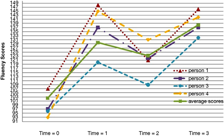
Figure 1. Four individual growth plots from four randomly selected participants and the average linear trajectory of all students across four time points.
This article demonstrates the use of TVCs to model discontinuous growth in a longitudinal dataset. A variety of other strategies exist to model non-linearities or discontinuities in the growth trajectory. Other shapes are accommodated easily using a variety of strategies. These include estimating piecewise models, polynomial models, or other non-linear models, as well as introducing TVCs (Singer and Willet, 2003 ).
Time-varying covariates are variables whose values can change across time. Although the value of the TVC changes across time, the parameter value estimating the effect of the TVC on the dependent variable is assumed to be constant across time. For example, in a study of vocabulary growth in children, the number of hours of TV that the child watches per week could be a TVC. At every time point, the researcher measures both the dependent variable (expressive vocabulary), and the independent variable (number of hours of TV the child watches per week). Although the number of hours of TV the child watches per week can change at each data collection point, the estimated relationship between TV viewing and vocabulary development remains constant across time. There are ways to ease this assumption. For example, one can build interaction between time and the TVC by creating a variable that equals the product of the two variables (Singer and Willet, 2003 ).
Illustration
The data for this demonstration (Reis, 2010 ) consist of reading fluency data measured on 277 elementary school students over four time points across two school years. The assessments were administered in the fall and spring of two consecutive school years. In addition, treatment also varied across time. Students were randomly assigned to either the treatment or the control group during year-1. During year-2, students were again randomly assigned to either the treatment group or the control group. Therefore, some students in the sample received the treatment during year-1 only, some students in the sample received treatment during year-2 only, some students received the treatment both years, and some students never received the treatment.
A preliminary inspection of the data revealed the non-linear nature of the average growth trajectory. Figure 1 plots four randomly selected students’ observed fluency scores across the four time points. In general, students’ observed reading fluency increased substantially from fall to spring of both school years. However, students’ observed fluency scores actually decreased between the spring of year-1 and the fall of year-2. Figures 2 –5 plot the actual and predicted fluency scores for all of the students in the sample across four time points, broken out by treatment group.
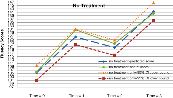
Figure 2. Actual and predicted growth trajectories for students who never received the treatment as well as 95% confidence intervals around the predicted growth trajectories.
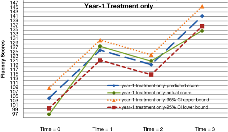
Figure 3. Actual and predicted growth trajectories for students who received the treatment during year-1 as well as 95% confidence intervals around the predicted growth trajectories.
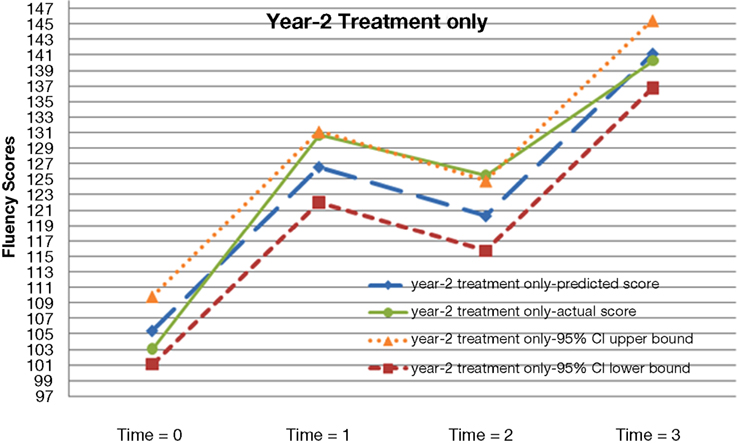
Figure 4. Actual and predicted growth trajectories for students who received the treatment during year-2 as well as 95% confidence intervals around the predicted growth trajectories.
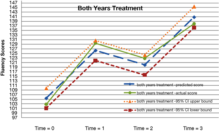
Figure 5. Actual and predicted growth trajectories for students who received the treatment during both years as well as 95% confidence intervals around the predicted growth trajectories.
Given the unusual shape of the growth trajectory, it was clear that a linear model was inappropriate. However, using a polynomial model would not solve our problem. A quadratic model would allow for a change in the rate of change. However, a quadratic model could only capture the shape of a growth trajectory with one bend. To capture the shape of this growth trajectory, which has two bends, would require a cubic model. The cubic model allows for a change in the change in the rate of change. In growth modeling, we can estimate t − 1 random effects, where t is the number of time points in the data set. Because there are four time points in this dataset, we can estimate three random effects. This allows us to estimate a random effect for the intercept, a random effect for the linear trajectory, and one other random effect. If we wanted to estimate a polynomial model, we could estimate a random effect for the quadratic term. However, we could not estimate a random effect for the cubic term. This means that we would have to assume that the cubic parameter was the same for every person in the sample, which seems an unlikely scenario. Thus, given that there were only four time points, estimating a cubic model seemed ill-advised.
Further, our goal was to simultaneously model the time-varying nature of the treatment and to capture the “summer slump effect” that was evident in the students’ growth trajectories. Thus, we needed to create a coding system that would capture the sharp discontinuity between the school years and the summer and would also allow us to model treatment as a TVC. To accomplish this, we created two sets of TVCs. The first set of TVCs was designed to capture the drop in fluency scores over the summer. The second set of TVCs was designed to model the treatment effect.
Modeling the Summer Slump
For the coding schemes that we present in this paper, we assume that students make the same amount of growth during each of the two school years. To do this, we constrained the growth from time 0 to time 1 and the growth from time 2 to time 3 to be equal 1 . Thus, we estimate one growth slope for both school years. However, we allow the growth rate from time 1 to time 2 (our summer slope) to differ from our school year slope. In this way, we are estimating a model that assumes linear growth during the school year, but allows for a completely different (and perhaps even negative) growth rate over the summer.
There are multiple ways to conceive of coding the over time data to capture the summer slump. First, one could view the trajectory in Figure 1 as a linear trajectory with a change in the intercept at time 2. This is the approach that we take in this paper. Therefore, we fit a linear growth trajectory across the four time points of data. To do this, we created a new variable, named time. This variable has four possible codes: 0, 1, 2, and 3. A code of time = 0 indicated that the data came from the first wave of data collection (in our case, fall of year-1); a code of time = 1 indicated that the data came from the second wave of data collection (in our case, spring of year-1), and so on. We also introduced a discontinuity at time 2 by fitting a change in the intercept. To do this, we created another new variable, a TVC called summer. This variable took on a value of 0 for all time points that occurred prior to the summer break (i.e., time point 1 (fall of year-1) and time point 2 (spring of year-2)). Summer was coded 1 for all time points that occurred after the summer break (i.e., time point 3 (fall of year-2) and time point 4 (spring of year-2)). Thus, the coding scheme for summer across the four waves of data collection was 0, 0, 1, 1. Table 1 , an excerpt from the data file, illustrates the coding for the time and summer variables. Using this coding scheme, the time variable captures a linear growth rate during the two school years, and the summer TVC captures the change in the growth rate that occurs during the summer months. Therefore, to obtain the actual summer growth rate, one simply adds the parameter estimate for the linear growth rate (β10) to the parameter estimate for the change in intercept over the summer (β20).
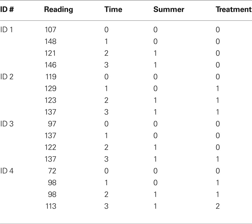
Table 1. An excerpt of the data file for four sample students.
Alternately, one could model two separate slopes, a school year slope and a summer slope. In such a scenario, the school year slope would be coded 0, 1, 1, 2 and the summer slope would be coded 0, 0, 1, 1. In either of these coding systems, the TVC that captures the summer slope is coded the same way. What differs is the treatment of the original time variable. However, because the coding of the time variable changes across the two systems, both the parameter estimate for and the interpretation of the TVC also change. When time is coded 0, 1, 2, 3, and the summer slump variable is coded 0, 0, 1, 1, then the summer slump variable represents the amount by which the linear growth slope must be adjusted downward to capture the discontinuity in the trajectory. If the first time variable is coded 0, 1, 1, 2 and the summer slope is coded 0, 0, 1, 1, then the first time variable (β10) represents the linear growth during the school year and the summer TVC (β20) represents the summer growth slope.
We also coded the intervention variable as a TVC. As mentioned earlier, students could be in one of four possible groups: those who received the intervention during year-1, those who received the intervention during year-2, those who received the intervention both years, and those who did not receive the intervention either year. Our modeling of the treatment effect needed to meet certain criteria. First, the students who received treatment both years received twice as much treatment as those who received treatment during year-1 only or year-2 only. Second, no one received any treatment between the spring of year-1 (time point 2) and the fall of year-2 (time point 3). Therefore, theoretically, the growth during that time period should be unaffected by the student’s intervention group. Third, because students were randomly assigned to treatment, the treatment group should not have an impact on students’ initial scores. Ideally, students from the various groups should have similar values on the intercept. However, even if the groups differed in terms of their intercepts, those differences could not be attributed to receipt of the treatment because the first time point of data collection occurred prior to the start of the intervention. Finally, we wanted to model a treatment effect that persisted over time, so that any effects attributed to the treatment would be maintained even after the treatment was completed. However, we did not want the treatment effect to continue to impact the growth slope after the treatment was complete. In other words, any reading gains that students made as a result of the treatment should persist over time; however, we would not expect the growth slope of the treatment group to be steeper than the growth of the non-treatment group during non-instructional months. To capture this process, we created a TVC for treatment. The coding scheme this treatment variable is depicted in Table 1 . Because the treatment did not begin until after the first wave of data collection, all students received a 0 during the first wave of data collection. Then, a student’s score on the treatment variable increased by 1 for each time point during which he or she received the treatment. Therefore, a student who was in the control group during both years of data collection received a score of 0 at each time point (0, 0, 0, 0). A student who was in the treatment group for year-1 received a score of 0,1,1,1. This allowed the growth rate from time 1 to time 2 to be impacted by the treatment. Coding the third and fourth time points as 1’s allowed the effects of the treatment to persist, undiminished over time. However, this coding system did not allow the differential growth rate that occurred between time points 1 and 2 to continue after the end of the intervention. A student who was in the treatment group during year-2 was coded 0, 0, 0, 1. Finally, a student who was in the treatment group during both years of the study was coded as 0, 1, 1, 2. Table 1 , which contains an excerpt of the data file, illustrates this coding scheme.
One could make different assumptions about the effect of the intervention across time, and these assumptions would obviously affect the coding system. For example, one might expect the intervention to permanently impact the slope of the growth trajectory. In such a scenario, once a student received the intervention, their growth trajectory would be permanently deflected. For example, perhaps certain reading strategy interventions might teach students how to become better readers. Perhaps after receiving intervention, the student is able to grow more quickly in terms of his or her reading skills, and he/she is able to maintain this differential growth, even after the intervention is complete. If a researcher believes that the growth trajectory of the dependent variable is permanently altered by the introduction of the treatment, then such an effect could be captured by introducing a second time variable that “turns on” when the treatment begins and continues to “tick” throughout the remainder of data collection. In contrast, one might expect that any effects of the intervention are fleeting and diminish or disappear once the intervention ceases. Behavioral interventions may follow such a pattern. One might see growth in a client’s social skills or positive behaviors when he or she is receiving positive reinforcement. However, when the reinforcers are withdrawn, the client may return to baseline. In such a scenario, there are no lasting impacts of treatment once the intervention is withdrawn: the intervention effect is fleeting, rather than permanent. To capture the fleeting nature of the intervention, one could introduce a TVC that allows for a change in slope during the intervention period but then goes back to baseline (0) after the intervention is withdrawn. Table 2 contains the coding schemes for summer, persistent treatment effects, and fleeting treatment effects.
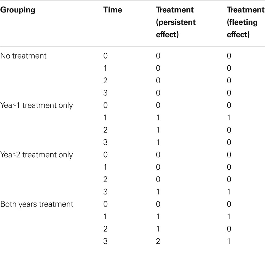
Table 2. Coding schemes.
Analysis
To examine the differences in the growth in reading fluency across instructional groups at two elementary schools (Jupiter and Keeney), we estimated a series of multilevel models using HLM version 6.4 (Raudenbush et al., 2004 ). Our dependent variable was mean oral reading fluency (ORF). Measures of ORF assess the speed, accuracy, and efficiency with which a student reads a particular text. All s tudents read from three increasingly difficult, 250-word passages for three separate 1-min reading trials. Interventionists recorded the number of words read correctly for each passage and calculated a mean ORF score for each student. The overall mean on ORF was 123.30 with a standard deviation of 29.29. Scores ranged from a low of 9 to a high of 245.
As mentioned previously, this study included 2 years of longitudinal reading intervention program data. Some students received treatment during only year-1; some students received treatment during only year-2; some students received treatment during both in year-1 and year-2, and some students never received the treatment. Table 1 contains coding scheme that we used in our analyses. Table 3 contains the descriptive statistics for this example.
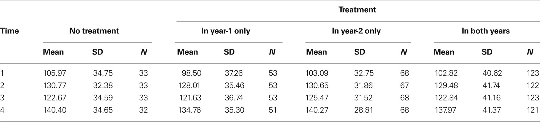
Table 3. Descriptive statistics – two schools combined.
We hypothesized that (1) modeling summer as an additional TVC would allow us to more accurately capture the shape of the students’ growth trajectories, (2) the addition of treatment as a TVC would allow us to explore the effect of treatment on reading fluency. If the treatment did have an effect on reading fluency, then the addition of the treatment TVC should help to explain within-person change over time more precisely.
Model-1: The Unconditional Linear Growth Model
The first level-1 growth model (model-1) was a simple linear growth model. It contained a linear growth slope (coded 0, 1, 2, 3) but did not model the treatment effect or the summer effect. The model for the unconditional linear growth model was:
Yij = π0i + π1i(time) + eit
π0i = β00 + r0i
π1i = β10 + r1i
At Time = 0 in the fall of year-1, the average fluency score was 108.17. In addition, mean reading fluency increased at a rate of 10.05 per wave. There was statistically significant variation in the intercept across all students in the population (τ00 = 1258.79, χ2(276) = 2956.2, p < 0.001). This suggested there was variability in terms of students’ initial reading fluency scores. The chi-square test of the variance components (i.e., τ00, τ11 presented in this paper) are described in Raudenbush and Bryk (2002 , pp. 63–64). We use these statistical tests, in combination with the chi-square difference test (comparing the deviances of two different models) to determine whether or not to include a random effect in the model. We do not rely on the Wald test, which is reported in statistical packages such as SPSS and SAS because using the Wald test to determine the statistical significance of variance components is known to be inaccurate (Raudenbush and Bryk, 2002 ).
Model-2a: Linear Growth with Summer as a Time-Varying Covariate
In model-2a, we added the summer slope as TVC. We added an additional time-varying covariate that accounted for the non-instructional period between time 1 and time 2. Again, this variable was coded 0, 0, 1, 1, and time was coded 0, 1, 2, 3. Therefore, the summer slope captured the differential between the school year growth rate and the summer growth rate. In other words, the coefficient for this slope (β20) represents change in the intercept between time points 1 and 2, and β20 indicated how much less (or more) growth we expect the student to make over that non-instructional period.
We needed to decide whether to estimate the summer slope as fixed or randomly varying. If we fixed the summer slope, then every student in the sample would have the same estimate of summer gain/loss. If we allowed the summer slope to randomly vary, then we would estimate a mean summer slope and a residual for each person in the sample. Therefore, the summer effect could take on a different value for every person in the sample. At first blush, allowing the slope of the summer effect to randomly vary across people might seem preferable to fixing the slope. However, Raudenbush and Bryk (2002) caution against estimating all slopes as randomly varying by default. Instead, the goal is to build the most parsimonious model that provides a reasonable fit to the data. Raudenbush and Bryk warn that “if one overfits the model by specifying too many random level-1 coefficients, the variation is partitioned into many little pieces, none of which is of much significance” (p. 256). Therefore, we ran the model both with and without the random effect for summer and compared the fit of the model. When we included the random effect for the summer slope, the variance of the summer slope was not statistically different from 0 (χ2(275) = 7.14, p > 0.50). In addition, including the three additional variance–covariance components to the model only decreased deviance by 0.80 points. The chi-square difference test (χ2(3) = 0.80) favored the model with the fixed summer slope. Therefore, the final model that we present here and in Table 5 is the model with a fixed summer slope. We describe the logic of the chi-square difference test and other model fit criteria in more detail later in the paper, in the section on statistical approaches for evaluating the adequacy of the level-1 model.
The final equations for model-2a are below.
Yij = π0i + π1i(time) + π2i(summer) + eij
π0i = β00 + r0i
π1i = β10 + r1i
π2i = β20
For model-2a, in the fall of year-1, the average fluency score was 105.45. In addition, mean reading fluency increased at a rate of 20.93 points during the school year. Also, the average effect of summer was statistically significant (β20 = −27.23, p < 0.001). This means that whereas students were growing an average of almost 21 points per wave during the school year in terms of their reading fluency, they were actually losing about 6.3 points (20.93–27.23) over the summer.
Adding summer as a TVC explained an additional 36.43% of the within-person variation in reading fluency (over and above the linear growth model), suggesting that there was much less error in the prediction of students’ level-1 growth trajectories once we added the TVC to capture the summer slump.
Model-2b: Linear Growth with Treatment as a Time-Varying Covariate
In model-2b, we added treatment as TVC. Remember that treatment captures whether students were exposed to the treatment on varying time points across the study. Table 1 provides the coding system for the time-varying treatment variable. For pedagogical purposes, we did not include the summer TVC in model-2b so that we could illustrate the problems that can occur when the level-1 growth trajectory is not properly modeled. Again, we ran the model two ways. First, we allowed the slope of the treatment variable to randomly vary across people. Next, we fixed the slope of the treatment effect. The variance of the treatment slope was not statistically significantly different from 0 (χ2(242) = 249.6, p = 0.36) and the chi-square difference test for the difference in deviances between the two models was not statistically significant (χ2(3) = 1.35). Therefore, the final model presented here and in Table 5 is the model with the fixed treatment effect slope.
Yij = π0i + π1i(time) + π2i(treatment) + eit
π0i = β00 + r0i
π1i = β10 + r1i
π2i = β20
For model-2b, in the fall of year-1, the average fluency score was 107.74. In model-2b, the intercept for the reading fluency growth slope (β10) was 6.76. In other words, the predicted reading fluency increased at a rate of 6.76 per semester for students who were never exposed to the treatment (students who were coded 0, 0, 0, 0 on the time-varying treatment variable). This is very different from the mean growth rate in model-2a, which predicted 20.93 points of reading growth during the school year and 6.3 points of reading loss over the summer. There are two possible reasons for this difference. First, β10 represents the predicted growth slope for students who never received the treatment, not the overall predicted growth slope. Second, the summer slope is not included in the model.
In this model, the average effect of treatment was statistically significant (β20 = 8.26, p < 0.001). However, this was a naïve analysis which assumed linear growth rate during both instructional and non-instructional periods. When we plotted the average scores in each condition across each time point using the descriptive statistics from the sample, we could clearly see that the growth trajectory was not linear over the time. Thus Model-2b was misspecified; it failed to account for the differential growth of students during the non-instructional months (summer). Fluency scores decreased during the summer, yet model-2b failed to capture thus discontinuity. Although model-2b suggested that the treatment effect was statistically significant, this finding was estimated using an inappropriate level-1 model. Therefore, these results cannot be trusted.
When comparing model-2b to model-1, adding treatment as an additional TVC only explained an additional 2.75% of the within-person variation in reading fluency.
Model-3: Modeling Summer Slump and Treatment as Time-Varying Covariates
In model-3, we combined model-2a and model-2b. Thus, we simultaneously modeled two TVCs: treatment and the summer slope. Table 1 provides the coding scheme for both TVCs. Because neither of the slopes for the TVCs needed to randomly vary in models 2a and models 2b, we fixed the slopes for both TVCs in model-3. The equations for model-3 appear below.
Yij = π0i + π1i(time) + π2i(summer) + π3i(treatment) + eit
π0i = β00 + r0i
π1i = β10 + r1i
π2i = β20
π3i = β30
In model-3, the intercept (β00 = 105.45, p < 0.001) represents the average fluency of students at the beginning of the study. In addition, holding treatment constant at 0, mean reading fluency increased at a rate of 21.10 per semester (β10 = 21.10, p < 0.001). After controlling for treatment, the average effect of summer was −27.39 and it was statistically significant from zero (β20 = −27.39, p < 0.001). Therefore, a non-treatment student’s predicted score in the spring of year-1 was 105.45 + 21.10, or 126.55. A non-treatment student’s predicted score for fall of year-2 was 105.45 + 2(21.10) + (−27.39), or 120.26. Further, we predicted that the average student experiences 6.29 (21.10 + (−27.39)) points of summer fluency loss between spring of year-1 and fall of year-2. In other words, regardless of the treatment group, the predicted ORF score for a student in the fall of year-2 was 6.29 points lower than the predicted score for spring of year-1. This is because the negative change in intercept (β20 = −27.39) outweighs the constant linear slope effect (β10 = 21.10) that we were modeling across the four time points of data collection. This drop represents a “summer slump,” where students’ ORF scores actually decreased during the non-instructional months. The effect of treatment (β30 = −0.25, p = 0.84), our TVC, was not statistically significantly different from zero, indicating the treatment failed to impact students’ growth in ORF scores. Once we included the summer slope as a TVC, the effect of treatment was no longer statistically significant. Therefore, misspecifying the shape of the level-1 model could have led us to conclude that the treatment was effective when in fact, it was not.
The results from final level-1 model (model-3) suggested that we were able to reduce the within-person residual variance by 36.4% over the linear model (model-1) by introducing our two TVCs (summer and treatment). Furthermore, the final level-1 model (model-3) reduced the within-person residual variance by 30.8% over the linear model with treatment (model-2b) by introducing our summer as TVC. Most importantly, model-4 more correctly captured the shape of our growth trajectory than model-2b did.
In an effort to visualize the meaning of these parameters, we calculated the predicted scores for each time point. We then graphed these scores and compared them to the mean actual scores. These predicted scores are reported in Table 4 and Figures 2 –5 .
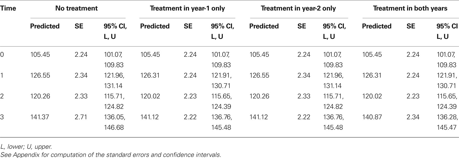
Table 4. Predicted scores, standard errors, and 95% confidence intervals for the predicted scores.
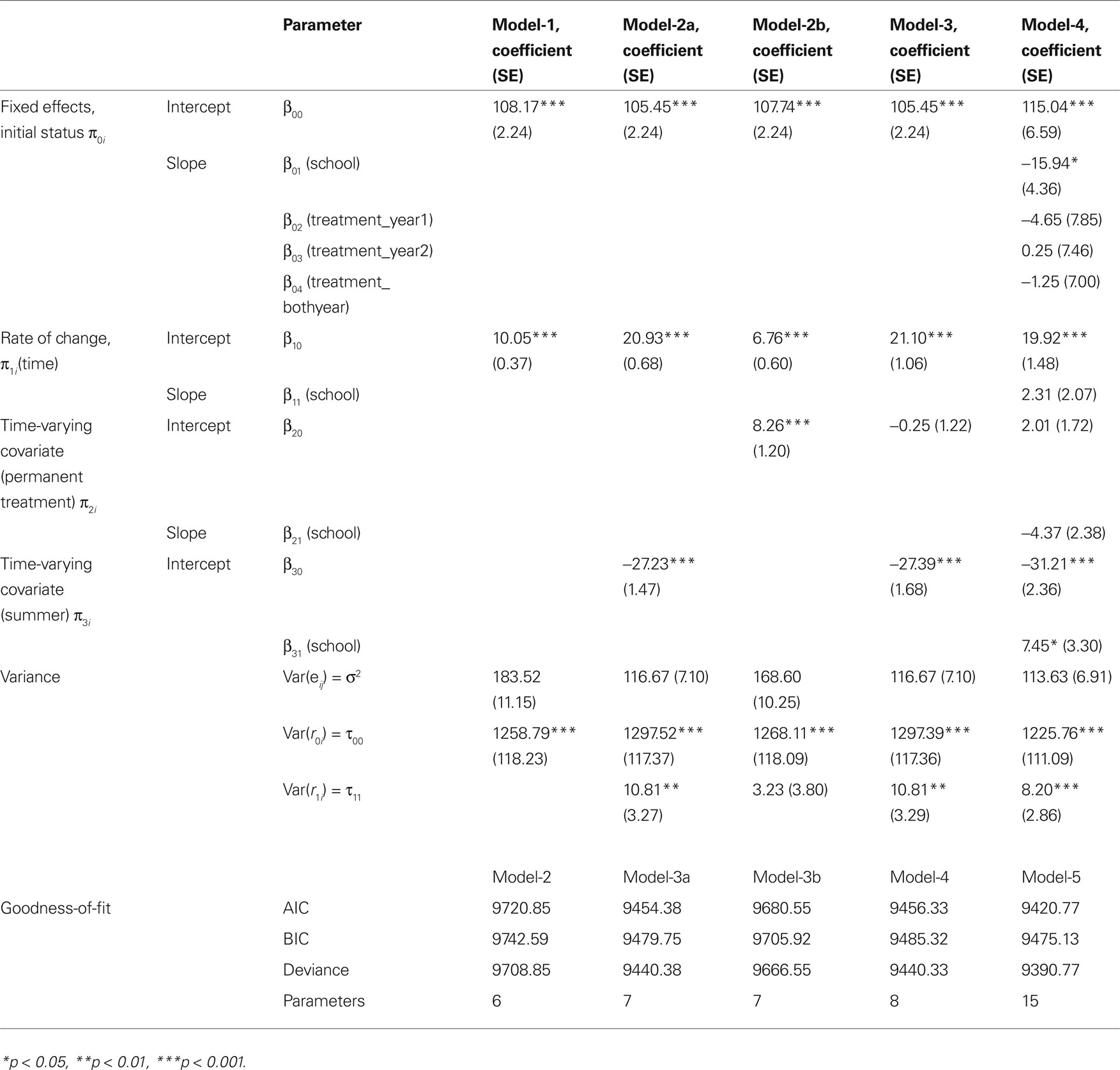
Table 5. Parameter estimates for the five growth models.
Level-2 Model
To examine between-person variability in reading fluency, we introduced several level-2 predictors. We added a dummy coded variable representing school (coded as 0 = Keeney and 1 = Jupiter) as a predictor of both the intercept and all three slopes. We also added treatment as a time invariant predictor of the intercept. Since there were four levels of treatment, we created three dummy coded variables: treatment only during year-1; treatment only during year-2 and treatment in both years. Thus the reference group consisted of students who did not receive any treatment. Adding treatment as a time invariant predictor of the intercept allowed us to test for and model baseline differences among the treatment groups. However, it would not make sense to add treatment as a time invariant predictor of the growth slopes because treatment was already added to the model as a TVC (β20). The equations for model-4, the full 2-level model, appear below.
Yij = π0i + π1i(time) + π2i(summer) + π3i(treatment) + eij
π0i = β00 + β01(school) + β02(TRT_yr1) + β03(TRT_yr2) + β04(TRT_bothyr) + r0i
π1i = β10 + β11(school) + r1i
π2i = β20 + β21(school)
π3i = β30 + β31(school)
In the full level-2 model, the intercept (β00 = 115.04, p < 0.001) represents the mean initial reading fluency score for students who never received the treatment and who attended Keeney. The coefficient for effect of the school on the intercept (β01 = −15.94, p = 0.001) represents the differential in the initial average reading fluency score between students attending Keeney and Jupiter. In other words, the students at Jupiter scored 15.94 points lower on initial reading fluency than their peers at Keeney; therefore, the predicted initial reading fluency score for a student who attended Keeney and who was never exposed to the treatment was 99.10 (115.04 − 15.94). The differential between students who were exposed to treatment only during year-1 and those who never exposed to treatment on the initial reading fluency score (β02) was −4.65. After controlling for school, students who never exposed to treatment scored 4.65 points higher on initial reading fluency than their peers who were exposed to treatment during only year-1; however, this difference was not statistically significantly different from zero (β02 = −4.65. p = 0.53). After controlling for school, the predicted reading fluency scores for those students who never exposed to treatment were 0.25 points lower than their peers who were exposed to treatment during only year-2; again, this difference was not statistically significantly different from zero (β03 = 0.25, p = 0.97). Lastly, after controlling for school, students who never exposed to treatment had ORF scores that were 1.25 points higher than their peers who were exposed to treatment in both years; however, again, this differential was not statistically significantly different from zero(β04 = −1.25, p = 0.86).
The results suggested that the mean initial reading fluency score increased at a rate of 19.92 points per semester (β10 = 19.92, p < 0.001) for students attending at Keeney when the effect of the treatment was held constant. Although school was statistically significant predictor of students’ initial reading fluency, it did not predict the linear rate of growth in students’ reading fluency (β11 = −2.31, p = 0.27). Again, the effect of the summer slope on reading fluency was statistically significantly different from zero (β20 = −31.21, p < 0.001). In other words, Keeney (the reference school) students’ scores increased by 19.92 points between fall and spring of year-1, then they decreased by 11.29 points between spring of year-1 and fall of year-2. This is because the change from time 2 to time 3 would be 19.92 + (−31.21), or −11.29. Thus when both treatment and summer effects were taken into account simultaneously, right after summer, the reading scores of students attending at Keeney who never exposed to treatment were 11.29 points lower than they had been before the summer. At Jupiter, the effect of the summer slope on reading fluency was −23.76 (−31.21 + 7.45), indicating that the summer slump parameter was 7.45 points less pronounced at Jupiter (β21 = 7.45, p = 0.024). At Jupiter, students who were never exposed to treatment had predicted reading fluency scores after summer break were 1.53 points lower than their spring scores (−31.21 + 7.45 + 19.92 + 2.31). The average effect of the treatment on reading fluency at Keeney was not statistically significantly different from zero nor did the effect of the treatment did differ by school (β31 = −4.37, p = 0.07). Thus, in this particular example, treatment had no effect on reading fluency scores.
Assessing the Adequacy of the Level-1 Model
Again, we cannot overemphasize the importance of correctly modeling the shape of the growth trajectory. To determine whether we were adequately capturing the shape of the growth trajectory with our level-1 model, we relied on a combination of graphical and statistical approaches.
Graphical Approaches
First, we plotted the average growth across the four time points of data collection using our sample statistics and we compared the shape of that trajectory to the shape of the trajectory produced by our model predicted values. If we have adequately captured the form of the level-1 model, the shape of the model predicted growth trajectory should strongly resemble the shape of the growth trajectory using actual data. We can also compare the model predicted scores to the actual scores using our sample data. Although the model predicted scores would not match the actual scores exactly, the model predicted scores and the actual scores should approximate each other. If the model predicted scores are drastically different from the actual scores, this may suggest a misspecification of the level-1 model.
To aid in our graphical analyses, we computed the 95% confidence intervals for the predicted scores for each of the treatment groups and compared them to the actual mean scores for each of the groups. Ideally, the actual scores should fall within the 95% confidence intervals approximately 95% of the time. In our example, 14 of the 16 datapoints (87.5%) fell within the 95% confidence intervals for the predicted scores. The Appendix of this document illustrates the computation of these 95% confidence intervals.
In this paper, we have plotted the average predicted trajectory and the average actual trajectory. However, researchers should also examine the individual empirical growth plots and compare them to the ordinary least square estimated individual trajectories (Singer and Willet, 2003 ). The comparison of these plots should provide additional evidence that the model has adequately captured the shape of the level-1 growth trajectory.
Statistical Approaches
We can also compare the deviances and model fit indices such as the AIC and BIC for a variety of level-1 models. These model comparisons allow us to make inferences about which models appear to provide the best fit. Multilevel modeling uses maximum likelihood (ML) techniques to produce estimates of the model parameters. The likelihood function captures “the probability of observing the sample data as a function of the model’s unknown parameters” (Singer and Willet, 2003 , p. 66). Using ML to estimate the parameters of the model also provides this likelihood, which is then transformed into a deviance statistic (Snijders and Bosker, 1999 ).
The deviance compares the log-likelihood of the specified model to the log-likelihood of a saturated model that fits the sample data perfectly (Singer and Willet, 2003 , p. 117). Specifically, deviance = −2 (log-likelihood of the current model − log-likelihood of the saturated model) (−2LL) (Singer and Willet). Therefore, deviance is a measure of the badness of fit of a given model; it describes how much worse the specified model is than the best possible model (Singer and Willet). Deviance statistics cannot be interpreted directly since deviance is a function of sample size as well as the fit of the model. However, for models that are hierarchically nested and use the same sample, researchers can compute and interpret differences in deviance for competing models estimated using full maximum likelihood estimation (FIML) (McCoach and Black, 2008 ). Hierarchically nested models that differ only in terms of their random effects can be compared using deviances derived from restricted maximum likelihood estimation (REML). However, if two hierarchically nested models differ in terms of their fixed effects, we must use deviances obtained using FIML to make any model comparisons.
If two models are nested and the model is estimated using FIML, the deviance statistics of two models can be compared directly. The deviance of the simpler model (Ds) minus the deviance of the more complex model (Dc) provides the change in deviance (ΔD = Ds − Dc). The deviance of the more complex model must be lower than (or as low as) that of the simpler model. In large samples, the difference between the deviances of two hierarchically nested models is distributed as an approximate chi-square distribution with degrees of freedom equal to the difference in the number of parameters being estimated between the two models (de Leeuw, 2004 ).
To decide among competing level-1 models, we can compare two hierarchically nested models using the chi-square difference test. The chi-square difference test helps us determine whether the additional parameterizations using TVCs help to improve the fit of the model. In our current analysis, we can compare the fit of the linear growth model that includes a TVC for treatment (model-2b) to the model that includes a discontinuity for the summer period as well as a TVC for treatment (model-3). The deviance for model-2b (the simpler model) is 9666.55 with seven parameters. The deviance for model-3 (the more parameterized model) is 9440.33 with eight parameters. Thus, the deviance drops by 226.22 with the addition of one parameter, the summer slope parameter. This large decrease in the deviance indicates that adding the summer slope parameter does indeed improve the fit of the model.
The Akaike information criterion
The formula for the Akaike information criterion (AIC) is shown below.

where D is deviance and p = the number of parameters estimated in the model.
To compute the AIC, simply multiply the number of parameters by two and add this product to the deviance statistic, computed using FIML. The addition of 2p to the deviance statistic imposes a small penalty based on the complexity of the model. When there are several competing models, the model with the lowest AIC value is considered to be the best model. An advantage of the AIC is that it can be used to compare non-hierarchically nested models. In our current example, we can use the AIC to compare the fit of model-2a to that of model-2b. The AIC for model-2a is 9440.38 + 2 × 7 = 9454.38. The AIC for model-3b is 9666.55 + 2 × 7 = 9680.55. Model-2a (the model with the summer slope) has a smaller AIC than model-2b (the model with the treatment TVC); therefore, we would favor model-2a over model-2b.
The Bayesian information criterion (BIC)
The Bayesian information criterion (BIC) is equal to the sum of the deviance and the product of the natural log of the sample size and the number of parameters. The formula for the BIC is shown below.

where D is deviance (−2LL),
p = the number of parameters estimated in the model, and
n = the sample size.
Therefore, the BIC imposes a penalty on the number of parameters that is impacted directly by the sample size. For these analyses, we use the number of people (or level-2 units) as our sample size. To illustrate the BIC, we compare models-3a and 4. The BIC for model-3a is 9440.38 + 7 × ln(277) or 9479.75. The BIC for model-4 is 9440.33 + 8 × ln(277) or 9485.32. Thus, using the BIC, we would favor model-2a over model-3. All three of the model fit tests we have outlined (the chi-square difference, the AIC, and the BIC) favor model-2a over model-3. This is because the extra parameter that we introduce in model-3 only decreases the deviance by 0.05 over the deviance in model-2a. These results suggest that adding treatment as a TVC does not improve the fit of the model that includes the summer slope. This should not be surprising, given that treatment was not a statistically significant predictor of ORF.
Finally, an examination of the residual terms can prove valuable in determining the aptness of the level-1 model. Most programs can produce files that contain the residuals for all level-1 observations (eti) and the residuals for all level-2 observations (r0i, r1i, etc.). Checking for the normality of the distribution of level-1 and level-2 residuals using exploratory analyses and P–P plots provides additional information about the adequacy of the model (Singer and Willet, 2003 ). For more information on residual analyses, see Singer and Willet (2003 , pp. 128–132).
Intervention Effect
In part, the modeling of the intervention effect depends upon the assumptions that the analyst makes about the persistence of the intervention effect. In our analyses, we modeled an effect which persisted over time, but which did not have a lasting impact on the growth slope. We call this a persistent effect. There are two other possible ways to conceive of an intervention effect. One could conceive of an intervention effect that deteriorates or dissipates over time. In our example, one might hypothesize that any intervention effects would decay over the summer vacation. We call this a fleeting effect. Table 2 contains a coding scheme that captures a fleeting treatment effect, as well as the coding scheme for a persistent treatment effect. Notice that the most important difference between the fleeting and the persistent treatment effects really occurs between times 2 and 3. While the treatment effect “disappears” under the fleeting coding scheme, any advantage that the treatment group accrues is maintained under the permanent coding scheme. It is possible to fit both of these models to the data and compare the coding schemes to each other to determine which coding system appears to better fit the data. In our example, because the intervention effect was not statistically significant, comparing these two models would not provide any additional information about the nature of the intervention effect. In reality, it is possible that a treatment effect is neither completely maintained, nor does it completely deteriorate over the summer break. If one knew the degree of decay a priori, this could be built into the coding scheme. For example, if one knew that only 50% of the treatment effect were maintained across the summer break, one could code the treatment effect as 0, 1, 0.5, 1.5 for a student who received treatment during both years of the study.
In conclusion, the multilevel model for change provides a flexible way to model a variety of growth trajectories and to incorporate time-varying variables into the analysis. In growth curve modeling, capturing the shape of the level-1 growth trajectory is essential: misspecifications of the level-1 model can lead to errors of inference in both the level-1 and level-2 models. Incorporating TVCs provides one method of modeling non-linearities or discontinuities in growth trajectories. There are a variety of strategies for coding TVCs; we have illustrated just a couple of basic coding schemes. Correct and creative coding of time-varying variables can help to more adequately capture the nature of the change in the phenomenon of interest. We hope that our simple illustration serves to alert analysts to the dangers of conducting sophisticated statistical modeling without adequately understanding the nature and the shape of the data at hand.
Appendix
Computation of the Standard Errors Of the Predicted Scores
To construct the 95% confidence interval of the predicted score, one needs not only the predicted scores but also the standard error of the predicted scores. Therefore, we calculated the variation of the predicted score by using covariance algebra in an effort to find the standard error of the predicted score. Our final level-1 model (model-4) is
yij = β00 + r0i + (β10 × wave) + (r1i × wave) + β20(summer) + β30(treatment) + eij
The variance of the predicted score  can be calculated from the following equation:
Accordingly, we need the variance–covariance matrix of the fixed effect parameter estimates. HLM program (Raudenbush et al., 2004
) provides this matrix when it is asked as output option. When the parameter estimates of variances and covariances were inserted into the Eq. A1, we were able to calculate the variance of the predicted score of  For example, based on our coding scheme demonstrated in Table 1
, the variance of predicted score of student who was in the year-1 treatment only group at time = 1 is
For example, based on our coding scheme demonstrated in Table 1
, the variance of predicted score of student who was in the year-1 treatment only group at time = 1 is
When the variances/covariances of estimates were integrated into the above equation, we calculated the variance of the predicted score where the square root of this term is equal to its standard error.
Conflict of Interest Statement
The authors declare that the research was conducted in the absence of any commercial or financial relationships that could be construed as a potential conflict of interest.
Footnote
- ^ To be consistent with the literature on growth modeling, we refer to the initial time point as time 0 throughout the paper. Thus our four waves of data collection are referred to as time 0, time 1, time 2, and time 3.
References
Bollen, K. A., and Curran, P. J. (2006). Latent Curve Models: A Structural Equation Perspective. Hoboken, NJ: Wiley.
de Leeuw, J. (2004). Multilevel analysis: techniques and applications (Book review). J. Educ. Meas. 41, 73–77.
McCoach, D. B. and Black, A. C. (2008). “Assessing model adequacy,” in Multilevel Modeling of Educational Data, eds A. A. O’Connell and D. B. McCoach (Charlotte, NC: Information Age Publishing), 245–272.
Raudenbush, S., Bryk, A., Cheong, Y. F., Congdon, R., and du Toit, M. (2004). HLM6: Hierarchical Linear and Non-Linear Modeling. Lincolnwood, IL: Scientific Software International.
Reis, S. M. (2010). Using the Schoolwide Enrichment Model Reading Framework (SEM-R) to increase achievement, fluency, and enjoyment in reading. Jacob K. Javits grant funded by the United States Department of Education, Office of Secondary and Elementary Programs
Singer, J. D., and Willet, J. B. (2003). Applied Longitudinal Data Analysis: Modeling Change and Event Occurrence. New York: Oxford.
Keywords: hierarchical linear modeling, multilevel modeling, growth curve modeling/growth curve model(s), time varying covariates, coding, summer effects, time varying treatment effects
Citation: McCoach DB and Kaniskan B (2010) Using time-varying covariates in multilevel growth models. Front. Psychology 1:17. doi: 10.3389/fpsyg.2010.00017
This article was submitted to Frontiers in Quantitative Psychology and Measurement, a specialty of Frontiers in Psychology
Received: 19 February 2010;
Paper pending published: 10 March 2010;
Accepted: 18 May 2010;
Published online: 14 June 2010
Edited by:
Jeremy Miles, Research and Development Corporation, USAReviewed by:
Gary Adamson, University of Ulster, UKDavid Flora, York University, Canada
Copyright: © 2010 McCoach and Kaniskan. This is an open-access article subject to an exclusive license agreement between the authors and the Frontiers Research Foundation, which permits unrestricted use, distribution, and reproduction in any medium, provided the original authors and source are credited.
*Correspondence: D. Betsy McCoach, Measurement, Evaluation, and Assessment Program, Educational Psychology Department, Neag School of Education, University of Connecticut, 249 Glenbrook Road, Unit 2064 Storrs, CT 06269-2064, USA. e-mail: betsy.mccoach@uconn.edu