Testing Transitivity of Preferences on Two-Alternative Forced Choice Data

Regenwetter, Michel; Dana, Jason; Davis-Stober, Clintin P.

doi:10.3389/fpsyg.2010.00148

PERSPECTIVE article

Front. Psychol., 13 December 2010

Sec. Quantitative Psychology and Measurement

Volume 1 - 2010 | https://doi.org/10.3389/fpsyg.2010.00148

Testing Transitivity of Preferences on Two-Alternative Forced Choice Data

Michel Regenwetter¹*

Jason Dana²

Clintin P. Davis-Stober³

¹ Department of Psychology, University of Illinois at Urbana-Champaign, Champaign, IL, USA
² Department of Psychology, University of Pennsylvania, Philadelphia, PA, USA
³ Department of Psychological Sciences, University of Missouri, Columbia, MO, USA

As Duncan Luce and other prominent scholars have pointed out on several occasions, testing algebraic models against empirical data raises difficult conceptual, mathematical, and statistical challenges. Empirical data often result from statistical sampling processes, whereas algebraic theories are nonprobabilistic. Many probabilistic specifications lead to statistical boundary problems and are subject to nontrivial order constrained statistical inference. The present paper discusses Luce’s challenge for a particularly prominent axiom: Transitivity. The axiom of transitivity is a central component in many algebraic theories of preference and choice. We offer the currently most complete solution to the challenge in the case of transitivity of binary preference on the theory side and two-alternative forced choice on the empirical side, explicitly for up to five, and implicitly for up to seven, choice alternatives. We also discuss the relationship between our proposed solution and weak stochastic transitivity. We recommend to abandon the latter as a model of transitive individual preferences.

Introduction

For algebraic axioms and relevant empirical data resulting from a random sampling process, it is necessary to bridge the conceptual and mathematical gap between theory and data. This problem has long been known as a major obstacle to meaningful empirical axiom testing (e.g. Luce, 1995, 1997). Luce’s challenge is to (1) recast a deterministic axiom as a probabilistic model, or as a suitable hypothesis, with respect to the given empirical sample space and (2) use the appropriate statistical methodology for testing the probabilistic model of the axiom, or the corresponding hypothesis, on available behavioral data.

We concentrate on the axiom of transitivity, a pivotal property of “preference” relations. Transitivity is shared by a broad range of normative as well as descriptive theories of decision making, including essentially all theories that rely on a numerical construct of “utility.” The literature on intransitivity of preferences has not successfully solved Luce’s challenge in the past (see also Regenwetter et al., 2011). We concentrate on the dominant empirical paradigm, two-alternative forced choice, which forces two additional axioms to hold on the level of the empirical binary choices. Jointly with transitivity, these two axioms model preferences as strict linear orders. We discuss what we consider the first complete solution to Luce’s challenge for (transitive) linear order preferences and two-alternative forced choice data for currently up to seven choice alternatives. We explicitly provide the complete solution for up to five choice alternatives. We endorse and test a model which states that binary choice probabilities are marginal probabilities of a hypothetical latent probability distribution over linear orders.

After we introduce notation and definitions, we explain why most of the literature has not successfully solved Luce’s first challenge of formulating an appropriate probabilistic model of transitive preferences. Then, we proceed to introduce the mixture model of transitive preference that we endorse. Next, we review Luce’s second challenge and how it can be overcome in the case of the mixture model.

Notation and Definitions

Definition. A binary relation B on a set 𝒞 is a collection of ordered pairs B ⊆ 𝒞 × 𝒞. For binary relations B and R on 𝒞, let BR = {(x,z) | ∃y ∈ 𝒞 with (x,y) ∈ B,(y,z) ∈ R}. A binary relation B on 𝒞 satisfies the axiom of transitivity if and only if

A binary relation is intransitive if it is not transitive.

At various places in the manuscript, we will use other properties of binary relations as well. We define these next.

Definition. Let 𝒞 be a finite collection of choice alternatives. Let I_𝒞 = {(x,x) x ∈ 𝒞 }. Given a binary relation B, we write B⁻¹ = {(y,x) | (x,y)∈B} for its reverse and yes for its complement. A binary relation B on 𝒞 is reflexive if I_𝒞 ⊆ B, strongly complete if B ∪ B⁻¹ ∪ I = 𝒞 × 𝒞, negatively transitive if yes asymmetric if yes A weak order is a transitive, reflexive and strongly complete binary relation, and a strict weak order is an asymmetric and negatively transitive binary relation.

We assume throughout that 𝒞 is a finite set of choice alternatives. In models of preference, it is natural to write (x,y) ∈ B as xBy and to read the relationship as “x is preferred to (better than) y”. (For additional definitions and classical theoretical work on binary preference representations, see, e.g. Luce, 1956; Fishburn, 1970, 1979, 1985; Krantz et al., 1971; Roberts, 1979).

The Empirical Sample Space in Empirical Studies of Transitivity

To formulate a probabilistic model concisely, it is critical first to understand the sample space of possible empirical observations. Once that sample space is specified, one can formulate any probabilistic model as a mapping from a suitably chosen parameter space (here, this is a probability space that models latent preferences) into that sample space. The more restrictive the parameter space and its image in the sample space are, the more parsimonious is the model. We discuss three hierarchically nested sample spaces.

Suppose that the master set 𝒞 contains m many different choice alternatives, e.g. monetary or nonmonetary gambles. The standard practice in the empirical preference (in)transitivity literature is to use a two-alternative forced choice (2AFC) paradigm, where the decision maker, whenever faced with the paired comparison of two choice alternatives, must choose one and only one of the offered alternatives. This is the paradigm we study in detail.

In a 2AFC task with m choice alternatives, there are yes possible paired comparisons for these choice alternatives, each yielding a binary coded outcome. Suppose that either N many respondents carry out each paired comparison once, or that a single respondent carries out each paired comparison N many times. In either case, the space of possible data vectors can be represented by the set yes Therefore, the most unrestricted sample space assumes the existence of an unknown probability distribution on 𝒰. We call this the universal sample space. A version of this sample space was used by Birnbaum et al. (1999), Birnbaum and Gutierrez (2007), Birnbaum and LaCroix (2008), and Birnbaum and Schmidt (2008) in experiments involving N = 2 repeated pairwise choices per gamble pair per respondent and m = 3 choice alternatives. In addition, multiple respondents were then treated as an independent and identically distributed (iid) random sample from that space.

A major difficulty with the universal sample space is the challenge involved in increasing N and m. For example, for N = 20 repetitions and a master set containing m = 5 gambles, this universal sample space has 2²⁰⁰ elementary outcomes. Clearly, trying to analyze discrete data statistically at the level of such a large space is challenging. Realistic efforts to account for the data are characterized by the constraints they impose on that space and/or probability distribution. With the exception of the Birnbaum and colleagues papers above, all papers we have seen on intransitivity of preferences implicitly or explicitly operate at the level of the much smaller multinomial spaces we discuss next.

When there are N respondents, who each answer each paired comparison once, a natural simplification of the universal sample space can be derived as follows. One can assume that there exists a single probability distribution over the much smaller space of asymmetric and strongly complete binary preference relations yes such that the N respondents form an independent and identically distributed (iid) random sample of size N from that distribution. This iid assumption implies that the number of occurrences of each vector of yes paired comparisons out of N iid draws follows a multinomial distribution with N repetitions and yes categories. In other words, the participants act independently of each other, and they all belong to the same population that can be characterized by a single distribution on the collection ℬ of all asymmetric and strongly complete binary relations on 𝒞. (Notice that the axiom of asymmetry reflects the fact that respondents are not permitted to express indifference in 2AFC, and strong completeness reflects that respondents must choose one alternative in each 2AFC trial.)

A similar iid sampling assumption can also be made for a single respondent who repeatedly provides a full sequence of paired comparisons on each of N different occasions. Independence may be legitimate if, for example, the experiment separates each of the N trials from the others by decoys to avoid memory effects. Similarly, if the process by which the decision maker makes the paired comparisons does not change systematically (i.e. remains “stationary”), then the identical distribution assumption may be legitimate.

Most analyses of (in)transitivity in the literature can be interpreted as implicitly or explicitly using either this sample space or special cases of it. Most tests of transitivity can be cast in the form of a hypothesis test that is formulated within a subset of that space. For our own statistical analyses, we concentrate on maximum likelihood methods. For any binary choice vector d ∈ yes write P_d for the probability of d, and N_d ∈ {0,1,…,N} for the number times d occurred in a random sample of size N. Writing yes for the data vector and yes for the model parameter vector, the likelihood function is given by

For a master set of five gambles (and regardless of the value of N), this multinomial has 1,023 free parameters. This space is still so large that testing models and hypotheses at this level is nearly hopeless, as any experiment with a realistic sample size could yield on the order of 1,000 empty cells. If we want to analyze cases with five or more objects in the master set, it is critical to shrink the number of free parameters in the empirical sample space by some orders of magnitude.

Researchers often treat a randomly selected participant’s choice between objects x and y on a single, randomly selected trial as a Bernoulli process: this is a marginal of the above probability distribution (P_d)_d∈ℬ over vectors of paired comparisons. Writing P_xy for that marginal probability that a participant chooses element x over y, the number of times x is chosen over y in N repeated trials, under the above sampling assumptions, is a (marginal) binomial random variable with N repetitions and probability of success P_xy.

More extensive considerations of iid sampling come into play when the empirical paradigm inserts decoys between all paired comparisons, not just between repetitions of a given paired comparison. Here, for distinct x,y,z, not only are consecutive comparisons of the form “x versus y” separated by decoys, but also, comparisons of the form “x versus y” are separated by decoys from comparisons of the form “y versus z.” The decoys may allow one to assume that some or all paired comparisons (not just repetitions for a given pair) provide independent observations. Under these more extensive iid assumptions the multinomial becomes a product of independent binomials. Rewriting yes for the frequency vector of the number of times each x is chosen over each y in N trials, and yes for the vector of binary choice probabilities, the likelihood function yes becomes

Since, in 2AFC, N_xy + N_yx = N and P_xy + P_yx = 1, for x, y ∈ 𝒞, x ≠ y, this is

with κ a constant. Decomposing the multinomial into a product of independent binomials reduces the number of parameters very substantially. For instance, for a master set of five gambles (and regardless of N), the sample space now has 10 free parameters (compared to 1,023 in the multinomial, and compared to a 60-digit number in the universal sample space). Thus, as we will reiterate from other points of view, it is crucial that the experimenter should take all necessary steps to introduce decoys between all gamble pairs, with the goal of bringing about independent binomials, and thus very dramatically cut down on the statistical complexity of the sample space.

The sample space is a critical tool for understanding the formal and conceptual underpinnings of the various approaches to testing transitivity in the literature. Over the next few sections, we discuss the different approaches in the literature towards operationalizing transitive preference with respect to the given sample space and the main statistical methods that researchers have applied to these models.

Probabilistic Models for the Axiom of (Preference) Transitivity

In this section, we discuss the empirical literature’s main approaches to Luce’s first challenge of formulating a probabilistic model for the axiom of preference transitivity.

Pattern Counting

Some papers on intransitive preference collect each paired comparison once from each of N respondents and count the number of triples a,b,c for which the respondent chose a over b, b over c and c over a. This number is used to indicate descriptively the “number of violations” or the “degree of intransitivity” of that respondent. For multiple respondents, their “total degree of intransitivity” is often operationalized as the sum of their “numbers of violations” (for examples, see, e.g. May, 1954; Tversky, 1969; Bradbury and Nelson, 1974; Ranyard, 1977; Budescu and Weiss, 1987; Riechard, 1991; Mellers et al., 1992; Mellers and Biagini, 1994; Gonzalez-Vallejo et al., 1996; Sopher and Narramore, 2000; Treadwell et al., 2000; Chen and Corter, 2006; Lee et al., 2009). To the extent that respondents and their decisions result from a random sampling process, this “degree of intransitivity” forms a random variable. This random variable appears to circumnavigate Luce’s first challenge of formulating a probabilistic model of transitive preference, as transitivity corresponds to the single elementary outcome where the random variable takes the value zero. In some cases, where respondents belong to two or more different experimental conditions, authors carry out a statistical test to see whether groups differed in their “total degree of intransitivity.”

The crux of this approach is that there can be many different notions of the “degree of intransitivity,” and these notions are not even monotonically related to each other. For instance, the number of cyclical triples in a binary relation is not monotonically related to the distance between this relation and the closest transitive relation, e.g. using the symmetric difference distance (see Regenwetter et al., 2011, for an example).

Deterministic Preference Plus Random Error

The most canonical approach to modeling variable data circumvents substantive modeling of sampling variability. Instead, it attributes all variability to imperfect, noisy data (for examples and/or discussions, see, e.g. Harless and Camerer, 1994; Hey and Orme, 1994; Hey, 1995, 2005; Carbone and Hey, 2000). For individual respondent data, this approach allows the participant to be extremely unreliable. For example, a person who chooses a over b close to 50% of the time is deemed to have a high error rate (see also Loomes, 2005).

Birnbaum et al. (1999), Birnbaum and Gutierrez (2007), Birnbaum and LaCroix (2008), and Birnbaum and Schmidt (2008) used a hybrid model, where different participants were allowed to have different preferences, but each participant had a fixed preference. Their approach attributed variability in choices within an individual to error, and assumed that repeated occurrences of errors were mutually independent. It allowed error rates to differ among gamble pairs but not across participants or repetitions. The authors concluded that their data were consistent with linear order preferences plus random error, with estimated error rates ranging from the low single digits up to, in some cases, more than 20%.

When m = 3, six out of eight asymmetric and strongly complete binary relations are transitive. In contrast, nearly all such binary relations are intransitive with large values of m. A strong test of transitivity, therefore, relies on values of m that are large, if possible. As we saw earlier, to avoid the combinatoric explosion in degrees of freedom, we need to move away from the universal sample space when m ≥ 5.

We proceed to consider models that provide a quantitative and theoretical account for variability within the multinomial sample space and its special cases. We first review formulations at the level of patterns d of binary comparisons, with sample space ℬ and the multinomial distribution that it induces over repeated trials. This is the formulation where the likelihood function takes the form of (2). This approach predominantly uses multiple participants, with each participant providing a data pattern d ∈ ℬ consisting of one complete collection of all possible paired comparisons.

Intransitivity holds because it occurs significantly more often than expected by chance

As before, for any binary choice pattern d ∈ yes we write P_d for the probability of d. We partition ℬ into a disjoint union, ℬ =𝒯 ∪ 𝒯^c, where 𝒯 is the collection of transitive, asymmetric, strongly complete binary relations and 𝒯^c is the collection of intransitive, asymmetric, strongly complete binary relations on 𝒞. Let τ = |𝒯^c|/ yes . This is the proportion of binary relations in ℬ that are intransitive.

One popular approach, similar to pattern counting, casts the test of transitivity as the following hypothesis test:

In words, this test concludes that transitivity is violated if intransitive binary relations occur significantly more often (in an iid sample from the multinomial) than expected in samples from a uniform distribution on ℬ (Bradbury and Nelson, 1974; Bradbury and Moscato, 1982; Corstjens and Gautschi, 1983; Peterson and Brown, 1998; Humphrey, 2001; Li, 2004). We raise several caveats with this approach.

First, if P were in fact a uniform distribution over ℬ, this test would conclude that preference is transitive (barring a Type-I error). We do not see how a uniform distribution over all binary relations in ℬ, including the intransitive ones, can be interpreted to mean that transitivity holds. More generally, we question whether H₀ in (5) is a suitable model of transitive preference. It is important to realize that lim_m→∞τ = 1, that this limit is approached extremely rapidly, and, therefore, the Null Hypothesis becomes vacuously true even for just a double-digit number of choice alternatives. Under a uniform distribution over ℬ with a moderate or large number of choice alternatives, this approach concludes that transitivity holds even though nearly all relations in ℬ are intransitive!

Second, this approach suggests the ill defined notion that a class of patterns is substantively “true” when it occurs more often than “expected by chance.” It is easy, with a small number of choice alternatives, to imagine a distribution over ℬ where 𝒯^c has probability greater than τ, yet, at the same time, the transitive relation E that orders the choice alternatives (say, monetary gambles) according to their expected value has probability greater than yes In that case, the alternative hypothesis in the following test

also holds. When the alternative hypotheses in (5) and (6) both hold at the same time, this cannot mean that preferences are simultaneously intransitive and consistent with expected value theory.

Third, if all individuals must be transitive, or a given individual must be transitive always, then, logically, the suitable hypothesis test is:

In our eyes, H₀ in (7) is a conceptually unambiguous probabilistic model of transitive preference. Sopher and Gigliotti (1993) implemented a version of (7) where intransitive patterns can be observed under the Null Hypothesis because paired comparison responses are treated as noisy and subject to errors. Using data from Loomes et al. (1991), as well as their own experimental data, Sopher and Gigliotti (1993) concluded that the observed pattern frequencies were consistent with transitive preferences, disturbed by noise. However, they had to allow estimated error rates to exceed twenty-five percent.

The model class we endorse in this paper also implies H₀ in (7). Our Null Hypothesis is even much more restrictive in that the model we endorse states that only strict linear orders have positive probability, i.e. we place probability zero on an even larger set than does the Null Hypothesis in (7). Furthermore, we attribute all variability in observed choices to variable latent preferences, not to erroneous data.

The predicted cycle holds because it occurs significantly more often than its reverse

Several researchers took intransitivity as a given and proceeded to explain its specific nature using regret theory (Loomes and Sugden, 1982). Regret theory predicts a particular cycle and not others. In this literature, the standard approach is to support regret theory by rejecting a particular Null Hypothesis (e.g. Loomes et al., 1991; Loomes and Taylor, 1992; Starmer, 1999). A similar approach was used by Kivetz and Simonson (2000) in a different context. For the case of regret theory, the Alternative Hypothesis states that the (intransitive) cycle predicted by regret theory has higher probability than the reverse cycle. Writing r for the cycle predicted by regret theory and r⁻¹ for its reverse, this means

The test (8) will decide in favor of regret theory even if the probability of the pattern r that is consistent with regret theory is arbitrarily close to zero, as long as the reverse pattern has even lower probability. Similarly, if the Null were to be interpreted as a model of transitive preference, (8) would decide in favor of transitivity even if intransitive patterns had probability one, as long as H₀ held.

Some authors motivated their use of hypothesis test (8) by the argument that, if decision makers were transitive, then intransitive patterns should only be observed in respondents who are indifferent among the choice alternatives in question and who provide cyclical answers because they choose randomly in the 2AFC task. From this, some authors inferred that all intransitive patterns should have equal probability.

The papers of this type usually considered three gamble situations only. To see the limitations of this approach, it is useful to consider how the test would be extended to larger stimulus sets. Especially for large gamble sets, the knife-edge Null Hypothesis that all intransitive patterns have equal probabilities is biased towards favoring any Alternative Hypothesis, whether motivated by regret theory or by another theory. A rejection of that Null Hypothesis could mean that indifferent respondents do not generate such a (conditional) uniform distribution or that other respondents, not just the indifferent ones, contribute to the intransitive pattern counts. In fact, Sopher and Gigliotti (1993) derived distributional constraints from an error model and showed that transitive preference need not imply a uniform distribution on observed intransitive relations (see also Loomes, 2005, for a discussion).

The main problem with using (8) to endorse regret theory, as a leading theory of intransitive preference, is that the probability of cycles predicted by regret theory can be arbitrarily close to zero, as long as it is bounded below by the probability of the reverse cycles. One should expect a probabilistic model of regret theory to impose much stronger constraints, such as, say, P_r ≥ 1/2, i.e. that at least half of the respondents act in accordance with the cycle predicted by regret theory. Such constraints, if stated as a Null Hypothesis, can be rejected by many of the same data that currently support regret theory via hypothesis test (8). For example, all 24 conditions reported in Loomes et al. (1991) and Loomes and Taylor (1992) violate that Null at α = 10⁻⁵. Hence, regret theory as a theory that predicts a particular type of intransitivity, does not account for those data when formulated as such a Null Hypothesis.

While some researchers continue to follow the approach in (8), Starmer (1999) moved away from the methods in Loomes et al. (1991) and Loomes and Taylor (1992). Instead, he reported violations of regret theory.

Roelofsma and Read (2000) considered related models on four choice alternatives. The focus of their paper was not regret theory, but rather whether exponential and/or hyperbolic discounting could account for intransitive intertemporal choice. They used various parametric choice models to describe the sampling properties of various indices of intransitivity. They concluded that a certain probabilistic choice model of a “lexicographic semiorder” explained their data best (see, e.g. Tversky, 1969, for a definition of lexicographic semiorders). However, since they essentially compared the occurrence of some intransitive cycles to the occurrence of other, nonpredicted intransitive cycles, they tested transitivity only indirectly.

Thurstonian models

The class of Thurstonian models, under certain distributional assumptions, also operates at the level of the multinomial sample space. Many researchers, beginning with Takane (1987), have developed extensions of Thurstonian models to nontransitive choice patterns, see Böckenholt (2006) and Maydeu-Olivares and Hernández (2007) for comprehensive reviews of this literature. Tsai (2003) also provides a relevant, technical discussion on the sample space and identifiability of various Thurstonian frameworks. Recently, Tsai and Böckenholt (2006) developed a Thurstonian model to test weak stochastic transitivity (WST) allowing for stochastic dependencies between different item pairs. They concluded that observed intransitive choice patterns could be well-accounted for by a Thurstonian model with pair-specific dependencies.

This completes our discussion of major approaches that operate at the level of a general multinomial sampling distribution. So far we have pointed out various problems for approaches that operate in the multinomial sample space: (1) The empirical space has so many degrees of freedom that it is impractical to move beyond three or four choice alternatives. (2) Pattern counting is plagued by the fact that different indices of intransitivity are not monotonically related to each other. (3) Deterministic preference plus random error models in the multinomial sample space can lead to high estimated error rates. (4) We have discussed two popular hypothesis formulations where we have argued, e.g. that the null hypothesis does not properly represent transitivity of preferences.

We now move to approaches that decompose the multinomial into a product of binomials.

Weak Stochastic Transitivity

Faced with the challenge of reconciling the deterministic axiom of transitivity with probabilistic data, Tversky (1969) introduced probabilities as follows (see also Block and Marschak, 1960; Luce and Suppes, 1965): Writing ≻ for strict binary preference and ≿ for “preference or indifference,”

Looking carefully at the mathematical formulation of (9) and (10), according to this approach, preference ≿ (respectively ≻) is defined by majority (respectively strict majority) choices, because the right hand side is majority rule (Condorcet, 1785) stated in terms of a probability measure. As a consequence, a person’s preference ≿ is transitive if their majority choices (over repeated trials) are transitive.

Tversky used five choice alternatives in a two-alternative forced choice paradigm and assumed that the data were generated via yes independent binomial variables. Using transitivity of ≿ in (10), he operationalized transitive preference by constraining the parameters of these binomials to satisfy “weak stochastic transitivity” (see Block and Marschak, 1960; Luce and Suppes, 1965). Weak stochastic transitivity is the Null Hypothesis in the following test:

While the formulation of (11) is concise, it is important to lay out the full complexity of these hypotheses. For m = 3, letting 𝒞 = {x,y,z}, writing ∨ for the logical OR operator, writing ∧ for the logical AND operator, the hypotheses in (11) can be spelled out explicitly as follows (recall that P_yx = 1 − P_xy, P_yz = 1 − P_zy, P_zx = 1 − P_xz, i.e. we have three free parameters):

Geometrically, the Null Hypothesis in (12) consists of a union of six cubes of length 1/2, whereas the Alternative Hypothesis in (12) consists of a union of two such half-unit cubes. These two hypotheses form a partition of the unit cube [0,1]³ of possible values for P_xy, P_yz, and P_xz. The upper right quadrant of Figure 1 displays weak stochastic transitivity for the case where m = 3 (ignore the other quadrants for now). The two highlighted half-unit cubes are a geometric display of the Alternative Hypothesis in (12).

FIGURE 1

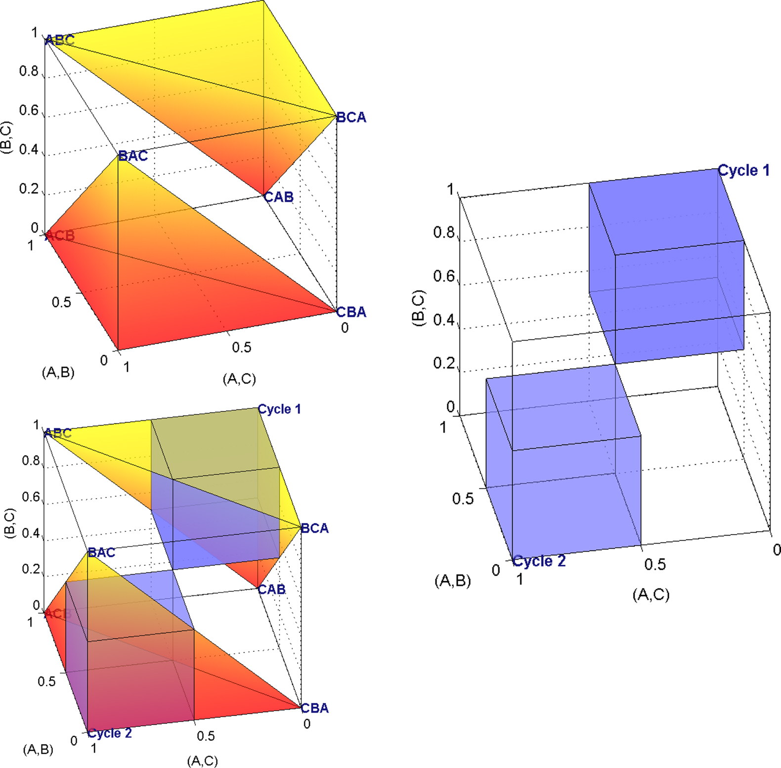
Figure 1. Upper left: The unshaded volume is the linear ordering polytope for m = 3. Upper right: The unshaded volume is weak stochastic transitivity for m = 3. Lower left: Both conditions shown together for comparison. Writing 𝒞 = {a,b,c}, the left hand side axis from front to back is P_ab, the vertical axis from bottom to top is P_bc, and the remaining axis, from right to left, is P_ac.

As we move to more than three choice alternatives, matters are complicated by the fact that the conditions in (12) are applicable to every possible triple of choice alternatives. Consider, for instance, m = 5, as in Tversky’s study. Taking all possible selections of x,y,z into account, (11) becomes a list of yes inequality triples, rather than the eight triples of inequalities of (12). Of these 80 triples of inequalities, 60 belong to H₀ (corresponding to the yes strict linear orders of three out of five objects) and 20 belong to H_A (corresponding to the yes cycles on three out of five objects). Now, we operate in a yes = 10-dimensional unit hypercube, and the two hypotheses partition that 10-dimensional unit hypercube into two nonconvex unions of half-unit hypercubes.

A major conceptual problem with violations of weak stochastic transitivity is the Condorcet paradox of social choice theory (Condorcet, 1785). Even though this crucial caveat has previously been brought up (Loomes and Sugden, 1995), it continues to be neglected by the literature. According to the Condorcet paradox, transitive individual preferences aggregated by majority rule can yield majority cycles. For example, consider a uniform distribution on the following three transitive strict linear orders B₁ ={(a,b),(b,c),(a,c)}, B₂ = {(b,c),(c,a),(b,a)}, and B₃ = {(c,a),(a,b),(c,b)}. This distribution has marginal probabilities

i.e. it violates weak stochastic transitivity.

Our discussion of weak stochastic transitivity so far shows that this approach confounds intransitivity with variability of preferences. Next, we note that weak stochastic transitivity also does not model transitivity in isolation from other axioms of preference.

First, it is well known that weak stochastic transitivity (11) is equivalent to the weak utility model (Block and Marschak, 1960; Luce and Suppes, 1965), according to which there exists a real-valued utility function u such that, ∀ (distinct) x,y ∈ 𝒞,

The first equivalence shows how weak stochastic transitivity establishes the existence of an aggregate ordinal utility function. Both, in turn, induce the aggregate preference relation ≿ (via Formula 10) that, in addition to being transitive, satisfies other axioms. Specifically, the aggregate preference relation ≿ is a weak order and the aggregate strict preference relation ≻ is a strict weak order on the set of choice alternatives.

Empirically and normatively, reflexivity may be more or less automatic, as it basically says that a decision maker is indifferent between any object x and the same object x (assuming that the decision maker recognizes it to be the same). However, Kramer and Budescu (2005) have provided evidence that preference in laboratory experiments is often not strongly complete. Likewise, we would argue that strong completeness is not a necessary property of rational preferences. For example, expected value maximizers are indifferent among lotteries with equal expected value. Negative transitivity implies transitivity in the presence of asymmetry, but it is stronger. As a consequence, a weak or strict weak order is violated as soon as any one of the axioms of weak and/or strict weak orders is violated, not necessarily transitivity.

The situation is even more grave. Recall that each vector of binomial probabilities translates into one single binary relation ≿ via (10). Figure 1 and Hypothesis Test (12) illustrate that, up to the knife-edge case where some probabilities P_xy, P_xz, or P_yz are equal to 1/2, weak stochastic transitivity only allows (10) to yield linear order preferences. Formally, in the parameter space for weak stochastic transitivity, the set of weak orders minus the set of linear orders is a set of measure zero. This means that in weak stochastic transitivity, up to a set of measure zero, we only consider (aggregate) linear order preferences [(via 10)]. These properties are substantially stronger than transitivity alone, especially for large m. For five objects, there are 120 possible linear orders, whereas there are 541 weak orders, 1012 partial orders, and altogether 154303 transitive relations (see, e.g. Klaška, 1997; Fiorini, 2001). From a geometric viewpoint and for five choice objects, weak stochastic transitivity, while technically permitting other transitive relations besides the 120 possible different linear orders, effectively gives measure zero (in the unit hypercube of binomial probabilities) to the remaining 421 weak orders, and completely neglects the enormous number of transitive relations that are not weak orders. Note that stronger versions of stochastic transitivity (Chen and Corter, 2006; Rieskamp et al., 2006), that use more information about the binary choice probabilities, imply models with even more structure.

Next, consider the disappointing feature that (10), and thus also weak stochastic transitivity, treats probability as a binary categorical scale rather than an absolute scale. Whether P_xy = 0.51 or 0.99, both cases are interpreted to mean that the participant prefers x to y. The mixture models we promote below use the binary choice probabilities on an absolute (probability) scale.

This concludes our multifaceted demonstration that violations of weak stochastic transitivity cannot legitimately be interpreted as demonstrations of intransitive individual preferences. Next, we discuss a more suitable modeling approach.

Mixture Models of Transitive Preference

We now consider a class of models that uses general tools for probabilistic generalizations of deterministic axioms or axiom systems (Heyer and Niederée, 1989, 1992; Regenwetter, 1996; Niederée and Heyer, 1997; Regenwetter and Marley, 2001) and that differs from the approaches we have seen so far. A mixture model of transitivity states that an “axiom-consistent” person’s response at any time point originates from a transitive preference state, but responses at different times need not be generated by the same transitive preference state. In the terminology of Loomes and Sugden (1995), this is a “random preference model” in that it takes a “core theory” (here, the axiom of transitivity) and considers all possible ways that the core theory can be satisfied. We use the term “mixture model” to avoid the misconception that “random preferences” would be uniformly distributed.

In the case of binary choices, again writing P_xy for the probability that a person chooses x over y, and writing 𝒯 for the collection of all transitive binary preference relations on 𝒞, the mixture model states that

where P_B is the probability that a person is in the transitive state of preference B∈𝒯. This does not assume 2AFC, i.e. P_xy + P_yx need not be 1. Equation (13) implies that intransitive relations have probability zero. This is the Null Hypothesis we considered in (7).

Even though the probability distribution over 𝒯 is not, in any way, constrained, neither this model nor weak stochastic transitivity of Formula (11) imply each other. This model implies other constraints on binary choice probabilities, such as, for instance, the triangle inequalities (Marschak, 1960; Morrison, 1963; Niederée and Heyer, 1997), i.e. for any distinct x,y,z∈𝒞:

The model stated in (13) is closely related to the more restrictive classical binary choice problem (e.g. Marschak, 1960; Niederée and Heyer, 1997). In that problem, each decision maker is required to have strict linear order preference states (not just transitive relations), and 𝒯 of (13) is replaced by the collection of linear orders over 𝒞, which we denote by Π:

This model requires P_xy + P_yx = 1. It implies a very restrictive special case of the Null Hypothesis in (7), namely a case where all binary relations, except the strict linear orders, have probability zero. We discussed (7) in the context of the multinomial sample space. When testing the restrictions on the marginal probabilities on the left side of (15) later, we will use a “products of binomials” sample space.

The model in (15) is equivalent to the (strict) linear ordering polytope (Grötschel et al., 1985; Fishburn and Falmagne, 1989; Cohen and Falmagne, 1990; Gilboa, 1990; Fishburn, 1992; Suck, 1992; Koppen, 1995; Bolotashvili et al., 1999; Fiorini, 2001). For each unordered pair {x,y} of distinct elements of 𝒞, arbitrarily fix one of the two possible ordered pairs associated with it, say (x,y). Now, for each (strict) linear order π∈Π, let π_xy = 1 if that ordered pair (x,y)∈π, and π_xy = 0, otherwise. Each strict linear order is thereby written as a 0/1 vector indexed by the previously fixed ordered pairs of elements in 𝒞, i.e. as a point in yes when |𝒞| = m. A probability distribution over strict linear orders can be mathematically represented as a convex combination of such 0/1 vectors, i.e. as a point in the convex hull of m! many points in yes . The linear ordering polytope is the resulting convex polytope whose vertices are the m! many 0/1 vectors associated with the strict linear orders.

Every convex polytope is an intersection of finitely many closed half spaces, each of which can be defined by an affine inequality. A minimal description of a convex polytope is a description by a shortest possible list of equations and inequalities. The inequalities in such a description are called facet-defining inequalities because they define the facets of the polytope, i.e. faces of maximal dimension.

The problem of characterizing binary choice probabilities induced by strict linear orders is still unsolved for large m. It is tantamount to determining all facet-defining inequalities of the linear ordering polytope for each m. Each triangle inequality (14) is facet-defining for the linear ordering polytope, for all m. For m ≤ 5, but not for m > 5, the triangle inequalities (14), together with the equations and canonical inequalities

P_xy + P_yx = 1 and 0 ≤ P_xy ≤ 1, ∀x,y ∈ 𝒞, x ≠ y,

provide a minimal description of the linear ordering polytope . In other words, they are necessary and sufficient for the binary choice probabilities to be consistent with a distribution over strict linear orders (Cohen and Falmagne, 1990; Fiorini, 2001).

Determining a minimal description of the linear ordering polytope is NP-complete. In other words, minimal descriptions can only be obtained in practice when the number of choice alternatives is fairly small. On the other hand, there exist some good algorithms to check whether or not a given point is inside the convex hull of a given finite set of points (e.g. Vapnik, 1995; Dulá and Helgason, 1996).

The 2AFC paradigm, where respondents must choose either of two offered choice alternatives, forces the data to artificially satisfy the strong completeness and asymmetry axioms in each observed paired comparison. In probability terms, the 2AFC paradigm forces the equations P_xy + P_yx = 1 to hold automatically. In other words, a canonical way to test whether binary forced-choice data satisfy a mixture over transitive relations is to test the stronger hypothesis that they lie in the (strict) linear ordering polytope, i.e. test whether (15) holds. Note, however, that violations of the linear ordering polytope, if found, cannot necessarily be attributed to violations of transitivity, because strict linear orders are much stronger than transitive relations.

For five gambles the triangle inequalities are necessary and sufficient for (15), and thus completely characterize the mixture over linear orders for such studies. For five objects, taking into account the quantifier, the triangle inequalities form a system of 20 different individual inequalities. For m > 5, the description of the linear ordering polytope becomes very complicated. According to Fiorini (2001), who provided a literature review of this and related polytopes, the case of m = 6 leads to two classes of facet-defining inequalities (including the triangle inequalities), that jointly form 910 inequality constraints, including the canonical inequalities. The case of m = 7 leads to six classes (including, again, the triangle inequalities) that jointly form 87,472 inequality constraints, whereas the case of m = 8 leads to over a thousand different inequality classes (including the triangle inequalities as just one such class) that jointly define at least 488 million inequalities slicing through the 28-dimensional unit hypercube.

An appealing feature of the linear order mixture model is that it can be equivalently cast in several alternative ways. We review this next.

Definition. Let 𝒞 be a finite collection of choice alternatives. A (distribution-free) random utility model for 𝒞 is a family of jointly distributed real random variables U = (U_c,i)_{c∈𝒞,i∈ℐ} with ℐ some finite index set.

The realization of a random utility model at some sample point ω, given by the real-valued vector (U_c,i(ω))_{c ∈𝒞,i ∈ℐ}, assigns to alternative c∈𝒞 the utility vector (U_c,i(ω))_{i ∈ℐ}. One possible interpretation of such a utility vector is that ℐ is a collection of attributes, and U_c,i(ω) is the utility of choice alternative c on attribute i at sample point ω.

Definition. Let 𝒞 be a finite collection of choice alternatives. A (distribution-free) unidimensional, noncoincident random utility model for 𝒞 is a family of jointly distributed real random variables U = (U_c)_c∈𝒞 with P(U_x = U_y) = 0, ∀x ≠ y ∈𝒞.

The most common use of the term “random utility model” in the Econometrics literature (e.g. Manski and McFadden, 1981; Ben-Akiva and Lerman, 1985; Train, 1986; McFadden, 2001) refers to parametric (unidimensional, noncoincident) models, where the random variables (U_c)_c∈𝒞 can be decomposed as follows:

and where U_c is the deterministic real-valued utility of option c and (E_c)_c∈𝒞 is multivariate normal or multivariate extreme value noise. One could argue that calling the representation (16) a “random utility model” is a bit odd, since it does not actually treat the utilities as random variables. However, modern extensions of (16) allow for latent classes or latent parameters to model variation in the utilities (see. e.g. Scott, 2006; Blavatskyy and Pogrebna, 2009). We do not investigate parametric models of the form (16) here. Rather, when we refer to random utility models in this paper, we have the general distribution-free model in mind, and we think of the utilities themselves as having some (unspecified, but fixed) joint distribution.

We now briefly explain the notion of “random function models” (Regenwetter and Marley, 2001). By a function on 𝒞, we mean a mapping from 𝒞 into the real numbers ℝ. The collection of all functions on 𝒞 is the space ℝ^𝒞. When 𝒞 contains n elements, this is ℝⁿ, the n-dimensional reals. Let ℬ(ℝ^𝒞) denote the sigma-algebra of Borel sets in ℝ^𝒞.

Definition. Let 𝒞 be a finite collection of choice alternatives. A random function model for 𝒞 is a probability space 〈ℝ^𝒞, ℬ(ℝ^𝒞), ℙ〉.

The idea behind a random function model is to define a (possibly unknown) probability measure ℙ on the space of (e.g. utility) functions on 𝒞. This space, of course, contains all conceivable unidimensional, real-valued, utility functions on 𝒞. We can now summarize key results about binary choice probabilities induced by linear orders, as given in (15).

Theorem. Consider a finite set 𝒞 of choice alternatives and a collection (P_xy)_{x,y∈𝒞,x ≠ y} of binary choice probabilities. The binary choice probabilities are induced by strict linear orders if and only if they are induced by a (distribution-free) unidimensional, noncoincident random utility model (Block and Marschak, 1960). Furthermore, this holds if and only if they are induced by a (distribution-free) random function model in the space of one-to-one functions (Regenwetter and Marley, 2001). Mathematically,

with suitable choices of probabilities and random variables on the right hand side.

The results above show that, for 2AFC, the following are equivalent: The binary choice probabilities are

• induced by a mixture model over linear orders, i.e. by a probability distribution over linear orders,

• consistent with a random preference model whose core theory states that preference is a linear order of the alternatives,

• a point in the linear ordering polytope,

• induced by a unidimensional, noncoincident random utility model,

• induced by a random function model with exclusively one-to-one (utility) functions.

Thurstonian models (with independent or dependent multivariate normal distributions) are parametric special cases of noncoincident random utility models, and, hence, as nested submodels of the linear ordering polytope, imply that the triangle inequalities (14) must hold. Some extensions, such as those of Takane (1987) and Tsai and Böckenholt (2006), allow nonzero probability mass on nontransitive binary relations, – see also Maydeu-Olivares and Hernández (2007) for further discussion on this point. These are not nested in the linear ordering polytope and, hence, do not imply the triangle inequalities.

Informally, the mixture, random utility and random function models for 2AFC state that decision makers may be in different mental states at different time points. Each mental state has three different but equivalent interpretations (with the third forming the link between the first two): (1) In any given permissible mental state, the decision maker’s preferences form a strict linear order over the alternatives. (2) In each mental state, the decision maker’s utility of a strictly preferred option strictly exceeds the utility of the less preferred option. (3) In each mental state the decision maker has a one-to-one real-valued utility function over the set of alternatives that assigns strictly higher utilities to strictly preferred alternatives.

To summarize, we can model variability of preferences and choice (or uncertainty of preferences und choice) by placing a probability measure on the collection of mental states and by assuming that individual observations are randomly sampled from the space of mental states. Noncoincidence of the random utilities and “one-to-one”-ness of the utility functions means that two distinct choice alternatives have equal utility with probability zero, i.e. indifference occurs with probability zero. This feature of the model accommodates the 2AFC paradigm, in which expressing indifference is not permitted.

Weak Stochastic Transitivity Versus the Linear Ordering Polytope

Some researchers (e.g. Loomes and Sugden, 1995, p. 646) have suggested that the triangle inequalities are less restrictive than weak stochastic transitivity. To differentiate mathematically and conceptually between weak stochastic transitivity as an aggregate operationalization of transitive preference and the linear ordering polytope as a disaggregate operationalization, it is useful to compare the parameter spaces of the two models geometrically, by considering how they are embedded in the 2AFC sample space. Recall that, for m many alternatives, the sample space that uses yes many binomial probabilities can be identified by the yes dimensional unit hypercube.

For instance, for 2AFC among three alternatives, viewed in three-space, the sample space forms a three-dimensional unit cube. The sample space and the two parameter spaces for the three-alternative case are displayed in Figure 1. Weak stochastic transitivity (11) rules out two half-unit cubes of the three-dimensional unit cube (upper right quadrant). The triangle inequalities (14), which characterize the linear ordering polytope, rule out two pyramids, as shown in the upper left quadrant of Figure 1. Here, and in general, the linear ordering polytope is a convex set, whereas weak stochastic transitivity is a nonconvex union of convex sets.

The inadmissible regions of the two models overlap, as shown in the lower left quadrant in Figure 1 for the three-dimensional case. They include the same two vertices of the unit cube, namely the vertices whose coordinates correspond to the two perfect cycles on three objects. Thus, Tversky (1969) and others’ operationalization of transitive preference via weak stochastic transitivity and the operationalization via mixture models, overlap to some degree. However, for three alternatives, weak stochastic transitivity constrains the parameter space to 3/4 of the volume of the unit cube, whereas the triangle inequalities constrain the parameter space to only 2/3 of the volume of the unit cube. The corresponding volumes for three, four, or five alternatives, as well as the volume of the overlap, are shown in Table 1. The triangle inequalities characterizing the linear ordering polytope when m ≤ 5 are more restrictive than weak stochastic transitivity. For five choice alternatives (as is the case, for instance, in Tversky’s study) the binary choice polytope defines a parameter space that only occupies 5% of the sample space, in contrast to Loomes and Sugden (1995) remark (p. 646) that the random preference model is “difficult to reject.” We conjecture that, for m > 5, the mixture model’s volume will shrink much faster than that of weak stochastic transitivity. We later provide an illustrative example, in which we test both models against empirical choice data.

TABLE 1

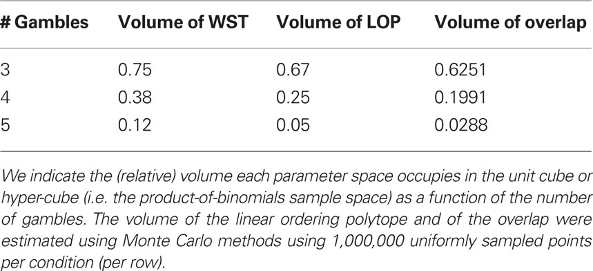
Table1. A comparison of the parsimony of weak stochastic transitivity (WST) and the linear ordering polytope (LOP), as well as their overlap (i.e. the volume of their intersection).

Statistical Methods for Testing Models of the Axiom of (Preference) Transitivity

In this section, we discuss how the literature tackles Luce’s second challenge, namely that of using adequate statistical methods. Here, much of the transitivity literature has been tripped by critical hurdles, but very substantial progress has also been made recently in the model testing literature.

Some papers on intransitive preferences used no statistical test at all (e.g. Brandstätter et al., 2006). The following sections highlight five major, and somewhat interconnected, problems with the statistical tests employed in the literature.

The Problem of Ignoring the Quantifier

A common approach concentrated on only one cycle, and attempted to show that the data satisfied that cycle (e.g. Shafir, 1994; McNamara and Diwadkar, 1997; Waite, 2001; Bateson, 2002; Schuck-Paim and Kacelnik, 2002). For example, the statement

is not a precise statement for the axiom of transitivity, because it omits the quantifier (∀x,y,z∈𝒞) that would be required for (20) to match (1). This imprecise statement led some researchers to incorrectly formulate weak stochastic transitivity as

In the case where m = 5, (21) shrinks the Null Hypothesis in (11) from 60 triples of inequalities to one, and the Alternative Hypothesis from 20 such triples down to one. Thus, calling (21) a “test of weak stochastic transitivity” is incorrect.

Moving beyond triples, some authors specified one particular intransitive relation (e.g. one particular “lexicographic semiorder”) and, within the binomial sample space framework, tried to show that the majority choices were consistent with that intransitive relation. In other words, they attempted to provide evidence that the binomial choice probabilities generating the data belonged to a particular one of the various half-unit hypercubes whose union makes up the Alternative Hypothesis in (11). If m = 5, for instance, this means that, instead of considering a union of 904 half-unit hypercubes, they concentrated on only one half-unit hypercube. Sometimes, the intransitive relation in question, say, a lexicographic semiorder, naturally reflected certain features in the design of the experiment. In that case, the hypothesis test was really a test of a parsimonious model of a particular type of intransitivity, and served as a test of transitivity only indirectly.

It is important to acknowledge that some papers in this area were not primarily aimed at testing transitivity. Calling such a test a “test of weak stochastic transitivity” would, indeed, be a misnomer: (1) Failing to fit that intransitive relation (say, a lexicographic semiorder) has no bearing on whether weak stochastic transitivity is satisfied or violated. (2) Likewise, if the half-unit hypercube attached to the intransitive relation can account for the data, then its goodness-of-fit is not a significance level for violations of weak stochastic transitivity. Both of these insights follow from the fact that a single half-unit hypercube in the Alternative Hypothesis in (11) and weak stochastic transitivity, the Null in (11), do not form two collectively exhaustive events.

The Problem of Multiple Binomial Tests

Within the framework of the binomial sample space approach it is common to carry out multiple binomial tests (e.g. Shafir, 1994; McNamara and Diwadkar, 1997; Waite, 2001; Schuck-Paim and Kacelnik, 2002). This corresponds geometrically to checking separately whether each individual binomial probability lies on one side or the other of a separating hyperplane that cuts the unit hypercube in half. Whether one wants to compute the goodness-of-fit for a single, theoretically motivated half-unit hypercube (say, associated with a particular lexicographic semiorder) or try to establish which of the possible half-unit hypercubes best accounts for the data, that test should not be carried out with a series of separate binomial tests, because this leads to a proliferation of Type-I error.

In the case of a prespecified half-unit hypercube, all binomial probabilities associated with the half-unit hypercube should be tested jointly. Similarly, testing weak stochastic transitivity requires testing a nonconvex union of hypercubes, all at once. In general, all binomial restrictions can and should be tested jointly, as discussed in the next section.

The Boundary Problem in Constrained Inference

Iverson and Falmagne (1985) showed the fact we reviewed above: weak stochastic transitivity characterizes a nonconvex parameter space. The fact that it is a nonconvex union of half-unit hypercubes embedded in the unit hypercube makes parameter estimation tricky. Furthermore, the log-likelihood ratio test statistic in maximum likelihood estimation does not have an asymptotic χ² distribution. Tversky (1969) tried to accommodate the latter fact, but did not succeed: As Iverson and Falmagne (1985) showed, all but one of Tversky’s violations of weak stochastic transitivity turned out to be statistically nonsignificant when analyzed with an appropriate asymptotic sampling distribution. Boundary problems, similar to those for stochastic transitivity, have recently been tackled in very general ways (see the new developments in order constrained inference of Myung et al., 2005; Davis-Stober, 2009).

The Problem of Statistical Significance with Pre-Screened Participants

One more complicating feature of Tversky (1969) study (as well as of, e.g. Montgomery, 1977; Ranyard, 1977) is the fact that Tversky pre-screened the respondents before the study. For instance, out of 18 volunteers, eight persons participated in Experiment 1 after having been evaluated as particularly prone to “intransitive” (or inconsistent) behavior in a pilot study. If any violations of weak stochastic transitivity (or some other probabilistic model) were to be found, this feature would raise the philosophical question of what population these participants were randomly sampled from. Similar questions arise in the context of cherry-picked stimuli.

Maximum Likelihood Estimation Subject to the Linear Ordering Polytope

Maximum likelihood estimation consists of searching for model parameter values so as to maximize the likelihood function (in our case, Formula 4). To evaluate the goodness-of-fit, we need to obtain the maximum likelihood estimators for the unconstrained model (the unit cube in yes dimensions) and for the constrained model (the linear ordering polytope). In the unconstrained model, the maximum likelihood estimator of this model is the vector of observed choice proportions Q = (Q_xy)_{x,y∈𝒞,x ≠ y}. This elementary result from mathematical statistics follows readily by setting the necessary partial derivatives of the log-likelihood with respect to P_xy equal to zero and solving the resulting system of equations. Under the linear ordering polytope for binary choices we have a fully parameterized space that is completely described by the polytope’s facet-defining inequalities.

As the mixture model is constrained by the linear ordering polytope, if an observed vector of choice proportions (mapped into the unconstrained space) falls outside of the polytope, the maximum likelihood estimator is no longer the vector of observed choice proportions. Hence, we must compute the maximum likelihood estimator in a different fashion.

The linear ordering polytope is a closed and convex set, hence the maximum likelihood estimator for these data is guaranteed to exist and to be unique (since the log-likelihood function is concave over the linear ordering polytope, which is itself a convex set). The problem of maximizing the log-likelihood function subject to the triangle inequalities can now be reformulated in terms of nonlinear optimization. Specifically, given an observed vector of choice proportions Q, the task is to maximize the log-likelihood function such that the choice parameters lie within the linear ordering polytope. In other words, we need to find yes that maximizes the likelihood function yes in (4), subject to the constraint that yes must lie in the linear ordering polytope. This maximization can be carried out using a standard nonlinear optimization routine. For our analysis we used the optimization toolkit of the MATLAB^© computer software package.

We face a constrained inference problem, where the log-likelihood ratio test statistic fails to have an asymptotic χ² distribution when the observed choice proportions lie outside the polytope, because the point estimate will lie on a face of the polytope – thus violating a critical assumption for asymptotic convergence of the likelihood ratio test. Instead, we need to use a yes distribution whose weights depend on the local geometric structure of the polytope around the point estimate. Davis-Stober (2009) provides a methodology to carry out this test within the context of the linear ordering polytope. We used his method and refer the reader to that paper for the technical details.

Illustrative Examples

Regenwetter et al. (2011) showed that 18 participants, across three different five-gamble stimulus sets, were consistent with the linear ordering polytope up to sampling variability and Type-I error. Their stimulus sets were labeled “Cash I,” “Cash II,” and “Noncash” conditions, reflecting that the first two featured cash gambles, whereas the third featured gambles with noncash prizes as outcomes. In Table 2, we abbreviate these with e.g. “1/CII” referring to “Respondent 1” in the “Cash II” condition, and “2/NC” referring to “Respondent 2” in the “Noncash” condition.

TABLE 2

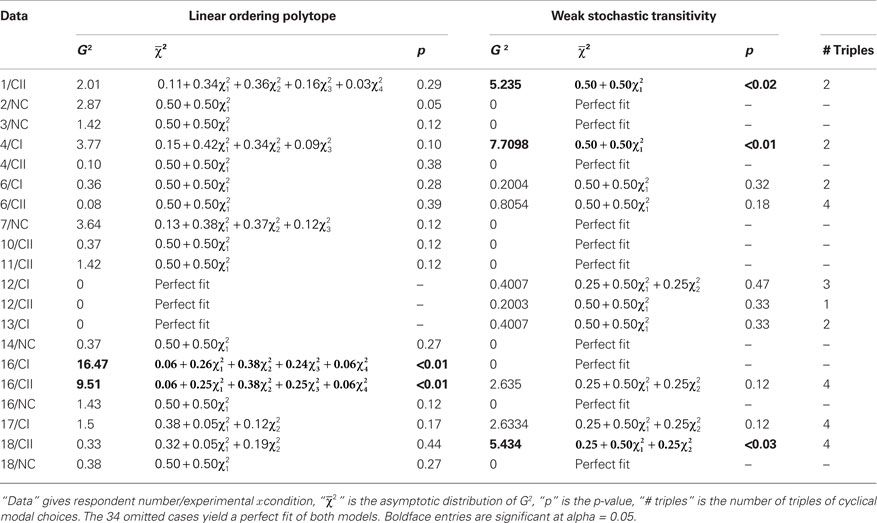
Table 2. Goodness-of-fit of the linear ordering polytope and weak stochastic transitivity.

We complement the linear ordering polytope analysis of Regenwetter et al. (2011) with a more fine-tuned analysis using an updated algorithm to compute the goodness-of-fit along the lines of Davis-Stober (2009). We also use the same method to test weak stochastic transitivity. This test has its roots in earlier work by Iverson and Falmagne (1985), who derived the most conservative yes distribution for weak stochastic transitivity with respect to a likelihood ratio test.

Strikingly, out of 54 respondent-stimulus set combinations, 34 lead to a perfect fit of both models. In other words, 34 of 54 data sets are consistent with the idea that both instantaneous and aggregated preferences are transitive linear orders! All those 34 data sets fit so well that a statistical test is superfluous.

Table 2 shows a summary of the goodness-of-fit for both the LOP and WST for the remaining 20 cases, where at least one model does not have a perfect fit. When evaluated with the asymptotic yes distribution of Davis-Stober (2009), weak stochastic transitivity turns out to be significantly violated (as indicated in Table 2) in only three cases at α = 0.05. Like the two significant violations of the linear ordering polytope, this is roughly the rate of violations one would expect by Type-I error alone. Hence, it appears that our respondents’ preferences are consistent with linear order preferences at the disaggregate level (linear order preferences), as well as with weak order preferences at the majority rule aggregate level (weak stochastic transitivity).

Altogether 44 out of 54 data sets give point estimates in the interior of weak stochastic transitivity, where the majority aggregated preferences are even linear orders. The ten nonsignificant violations yield knife-edge distributions, with one or more majority ties, as point estimates. These point estimates lie on faces (of half-unit hypercubes) forming the boundary between the Null and the Alternative Hypothesis in (11). Even if these choice proportions are generated from a point in the interior of a half-unit cube (i.e. from a linear order), the geometry of weak stochastic transitivity automatically forces the point estimate to lie on the parameter space boundary (i.e. yield a weak order that is not a linear order).

Table 2 also documents an important pattern counting problem for weak stochastic transitivity: The number of cyclical modal choice triples (x,y,z) where x was chosen over y most of the time, y was chosen over z most of the time, z was chosen over x most of the time, is not monotonically related to the goodness-of-fit (or the p-value) of weak stochastic transitivity. For example, sets 1/CII and 4/CI violate WST significantly, each with two cyclical modal choice triples, whereas 6/CII, 16/CII, and 17/CII yield a good quantitative fit despite four cyclical modal choice triples. This is another reminder that pattern counting is diagnostic of neither goodness-of-fit nor of significance of violation.

Last, but not least, recall from Table 1 that the intersection of LOP and WST occupies 2.88% of the space of binomial probabilities (for five choice alternatives). Empirically, we find 49 out of 54 data sets fit by both models (in separate tests), including 34 that fit perfectly. It is interesting to notice that the three significant violations of WST are for data where LOP is not significantly violated, hence these three out of 54 data sets yield evidence of Condorcet paradoxes (but only at a rate consistent with Type-I error). Note that Regenwetter et al. (2011) carried a power study that suggests that we have sufficient power to reject the LOP when it is violated.

Discussion

Several researchers have highlighted the conceptual, mathematical, and statistical gap between algebraic axioms underlying scientific theory on the one hand, and variable empirical data on the other hand. We have labeled this problem “Luce’s challenge” to pay tribute to mathematical psychologist R. Duncan Luce, who pioneered potential solutions to this problem with his famous choice axiom (Luce, 1959) and who continued to highlight the importance of probabilistic specification throughout his illustrious career.

To summarize our conclusions, here are the major steps that one must take to empirically test the axiom of transitivity:

1. Understand the empirical sample space of possible observations.

We work within a binomial sample space that assumes the number of times x is chosen over y is a binomial random variable with N repetitions and probability of success P_xy. Thus, the sample space is a unit hypercube of dimension yes , representing the binomial probabilities for all unique pairs of choice alternatives. Working at the level of the binomial sample space allows the researcher to use, e.g. 5 choice alternatives, making transitivity a rather parsimonious hypothesis, while maintaining a manageable number of parameters to estimate. We are thus relying on the assumption of iid sampling. Because we do not recommend pooling data across individuals, the data are repeated binary choices by the same respondent. Here, it is important to take measures that make the iid sampling assumption more realistic, such as using decoys and forcing respondents to make pairwise choices one at a time without going back to previous choices.

2. Formulate a probabilistic statement of transitivity. We endorse the mixture model as a conception of variability in choice behavior. In the 2AFC paradigm, the mixture model implies the triangle inequalities in (14). We endorse this formulation over the more commonly used weak stochastic transitivity because it is free of aggregation paradoxes, treats probabilities as continuous, and is more restrictive. The allowable parameter space for transitivity is thus the linear ordering polytope within the unit hypercube.

3. Properly test the probabilistic formulation of transitivity on data.

• If the choice proportions in a 2AFC experiment fall within the linear ordering polytope, i.e. do not violate the triangle inequalities, then transitivity is a perfect fit and no further testing is required.

• If the choice proportions violate the triangle inequalities, the maximum likelihood estimate of the binomial choice probabilities is not simply the observed choice proportions. The researcher must then obtain the MLE and conduct a constrained inference test with the appropriate yes distribution to determine if the choice vector significantly violates the linear ordering polytope. The testing procedure for the linear ordering polytope within the unit hypercube is described in Davis-Stober (2009).

Finally, as we have seen and as we also explain in Regenwetter et al. (2011), the 2AFC paradigm does not test transitivity in isolation. If a set of data were to reject the linear ordering polytope, this would mean that the combination of strong completeness, asymmetry and transitivity is violated. A more direct test of transitivity requires a different empirical paradigm.

The mixture model approach can be extended to other algebraic axioms and/or to other empirical paradigms. In each case, there are several steps towards a successful solution of Luce’s challenge: First, one needs to fully characterize the sample space under consideration. Second, we anticipate that probabilistic specification of other axioms through mixture (random preference) models will typically lead to convex polytopes again. These, in turn, can sometimes be prohibitively hard to characterize, but sometimes complete minimal descriptions can be obtained analytically or via public domain software. Third, to the extent that future probabilistic specifications of algebraic axioms take the form of convex polytopes or unions of convex polytopes, researchers will have to tackle the problem of order constrained inference that is intimately attached to such endeavors when analyzing empirical data. Fortunately, this is a domain where much progress has been made in recent years, with the provision of both frequentist and Bayesian solutions that are applicable to a broad array of problems, as long as the inequality constraints are completely and explicitly known.

There are also a variety of interesting open problems in this domain. What are suitable empirical paradigms that go more directly after transitivity, without the burden of auxiliary modeling or statistical assumptions? One open question concerns the assumption of iid sampling. Are there relaxations of this assumption that will not force the researcher to revert to the multinomial sample space, or even the universal sample space? Recall that both of these entail combinatoric explosions in the empirical degrees of freedom. Likewise, how robust is the analysis against violations of the underlying assumptions? Do any conclusions change in a Bayesian analysis, and does such an analysis perform well with small sample size? These are but a few of the interesting methodological research questions that arise for follow-up work.

Looking beyond individual axioms, many theories in psychology have been axiomatized by mathematical psychologists. When testing such theories, we are usually dealing with conjunctions of axioms, and hence with a variety of Luce’s challenge. Elsewhere we develop a general framework and public domain software package to handle several types of probabilistic specifications for such situations.

Conflict of Interest Statement

The authors declare that the research was conducted in the absence of any commercial or financial relationships that could be construed as a potential conflict of interest.

Acknowledgments

Special thanks to William Batchelder, Michael Birnbaum, Ulf Böckenholt, David Budescu, Jerome Busemeyer, Jean-Paul Doignon, Jean-Claude Falmagne, Klaus Fiedler, Samuel Fiorini, Jürgen Heller, Geoffrey Iverson, David Krantz, Graham Loomes, Duncan Luce, Tony Marley, John Miyamoto, Reinhard Suck, and Peter Wakker (as well as thanks to many others) for helpful comments, pointers and/or data.

This material is based upon work supported by the Air Force Office of Scientific Research, Cognition and Decision Program, under Award No. FA9550-05-1-0356 entitled “Testing Transitivity and Related Axioms of Preference for Individuals and Small Groups” (to M. Regenwetter, PI), by the National Institutes of Mental Health under Training Grant Award Nr. PHS 2 T32 MH014257 entitled “Quantitative Methods for Behavioral Research” (to M. Regenwetter, PI), and by the Decision, Risk and Management Science Program of the National Science Foundation under Award No. SES #08-20009 (to M. Regenwetter, PI) entitled “A Quantitative Behavioral Framework for Individual and Social Choice.” Much of this paper was written while the first author was a Fellow of the Max Planck Institute for Human Development (ABC group), and while the third author was the recipient of a Dissertation Completion Fellowship of the University of Illinois. Any opinions, findings, and conclusions or recommendations expressed in this publication are those of the authors and do not necessarily reflect the views of universities, funding agencies or individuals who have provided comments.

References

Bateson, M. (2002). Context-dependent foraging choices in risk-sensitive starlings. Anim. Behav. 64, 251–260.