Perceptions as Hypotheses: Saccades as Experiments

If perception corresponds to hypothesis testing (Gregory, 1980); then visual searches might be construed as experiments that generate sensory data. In this work, we explore the idea that saccadic eye movements are optimal experiments, in which data are gathered to test hypotheses or beliefs about how those data are caused. This provides a plausible model of visual search that can be motivated from the basic principles of self-organized behavior: namely, the imperative to minimize the entropy of hidden states of the world and their sensory consequences. This imperative is met if agents sample hidden states of the world efficiently. This efficient sampling of salient information can be derived in a fairly straightforward way, using approximate Bayesian inference and variational free-energy minimization. Simulations of the resulting active inference scheme reproduce sequential eye movements that are reminiscent of empirically observed saccades and provide some counterintuitive insights into the way that sensory evidence is accumulated or assimilated into beliefs about the world.

Introduction

This paper continues our effort to understand action and perception in terms of variational free-energy minimization (Friston et al., 2006). The minimization of free energy is based on the assumption that biological systems or agents maximize the Bayesian evidence for their model of the world through an active sampling of sensory information. In this context, negative free energy provides a proxy for model evidence that is much easier to evaluate than evidence per se. Under some simplifying assumptions, free-energy reduces to the amount of prediction error. This means that minimizing free-energy corresponds to minimizing prediction errors and can be formulated as predictive coding (Rao and Ballard, 1999; Friston, 2005). Expressed like this, minimizing free-energy sounds perfectly plausible and fits comfortably with Bayesian treatments of perception (Knill and Pouget, 2004; Yuille and Kersten, 2006). However, log model evidence is the complement of self information or surprise in information theory. This means that maximizing evidence corresponds to minimizing surprise; in other words, agents should sample their world to preclude surprises. Despite the explanatory power of predictive coding as a metaphor for perceptual inference in the brain, it leads to a rather paradoxical conclusion: if we are trying to minimize surprise, we should avoid sensory stimulation and retire to a dark and quiet room.

This is the dark room problem and is often raised as a natural objection to the principle of free-energy minimization. In Friston et al. (2012), we rehearse the problem and its implications in the form of a three-way conversation between a physicist, a philosopher, and an information theorist. The resolution of the dark room problem is fairly simple: prior beliefs render dark rooms surprising. The existence of these beliefs is assured by natural selection, in the sense that agents that did not find dark rooms surprising would stay there indefinitely, until they die of dehydration or loneliness. However, this answer to the darkroom paradox does not tell us very much about the nature or principles that determine the prior beliefs that are essential for survival. In this paper, we consider prior beliefs more formally using information theory and the free-energy formulation and specify exactly what these prior beliefs are optimizing. In brief, we will see that agents engage actively with their sensorium and must be equipped with prior beliefs that salient features of the world will disclose themselves, or be discovered by active sampling. This leads to a natural explanation for exploratory behavior and visual search strategies, of the sort studied in psychology and psychophysics (Gibson, 1979; Itti and Koch, 2001; Humphreys et al., 2009; Itti and Baldi, 2009; Shires et al., 2010; Shen et al., 2011; Wurtz et al., 2011). Crucially, this behavior is an emergent property of minimizing surprise about sensations and their causes. In brief, this requires an agent to select or sample sensations that are predicted and believe that this sampling will minimize uncertainty about those predictions.

The prior beliefs that emerge from this formulation are sensible from a number of perspectives. We will see that they can be regarded as beliefs that sensory information is acquired to minimize uncertainty about its causes. These sorts of beliefs are commonplace in everyday life and scientific investigation. Perhaps the simplest example is a scientific experiment designed to minimize the uncertainty about some hypothetical mechanism or treatment effect (Daunizeau et al., 2011). In other words, we acquire data we believe will provide evidence for (or against) a hypothesis. In a psychological setting, if we regard perception as hypothesis testing (Gregory, 1980), this translates naturally into an active sampling of sensory data to disclose the hidden objects or causes we believe are generating those data. Neurobiologically, this translates to optimal visual search strategies that optimize the salience of sampling; where salience can be defined operationally in terms of minimizing conditional uncertainty about perceptual representations. We will see that prior beliefs about the active sampling of salient features are exactly consistent with the maximization of Bayesian surprise (Itti and Baldi, 2009), optimizing signal detection (Morgan, 2011), the principle of minimum redundancy (Barlow, 1961), and the principle of maximum information transfer (Linsker, 1990; Bialek et al., 2001).

From the point of view of the free-energy principle, a more detailed examination of prior beliefs forces us to consider some important distinctions about hidden states of the world and the controlled nature of perceptual inference. In short, free-energy minimization is applied to both action and perception (Friston, 2010) such that behavior, or more simply movement, tries to minimize prediction errors, and thereby fulfill predictions based upon conditional beliefs about the state of the world. However, the uncertainty associated with those conditional beliefs depends upon the way data are sampled; for example, where we direct our gaze or how we palpate a surface. The physical deployment of sensory epithelia is itself a hidden state of the world that has to be inferred. However, these hidden states can be changed by action, which means there is a subset of hidden states over which we have control. These will be referred to as hidden controls states or more simply hidden controls. The prior beliefs considered below pertain to these hidden controls and dictate how we engage actively with the environment to minimize the uncertainty of our perceptual inferences. Crucially, this means that prior beliefs have to be encoded physically (neuronally) leading to the notion of fictive or counterfactual representations; in other words, what we would infer about the world, if we sample it in a particularly way. This leads naturally to the internal representation of prior beliefs about fictive sampling and the emergence of things like intention and salience. Furthermore, counterfactual representations take us beyond predictive coding of current sensations and into prospective coding about our sensory behavior in the future. This prospective coding rests on an internal model of control (control states) that may be an important element of generative models that endow agents with a sense of agency. This is because, unlike action, hidden controls are inferred, which requires a probabilistic representation of control. We will try to illustrate these points using visual search and the optimal control of saccadic eye movements (Grossberg et al., 1997; Itti and Baldi, 2009; Srihasam et al., 2009); noting that similar principles should apply to active sampling of any sensory inputs. For example, they should apply to motor control when making inferences about objects causing somatosensory sensations (Gibson, 1979).

This paper comprises four sections. In the first, we focus on theoretical aspects and describe how prior beliefs about hidden control states follow from the basic imperatives of self organization (Ashby, 1947). This section uses a general but rather abstract formulation of agents, in terms of the states they can occupy, that enables us to explain action, perception, and control as corollaries of a single principle. The particular focus here will be on prior beliefs about control and how they can be understood in terms of more familiar constructs such as signal detection theory, the principle of maximum mutual information and specific treatments of visual attention such as Bayesian surprise (Itti and Baldi, 2009). Having established the underlying theory, the second section considers neurobiological implementation in terms of predictive coding and recurrent message passing in the brain. This brief section reprises the implicit neural architecture we have described in many previous publications and extends it to include the encoding of prior beliefs in terms of (place coded) saliency maps. The third and fourth sections provide an illustration of the basic ideas using neuronally plausible simulations of visual search and the control of saccadic eye movements. This illustration allows us to understand Bayes-optimal searches in terms of saliency maps and the saltatory accumulation of evidence during perceptual categorization. We conclude with a brief discussion of the theoretical implications of these ideas and how they could be tested empirically.

Action, Perception, and Control

This section establishes the nature of Bayes-optimal inference in the context of controlled sensory searches. It starts with the basic premise that underlies free-energy minimization; namely, the imperative to minimize the dispersion of sensory states and their hidden causes to ensure a homeostasis of the external and internal milieu (Ashby, 1947). It shows briefly how action and perception follow from this imperative and highlights the important role of prior beliefs about the sampling of sensory states.

This section develops the ideas in a rather compact and formal way. Readers who prefer a non-mathematical description could skip to the summary and discussion of the main results at the end of this section. For people familiar with the free-energy formulation, this paper contains an important extension or generalization of the basic account of action and perception: here, we consider not just the minimization of sensory surprise or entropy but the entropy or dispersion of both sensory states and the hidden states that cause them. In brief, this leads to particular prior beliefs about the active sampling of sensory states, which may offer an explanation for the nature of sensory searches.

Notation and Set up

We will use X: $\Omega \times \dots$ → ℝ for real valued random variables and x ∈ X for particular values. A probability density will be denoted by p(x) = Pr{X = x} using the usual conventions and its entropy H[p(x)] by H(X). The tilde notation $\tilde{x}=\left(x,x^{\prime },x^{″},\dots \right)$ denotes variables in generalized coordinates of motion (Friston, 2008), where each prime denotes a temporal derivative (using Lagrange’s notation). For simplicity, constant terms will be omitted from equalities.

In what follows, we would consider free-energy minimization in terms of active inference: Active inference rests on the tuple (Ω, ψ, S, A, R, q, p) that comprises the following:

• A sample space Ω or non-empty set from which random fluctuations or outcomes ω ∈ Ω are drawn.

• Hidden states Ψ:Ψ × A × Ω → ℝ that constitute the dynamics of states of the world that cause sensory states and depend on action.

• Sensory states S:Ψ × A × Ω → ℝ that correspond to the agent’s sensations and constitute a probabilistic mapping from action and hidden states.

• Action A:S ×R → ℝ corresponding to an agent’s action that depends on its sensory and internal states.

• Internal states R:R × S × Ω → ℝ that constitute the dynamics of states of the agent that cause action and depend on sensory states.

• Conditional density $q\left(\tilde{\psi }\right):=q\left(\tilde{\psi }|\tilde{\mu }\right)$ – an arbitrary probability density function over hidden states $\tilde{\psi }\in \psi$ that is parameterized by internal states $\tilde{\mu }\in R.$

• Generative density $p\left(\tilde{s},\tilde{\psi }|m\right)$ – a probability density function over sensory and hidden states under a generative model denoted by m.

We assume that the imperative for any biological system is to minimize the dispersion of its sensory and hidden states, with respect to action (Ashby, 1947). We will refer to the sensory and hidden states collectively as external states S × Ψ. Mathematically, the dispersion of external states corresponds to the (Shannon) entropy of their probability density that, under ergodic assumptions, equals (almost surely) the long-term time average of Gibbs energy:

$\begin{array}{c}H\left(S,\Psi \right)=E_t\left[G\left(\tilde{s}\left(t\right),\tilde{\psi }\left(t\right)\right)\right]\\ G=-lnp\left(\tilde{s}\left(t\right),\tilde{\psi }\left(t\right)|m\right)\end{array}$(1)

Gibbs energy $G\left(\tilde{s},\tilde{\psi }\right)$ is defined in terms of the generative density or model. Clearly, agents cannot minimize this energy directly because the hidden states are unknown. However, we can decompose the entropy into the entropy of the sensory states (to which the system has access) and the conditional entropy of hidden states (to which the system does not have access)

$\begin{array}{l}H\left(S,\Psi \right)=H\left(S\right)+H\left(\Psi |S\right)\\ =E_t\left[-lnp\left(\tilde{s}\left(t\right)|m\right)+H\left(\Psi |S=\tilde{s}\left(t\right)\right)\right]\end{array}$(2)

This means that the entropy of the external states can be minimized through action to minimize sensory surprise $-lnp\left(\tilde{s}\left(t\right)|m\right),$ under the assumption that the consequences of action minimize conditional entropy:

$\begin{array}{c}a\left(t\right)=\underset{a\in A}{argmin}\left\{-lnp\left(\tilde{s}\left(t\right)|m\right)\right\}ũ\left(t\right)=\underset{ũ\in U}{argmin}\left\{H\left(\Psi |S=\tilde{s}\left(t\right)\right)\right\}\end{array}$(3)

The consequences of action are expressed by changes in a subset of external states U ⊂ Ψ, that we will call hidden control states or hidden controls. When Eq. 3 is satisfied, the variation of entropy in Eq. 1 with respect to action and its consequences are zero, which means the entropy has been minimized (at least locally). However, the hidden controls cannot be optimized explicitly because they are hidden from the agent. To resolve this problem, we first consider action and then return to optimizing hidden controls post hoc.

Action and Perception

Action cannot minimize sensory surprise directly (Eq. 3) because this would involve an intractable marginalization over hidden states, so surprise is replaced with an upper bound called variational free energy (Feynman, 1972). This free energy is a functional of the conditional density or a function of its parameters and is relatively easy to evaluate. However, replacing surprise with free energy means that internal states also have to minimize free energy, to ensure it is a tight bound on surprise:

$\begin{array}{l}\begin{array}{c}a(t)=\arg \min \{F(\tilde{s}(t),\tilde{\mu }(t))\}\\ a\in A\end{array}\\ \begin{array}{c}\tilde{\mu }(t)=\arg \min \{F(\tilde{s}(t),\tilde{\mu })\}\\ \tilde{\mu }\in R\end{array}\\ F=E_q\left[G(\tilde{s},\tilde{\psi })\right]-H\left[q(\tilde{\psi }|\tilde{\mu })\right]\\ =-\ln p(\tilde{s}|m)+D\left[q(\tilde{\psi })\left|\right|p\left(\tilde{\psi }|\tilde{s},m\right)\right]\\ \ge -\ln p(\tilde{s}|m)\end{array}$(4)

This induces a dual minimization with respect to action and the internal states that parameterize the conditional density. These minimizations correspond to action and perception respectively. In brief, the need for perception is induced by introducing free energy to finesse the evaluation of surprise; where free energy can be evaluated by an agent fairly easily, given a Gibbs energy or a generative model. The last equality says that free energy is always greater than surprise because the second (Kullback–Leibler divergence) term is non-negative. This means that when free energy is minimized with respect to the internal states, free-energy approximates surprise and the conditional density approximates the posterior density over external states:

$D\left[q\left(\tilde{\psi }\right)\left|\right|p\left(\tilde{\psi }|\tilde{s},m\right)\right]\approx 0\Rightarrow \{\begin{array}{c}q\left(\tilde{\psi }\right)\approx p\left(\tilde{\psi }|\tilde{s},m\right)\\ H\left[q\left(\tilde{\psi }\right)\right]\approx H\left(\Psi |S=\tilde{s}\right)\end{array}$(5)

This is known as approximate Bayesian inference, which becomes exact when the conditional and posterior densities have the same form (Beal, 2003). Minimizing free energy also means that the entropy of the conditional density approximates the conditional entropy. This allows us to revisit the optimization of hidden controls, provided we know how they affect the entropy of the conditional density:

The Maximum Entropy Principle and the Laplace Assumption

If we admit an encoding of the conditional density up to second order moments, then the maximum entropy principle (Jaynes, 1957) implicit in the definition of free energy (Eq. 4) requires $q\left(\tilde{\psi }|\tilde{\mu }\right)=\mathcal{N }\left(\tilde{\mu },\sum \right)$ to be Gaussian. This is because a Gaussian density has the maximum entropy of all forms that can be specified with two moments. Adopting a Gaussian form is known as the Laplace assumption and enables us to express the entropy of the conditional density in terms of its first moment or expectation. This follows because we can minimize free energy with respect to the conditional covariance as follows:

$\begin{array}{l}F=G\left(\tilde{s},\tilde{\mu }\right)+\frac{1}{2}tr\left(\sum \cdot {\partial }_{\tilde{\mu }\tilde{\mu }}G\right)-\frac{1}{2}\text{In}|\sum |\Rightarrow {\partial }_{\sum }F\\ =\frac{1}{2}{\partial }_{\tilde{\mu }\tilde{\mu }}G-\frac{1}{2}\prod \end{array}$

${\partial }_{\sum }F=0\Rightarrow \{\begin{array}{c}\prod ={\partial }_{\tilde{\mu }\tilde{\mu }}G\\ H\left[q\left(\tilde{\psi }\right)\right]=-\frac{1}{2}\text{In}\left|{\partial }_{\tilde{\mu }\tilde{\mu }}G\right|\\ F=G\left(\tilde{s},\tilde{\mu }\right)+\frac{1}{2}\text{In}\left|{\partial }_{\tilde{\mu }\tilde{\mu }}G\right|\end{array}$(6)

Here, the conditional precision $\prod \left(\tilde{s},\tilde{\mu }\right)$ is the inverse of the conditional covariance $\Sigma \left(\tilde{s},\tilde{\mu }\right)$. In short, the entropy of the conditional density and free energy are functions of the conditional expectations and sensory states.

Bayes-Optimal Control

We can now optimize the hidden controls vicariously through prior expectations that are fulfilled by action. This optimization can be expressed in terms of prior expectations about hidden controls

${\tilde{\eta }}_u\left(t\right)=\underset{{\tilde{\eta }}_u\in U}{argmin}\left\{H\left[q\left(\tilde{\psi }|{\tilde{\mu }}_x\left(t+\tau \right),{\tilde{\eta }}_u\right)\right]\right\}$(7)

This equation means the agent expects hidden controls to minimize a counterfactual uncertainty about hidden states. This uncertainty corresponds to entropy of a fictive or counterfactual density parameterized by conditional expectations about hidden states in the future ${\tilde{\mu }}_x\left(t+\tau \right)$ that depend on hidden controls. From Eq. 6, minimizing counterfactual uncertainty is equivalent to maximizing the precision of counterfactual beliefs.

Interestingly, Eqs 4 and 7 say that conditional expectations (about hidden states) maximize conditional uncertainty, while prior expectations (about hidden controls) minimize conditional uncertainty. This means the posterior and prior beliefs are in opposition, trying to maximize and minimize uncertainty (entropy) about hidden states respectively. The latter represent prior beliefs that hidden states are sampled to maximize conditional confidence, while the former minimizes conditional confidence to ensure the explanation for sensory data does not depend on very precise values of the hidden states – in accord with the maximum entropy principle (or Laplace’s principle of indifference). In what follows, we will refer to the negative entropy of the counterfactual density as salience noting that salience is a measure of certainty about hidden states that depends on how they are sampled. In other words, salience is the precision of counterfactual beliefs that depend on where or how sensory data are sampled. This means that prior beliefs about hidden controls entail the expectation that salient features will be sampled.

A subtle but important point in this construction is that it optimizes hidden controls without specifying how they depend on action. The agent is not aware of action because action is not inferred or represented. Instead, the agent has prior beliefs about hidden (and benevolent) causes that minimize conditional uncertainty. The agent may infer that these control states are produced by its own movements and thereby infer agency, although this is not necessary: The agent’s generative model must specify how hidden controls affect sensory samples so that action can realize prior beliefs; however, the agent has no model or representation of how action affects hidden controls. This is important because it eschews the inverse motor control problem; namely, working out which actions produce desired hidden controls. We will return to this later.

Summary

To recap, we started with the assumption that biological systems seek to minimize the dispersion or entropy of states in their external milieu to ensure a sustainable and homoeostatic exchange with their environment (Ashby, 1947). Clearly, these states are hidden and therefore cannot be measured or changed directly. However, if agents know how their action changes sensations (for example, if they know contracting certain muscles will necessarily excite primary sensory afferents from stretch receptors), then they can minimize the dispersion of their sensory states by countering surprising deviations from expected values. If the uncertainty about hidden states, given sensory states, is small, then the implicit minimization of sensory surprise through action will be sufficient. Minimizing surprise through action is not as straightforward as it might seem, because the evaluation of surprise per se is intractable. This is where free energy comes in – to provide an upper bound that enables agents to minimize free energy instead of surprise. However, in creating the upper bound the agent now has to minimize the difference between surprise and free energy by changing its internal states. This corresponds to perception and makes the conditional density an approximation to the true posterior density (Helmholtz, 1866/1962; Gregory, 1980; Ballard et al., 1983; Dayan et al., 1995; Friston, 2005). When the agent has optimized its conditional density, through Bayes-optimal perception, it is now in a position to minimize the uncertainty about hidden states causing sensations. It can do this by engaging action to realize prior beliefs about states which control this uncertainty. In other words, it only has to believe that hidden states of the world will disclose themselves in an efficient way and then action will make these beliefs come true.

For example, if I am sitting in my garden and register some fluttering in the periphery of my vision, then my internal brain states will change to encode the perceptual hypothesis that the sensations were caused by a bird. This minimizes my surprise about the fluttering sensations. On the basis of this hypothesis I will select prior beliefs about the direction of my gaze that will minimize the uncertainty about my hypothesis. These prior beliefs will produce proprioceptive predictions about my oculomotor system and the visual consequences of looking at the bird. Action will fulfill these proprioceptive predictions and cause me to foveate the bird through classical reflex arcs. If my original hypothesis was correct, the visual evidence discovered by my orienting saccade will enable me to confirm the hypothesis with a high degree of conditional certainty. We will pursue this example later using simulations.

Crucially, placing prior beliefs about hidden controls in the perception–action cycle rests upon having a generative model that includes control. In other words, this sort of Bayes-optimal search calls on an internal model of how we sample our environment. Implicit in a model of controlled sampling is a representation or sense of agency, which extends the free-energy formalism in an important way. Note however, this extension follows naturally from the basic premise that the purpose of action and perception is to minimize the joint entropy of hidden world states and their sensory consequences. In this section, we have seen how prior beliefs, that afford important constraints on free energy, can be harnessed to minimize not just the entropy of sensory states but also the hidden states that cause them. This adds extra dependencies between conditional and prior expectations that have to be encoded by internal brain states (see Figure 1). We will see later that this leads to a principled exploration of the sensorium, which shares many features with empirical behavior. Before considering the neurobiological implementation of these dependencies, this section concludes by revisiting counterfactual priors to show that they are remarkably consistent with a number of other perspectives:

FIGURE 1

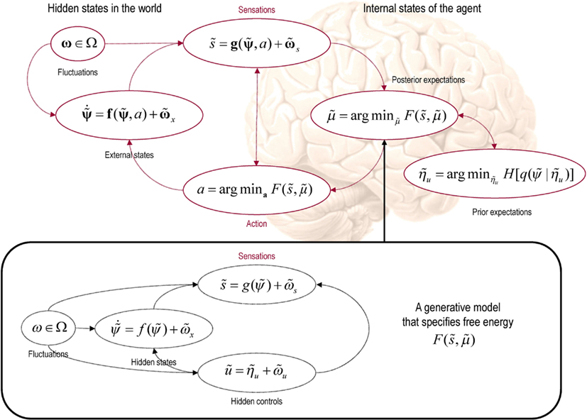
Figure 1. This schematic shows the dependencies among various quantities that are assumed when modeling the exchanges of a self organizing system like the brain with the environment. The top panel describes the states of the environment and the system or agent in terms of a probabilistic dependency graph, where connections denote directed dependencies. The quantities are described within the nodes of this graph with exemplar forms for their dependencies on other variables (see main text). Here, hidden and internal states are separated by action and sensory states. Both action and internal states encoding a conditional density minimize free energy, while internal states encoding prior beliefs maximize salience. Both free energy and salience are defined in terms of a generative model that is shown as fictive dependency graph in the lower panel. Note that the variables in the real world and the form of their dynamics are different from that assumed by the generative model; this is why external states are in bold. Furthermore, note that action is a state in the model of the brain but is replaced by hidden controls in the brain’s model of its world. This means that the agent is not aware of action but has beliefs about hidden causes in the world that action can fulfill through minimizing free energy. These beliefs correspond to prior expectations that sensory states will be sampled in a way that optimizes conditional confidence or salience.

The Infomax Perspective

Priors about hidden controls express the belief that conditional uncertainty will be minimal. The long-term average of this conditional uncertainty is the conditional entropy of hidden states, which can be expressed as the entropy over hidden states minus the mutual information between hidden and sensory states

$H\left(\Psi |S\right)=E_t\left[H\left(\Psi |S=\tilde{s}\left(t\right)\right)\right]=H\left(\Psi \right)-I\left(\Psi ;S\right)$(8)

In other words, minimizing conditional uncertainty is equivalent to maximizing the mutual information between external states and their sensory consequences. This is one instance of the Infomax principle (Linsker, 1990). Previously, we have considered the relationship between free-energy minimization and the principle of maximum mutual information, or minimum redundancy (Barlow, 1961, 1974; Optican and Richmond, 1987; Oja, 1989; Olshausen and Field, 1996; Bialek et al., 2001) in terms of the mapping between hidden and internal states (Friston, 2010). In this setting, one can show that “the Infomax principle is a special case of the free-energy principle that obtains when we discount uncertainty and represent sensory data with point estimates of their causes.” Here, we consider the mapping between external and sensory states and find that prior beliefs about how sensory states are sampled further endorse the Infomax principle.

The Signal Detection Perspective

A related perspective comes from signal detection theory (Morgan, 2011) and the sensitivity of sensory mappings to external states of the world: For a sensory mapping with additive Gaussian noise (in which sensory precision is not state dependent):

$\begin{array}{llll}\tilde{s}& =\tilde{g}\left(\tilde{\psi }\right)+\tilde{\omega }& & \\ p\left(\tilde{\omega }|m\right)& =\mathcal{N }\left(0,{\Sigma }_{\omega }\right)& & \\ p\left(\bar{\psi }|m\right)& =\mathcal{N }\left(\tilde{\eta },{\Sigma }_{\psi }\right)& & \\ G\left(\tilde{s},\tilde{\mu }\right)& =\frac{1}{2}{\left(\tilde{s}-\tilde{g}\left(\tilde{\mu }\right)\right)}^T{\Pi }_{\omega }\left(\tilde{s}-\tilde{g}\left(\tilde{\mu }\right)\right)-\frac{1}{2}ln\left|{\Pi }_{\omega }\right|& & \\ & +\frac{1}{2}{\left(\tilde{\mu }-\tilde{\eta }\right)}^T{\Pi }_{\psi }\left(\tilde{\mu }-\tilde{\eta }\right)& & \\ H\left[q\left(\tilde{\psi }\right)\right]& =-\frac{1}{2}ln\left|{\partial }_{\tilde{\mu }}{\tilde{g}}^T{\Pi }_{\omega }{\partial }_{\tilde{\mu }}\tilde{g}+{\Pi }_{\psi }\right|& & \text{(9)}\end{array}$

This means minimizing conditional uncertainty (as approximated by the entropy of the conditional density) rests on maximizing signal to noise: ${\partial }_{\tilde{\mu }}{\tilde{g}}^T{\prod }_{\omega }{\partial }_{\tilde{\mu }}\tilde{g}.$ Here, the gradients of the sensory mapping ${\partial }_{\tilde{\mu }}\tilde{g}$ can be regarded as the sensitivity of the sensory mapping to changes in hidden states, where this sensitivity depends on hidden controls.

There are several interesting points to be made here: first, when the sensory mapping is linear, its gradient is constant and conditional uncertainty does not depend upon hidden controls. In this instance, everything is equally salient and there are no optimal prior beliefs about hidden controls. This has been the simplifying assumption in previous treatments of the free-energy principle, where “the entropy of hidden states is upper-bounded by the entropy of sensations, assuming their sensitivity to hidden states is constant, over the range of states encountered” (Friston, 2010). However, this assumption fails with sensory mappings that are non-linear in hidden controls. Important examples in the visual domain include visual occlusion, direction of gaze and, most simply, the level of illumination. The last example speaks directly to the dark room problem and illustrates its resolution by prior beliefs: if an agent found itself in a dark room, the simplest way to increase the gain or sensitivity of its sensory mapping would be to switch on a light. This action would be induced by prior beliefs that there will be light, provided the agent has a generative model of the proprioceptive and visual consequences of illuminating the room. Note that action is caused by proprioceptive predictions under beliefs about hidden controls (changes in illumination), which means the agent does not have to know or model how its actions change hidden controls.

Finally, although we will not pursue it in this paper, the conditional entropy or salience also depends on how causes affect sensory precision. This is only relevant when sensory precision is state dependent; however, this may be important in the context of attention and salience. We have previously cast attention has optimizing conditional expectations about precision (Feldman and Friston, 2010). In the current context, this optimization will affect salience and subsequent sensory sampling. This will be pursued in another paper.

The Bayesian Surprise Perspective

Bayesian surprise is a measure of salience based on the Kullback–Leibler divergence between the conditional density (which encodes posterior beliefs) and the prior density (Itti and Baldi, 2009). It measures the information in the data that can be recognized. Empirically, humans direct their gaze toward visual features with high Bayesian surprise: “subjects are strongly attracted toward surprising locations, with 72% of all human gaze shifts directed toward locations more surprising than the average, a figure which rises to 84% when considering only gaze targets simultaneously selected by all subjects” (Itti and Baldi, 2009). In the current setup, Bayesian surprise is the cross entropy or divergence between the posterior and priors over hidden states

$D\left[q\left(\tilde{\psi }\right)\left|\right|p\left(\tilde{\psi }|m\right)\right]=E_q\left\{-lnp\left(\tilde{\psi }|m\right)\right\}-H\left[q\left(\tilde{\psi }\right)\right]$(10)

If prior beliefs about hidden states are uninformative, the first term is roughly constant. This means that maximizing salience is the same as maximizing Bayesian surprise. This is an important observation because it links salience in the context of active inference with the large literature on salience in the theoretical (Humphreys et al., 2009) and empirical (Shen et al., 2011; Wardak et al., 2011) visual sciences; where Bayesian surprise was introduced to explain visual searches in terms of salience.

Minimizing free energy will generally increase Bayesian surprise, because Bayesian surprise is also the complexity cost associated with updating beliefs to explain sensory data more accurately (Friston, 2010). The current arguments suggest that prior beliefs about how we sample the world - to minimize uncertainty about our inferences - maximize Bayesian surprise explicitly. The term Bayesian surprise can be a bit confusing because minimizing surprise per se (or maximizing model evidence) involves keeping Bayesian surprise (complexity) as small as possible. This paradox can be resolved here by noting that agents expect Bayesian surprise to be maximized and then acting to minimize their surprise, given what they expect.

In summary, the imperative to maximize salience or conditional confidence about the causes of sensations emerges naturally from the basic premise that self organizing biological systems (like the brain) minimize the dispersion of their external states when subject to an inconstant and fluctuating environment. This imperative, expressed in terms of prior beliefs about hidden controls in the world that are fulfilled by action, is entirely consistent with the principle of maximum information transfer, sensitivity arguments from signal detection theory and formulations of salience in terms of Bayesian surprise. In what follows, we now consider the neurobiological implementation of free-energy minimization through active inference:

Neurobiological Implementation of Active Inference

In this section, we take the general principles above and consider how they might be implemented in the brain. The equations in this section may appear a bit complicated; however, they are based on just four assumptions:

• The brain minimizes the free energy of sensory inputs defined by a generative model.

• This model includes prior expectations about hidden controls that maximize salience.

• The generative model used by the brain is hierarchical, non-linear, and dynamic.

• Neuronal firing rates encode the expected state of the world, under this model.

The first assumption is the free-energy principle, which leads to active inference in the embodied context of action. The second assumption follows from the arguments of the previous section. The third assumption is motivated easily by noting that the world is both dynamic and non-linear and that hierarchical causal structure emerges inevitably from a separation of temporal scales (Ginzburg and Landau, 1950; Haken, 1983). Finally, the fourth assumption is the Laplace assumption that, in terms of neural codes, leads to the Laplace code that is arguably the simplest and most flexible of all neural codes (Friston, 2009).

Given these assumptions, one can simulate a whole variety of neuronal processes by specifying the particular equations that constitute the brain’s generative model. The resulting perception and action are specified completely by the above assumptions and can be implemented in a biologically plausible way as described below (see Table 1 for a list of previous applications of this scheme). In brief, these simulations use differential equations that minimize the free energy of sensory input using a generalized (gradient) descent (Friston et al., 2010b).

$\begin{array}{l}\dot{\tilde{\mu }}\left(t\right)=\mathrm{𝒟 }\tilde{\mu }\left(t\right)-{\partial }_{\tilde{\mu }}F\left(\tilde{s},\tilde{\mu }\right)\\ \dot{a}\left(t\right)=-{\partial }_{a}F\left(\tilde{s},\tilde{\mu }\right)\end{array}$(11)

TABLE 1

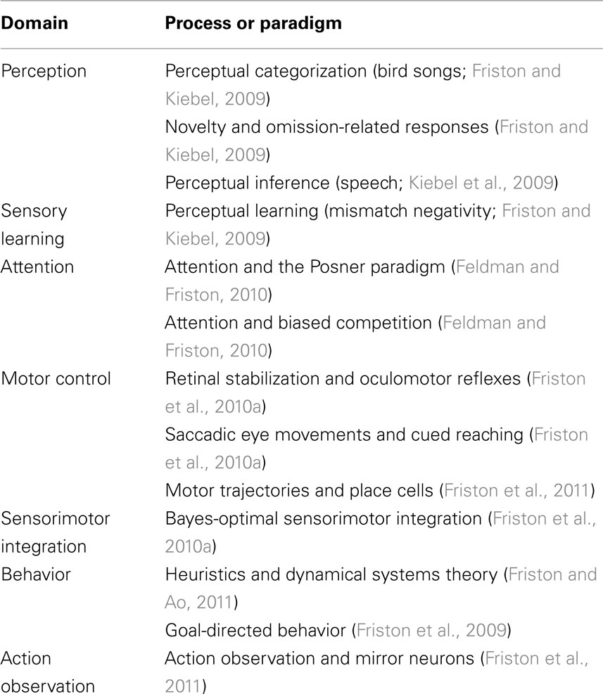
Table 1. Processes and paradigms that have been modeled using the scheme in this paper.

These coupled differential equations describe perception and action respectively and just say that internal brain states and action change in the direction that reduces free energy. The first is known as (generalized) predictive coding and has the same form as Bayesian (e.g., Kalman–Bucy) filters used in time series analysis; see also (Rao and Ballard, 1999). The first term in Eq. 11 is a prediction based upon a differential matrix operator 𝒟 that returns the generalized motion of the expectation, such that $𝒟\tilde{\mu }={\left[{\mu }^{\prime },{\mu }^{″},{\mu }^{‴},\dots \right]}^T.$ The second term is usually expressed as a mixture of prediction errors that ensures the changes in conditional expectations are Bayes-optimal predictions about hidden states of the world. The second differential equation says that action also minimizes free energy - noting that free energy depends on action through sensory states S: Ψ ×A × Ω → ℝ. The differential equations in (11) are coupled because sensory input depends upon action, which depends upon perception through the conditional expectations. This circular dependency leads to a sampling of sensory input that is both predicted and predictable, thereby minimizing free energy and surprise.

To perform neuronal simulations under this framework, it is only necessary to integrate or solve Eq. 11 to simulate the neuronal dynamics that encode conditional expectations and ensuing action. Conditional expectations depend upon the brain’s generative model of the world, which we assume has the following (hierarchical) form

$\begin{array}{c}s=g^{\left(1\right)}\left(x^{\left(1\right)},v^{\left(1\right)},u^{\left(i\right)}\right)+{\omega }_v^{\left(1\right)}\\ {ẋ}^{\left(1\right)}=f^{\left(1\right)}\left(x^{\left(1\right)},v^{\left(1\right)},u^{\left(i\right)}\right)+{\omega }_x^{\left(1\right)}\\ ⋮\\ v^{\left(i-1\right)}=g^{\left(i\right)}\left(x^{\left(i\right)},v^{\left(i\right)},u^{\left(i\right)}\right)+{\omega }_v^{\left(i\right)}\\ {ẋ}^{\left(i\right)}=f^{\left(i\right)}\left(x^{\left(i\right)},v^{\left(i\right)},u^{\left(i\right)}\right)+{\omega }_x^{\left(i\right)}\\ ⋮\end{array}$(12)

This equation is just a way of writing down a model that specifies a probability density over the sensory and hidden states, where the hidden states Ψ = X × V × U have been divided into hidden dynamic, causal and control states. Here [g⁽ⁱ⁾, f ⁽ⁱ⁾] are non-linear functions of hidden states that generate sensory inputs at the first (lowest) level, where, for notational convenience, v⁽⁰⁾: = s.

Hidden causes V ⊂ Ψ can be regarded as functions of hidden dynamic states; hereafter, hidden states X ⊂ Ψ. Random fluctuations $\left({\omega }_x^{\left(i\right)},{\omega }_v^{\left(i\right)}\right)$ on the motion of hidden states and causes are conditionally independent and enter each level of the hierarchy. It is these that make the model probabilistic: they play the role of sensory noise at the first level and induce uncertainty about states at higher levels. The (inverse) amplitudes of these random fluctuations are quantified by their precisions $\left({\prod }_x^{\left(i\right)},{\prod }_v^{\left(i\right)}\right),$ which we assume to be fixed in this paper. Hidden causes link hierarchical levels, whereas hidden states link dynamics over time. Hidden states and causes are abstract quantities (like the motion of an object in the field of view) that the brain uses to explain or predict sensations. In hierarchical models of this sort, the output of one level acts as an input to the next. This input can produce complicated (generalized) convolutions with deep (hierarchical) structure.

Perception and Predictive Coding

Given the form of the generative model (Eq. 12) we can now write down the differential equations (Eq. 11) describing neuronal dynamics in terms of (precision-weighted) prediction errors on the hidden causes and states. These errors represent the difference between conditional expectations and predicted values, under the generative model (using A · B: = A^TB and omitting higher-order terms):

$\begin{array}{l}{\dot{\tilde{\mu }}}_x^{\left(i\right)}=\mathrm{𝒟 }{\tilde{\mu }}_x^{\left(i\right)}+\frac{\partial {\tilde{g}}^{\left(i\right)}}{\partial {\tilde{\mu }}_x^{\left(i\right)}}\cdot {\xi }_v^{\left(i\right)}+\frac{\partial {\tilde{f}}^{\left(i\right)}}{\partial {\tilde{\mu }}_x^{\left(i\right)}}\cdot {\xi }_x^{\left(i\right)}-{\mathrm{𝒟 }}^T{\xi }_x^{\left(i\right)}\\ {\dot{\tilde{\mu }}}_v^{\left(i\right)}=\mathrm{𝒟 }{\tilde{\mu }}_v^{\left(i\right)}+\frac{\partial {\tilde{g}}^{\left(i\right)}}{\partial {\tilde{\mu }}_v^{\left(i\right)}}\cdot {\xi }_v^{\left(i\right)}+\frac{\partial {\tilde{f}}^{{\left(i\right)}^T}}{\partial {\tilde{\mu }}_v^{\left(i\right)}}\cdot {\xi }_x^{\left(i\right)}-{\xi }_v^{\left(i+1\right)}\\ {\dot{\tilde{\mu }}}_u^{\left(i\right)}=\mathrm{𝒟 }{\tilde{\mu }}_u^{\left(i\right)}+\frac{\partial {\tilde{g}}^{\left(i\right)}}{\partial {\tilde{\mu }}_u^{\left(i\right)}}\cdot {\xi }_v^{\left(i\right)}+\frac{\partial {\tilde{f}}^{\left(i\right)}}{\partial {\tilde{\mu }}_u^{\left(i\right)}}\cdot {\xi }_x^{\left(i\right)}-{\xi }_u^{\left(i+1\right)}\\ {\xi }_x^{\left(i\right)}={\prod }_x^{\left(i\right)}\left(\mathrm{𝒟 }{\tilde{\mu }}_x^{\left(i\right)}-{\tilde{f}}^{\left(i\right)}\left({\tilde{\mu }}_x^{\left(i\right)},{\tilde{\mu }}_v^{\left(i\right)},{\tilde{\mu }}_u^{\left(i\right)}\right)\right)\\ {\xi }_v^{\left(i\right)}={\prod }_v^{\left(i\right)}\left({\tilde{\mu }}_v^{\left(i-1\right)}-{\tilde{g}}^{\left(i\right)}\left({\tilde{\mu }}_x^{\left(i\right)},{\tilde{\mu }}_v^{\left(i\right)},{\tilde{\mu }}_u^{\left(i\right)}\right)\right)\\ {\xi }_u^{\left(i\right)}={\prod }_u^{\left(i\right)}\left({\tilde{\mu }}_v^{\left(i-1\right)}-{\tilde{\eta }}_u^{\left(i\right)}\right)\end{array}$(13)

Equation 13 can be derived fairly easily by computing the free energy for the hierarchical model in Eq. 12 and inserting its gradients into Eq. 11. What we end up with is a relatively simple update scheme, in which conditional expectations are driven by a mixture of prediction errors, where prediction errors are defined by the equations of the generative model.

It is difficult to overstate the generality and importance of Eq. 13: its solutions grandfather nearly every known statistical estimation scheme, under parametric assumptions about additive or multiplicative noise (Friston, 2008). These range from ordinary least squares to advanced variational deconvolution schemes. The resulting scheme is called generalized filtering or predictive coding (Friston et al., 2010b). In neural network terms, Eq. 13 says that error units receive predictions from the same level and the level above. Conversely, conditional expectations (encoded by the activity of state units) are driven by prediction errors from the same level and the level below. These constitute bottom-up and lateral messages that drive conditional expectations toward a better prediction to reduce the prediction error in the level below. This is the essence of recurrent message passing between hierarchical levels to optimize free energy or suppress prediction error: see Friston and Kiebel (2009) for a more detailed discussion. In neurobiological implementations of this scheme, the sources of bottom-up prediction errors, in the cortex, are thought to be superficial pyramidal cells that send forward connections to higher cortical areas. Conversely, predictions are conveyed from deep pyramidal cells, by backward connections, to target (polysynaptically) the superficial pyramidal cells encoding prediction error (Mumford, 1992; Friston and Kiebel, 2009). Figure 2 provides a schematic of the proposed message passing among hierarchically deployed cortical areas.

FIGURE 2

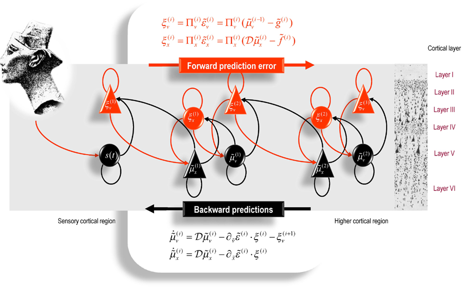
Figure 2. Schematic detailing the neuronal architecture that might encode conditional expectations about the states of a hierarchical model. This shows the speculative cells of origin of forward driving connections that convey prediction error from a lower area to a higher area and the backward connections that construct predictions (Mumford, 1992). These predictions try to explain away prediction error in lower levels. In this scheme, the sources of forward and backward connections are superficial and deep pyramidal cells respectively. The equations represent a generalized descent on free-energy under the hierarchical models described in the main text: see also (Friston, 2008). State units are in black and error units in red. Here, neuronal populations are deployed hierarchically within three cortical areas (or macro-columns). Within each area, the cells are shown in relation to cortical layers: supra-granular (I–III) granular (IV) and infra-granular (V–VI) layers. For simplicity, conditional expectations about control states had been absorbed into conditional expectations about hidden causes.

Action

In active inference, conditional expectations elicit behavior by sending top-down predictions down the hierarchy that are unpacked into proprioceptive predictions at the level of the cranial nerve nuclei and spinal-cord. These engage classical reflex arcs to suppress proprioceptive prediction errors and produce the predicted motor trajectory

$ȧ=-\frac{\partial }{\partial a}F=-\frac{\partial \tilde{s}}{\partial a}\cdot {\xi }_v^{\left(1\right)}$(14)

The reduction of action to classical reflexes follows because the only way that action can minimize free energy is to change sensory (proprioceptive) prediction errors by changing sensory signals; cf., the equilibrium point formulation of motor control (Feldman and Levin 1995). In short, active inference can be regarded as equipping a generalized predictive coding scheme with classical reflex arcs: see (Friston et al., 2009, 2010a) for details. The actual movements produced clearly depend upon top-down predictions that can have a rich and complex structure, due to perceptual optimization based on the sampling of salient exteroceptive and interoceptive inputs.

Counterfactual Processing

To optimize prior expectations about hidden controls it is necessary to identify those that maximize the salience of counterfactual representations implicit in the counterfactual density in Eq. 7. Clearly, there are many ways this could be implemented. In this paper, we will focus on visual searches and assume that counterfactual expectations are represented explicitly and place coded in a saliency map over the space of hidden causes. In other words, we will assume that salience is encoded on a grid corresponding to discrete values of counterfactual expectations associated with different hidden control states. The maximum of this map defines the counterfactual expectation with the greatest salience, which then becomes the prior expectation about hidden control states. This prior expectation enters the predictive coding in Eq. 13. The salience of the j-th counterfactual expectation is, from Eqs 9 and 12,

$\begin{array}{l}{\tilde{\eta }}_u\left(t\right)=arg{max}_{{\tilde{\eta }}_j}S\left({\tilde{\eta }}_j\right)\\ S\left({\tilde{\eta }}_j\right)=-H\left[q\left(\tilde{\psi }|{\tilde{\mu }}_x\left(t+\tau \right),{\tilde{\mu }}_v\left(t+\tau \right),{\tilde{\eta }}_j\right)\right]\\ =\frac{1}{2}ln\left|{\partial }_{\tilde{\psi }}{\tilde{\epsilon }}_j^T{\Pi }_{\omega }{\partial }_{\tilde{\psi }}{\tilde{\epsilon }}_j+{\Pi }_{\psi }\right|\end{array}$(15)

where the counterfactual prediction errors and their precisions are:

$\begin{array}{l}{\widetilde{𝒟}}_j^{\left(i\right)}=\left[\begin{array}{c}𝒟{\tilde{\mu }}_x^{\left(i\right)}-{\tilde{f}}^{\left(i\right)}\left({\tilde{\mu }}_x^{\left(i\right)},{\tilde{\mu }}_v^{\left(i\right)},{\tilde{\eta }}_j^{\left(i\right)}\right)\\ {\tilde{\mu }}_v^{\left(i-1\right)}-{\tilde{g}}^{\left(i\right)}\left({\tilde{\mu }}_x^{\left(i\right)},{\tilde{\mu }}_v^{\left(i\right)},{\tilde{\eta }}_j^{\left(i\right)}\right)\\ {\tilde{\mu }}_u^{\left(i-1\right)}-{\tilde{\eta }}_u^{\left(i\right)}\end{array}\right],\\ {\prod }_{\omega }^{\left(i\right)}=\left[\begin{array}{ccc}{\prod }_x^{\left(i\right)}& & \\ & {\prod }_v^{\left(i\right)}& \\ & & {\prod }_u^{\left(i\right)}\end{array}\right]\\ {\tilde{\epsilon }}_j=\left[\begin{array}{c}{\epsilon }_j^{\left(1\right)}\\ ⋮\\ {\epsilon }_j^{\left(n\right)}\end{array}\right],{\prod }_{\omega }=\left[\begin{array}{ccc}{\prod }_{\omega }^{\left(1\right)}& & \\ & \ddots & \\ & & {\prod }_{\omega }^{\left(n\right)}\end{array}\right]\end{array}$(16)

Given that we will be simulating visual searches with saccadic eye movements, we will consider the prior expectations to be updated at discrete times to simulate successive saccades, where the hidden controls correspond to locations in the visual scene that attract visual fixation.

Summary

In summary, we have derived equations for the dynamics of perception and action using a free-energy formulation of adaptive (Bayes-optimal) exchanges with the world and a generative model that is both generic and biologically plausible. In what follows, we use Eqs 13–15 to simulate neuronal and behavioral responses. A technical treatment of the material above can be found in (Friston et al., 2010a), which provides the details of the scheme used to integrate Eq. 11 to produce the simulations in the next section. The only addition to previous illustrations of this scheme is Eq. 15, which maps conditional expectations about hidden states to prior expectations about hidden controls: it is this mapping that underwrites the sampling of salient features and appeals to the existence of hidden control states that action can change. Put simply, this formulation says that action fulfills predictions and we predict that the consequences of action (i.e., hidden controls) minimize the uncertainty about predictions.

Modeling Saccadic Eye Movements

In this section, we will illustrate the theory of the previous section, using simulations of sequential eye movements. Saccadic eye movements are a useful vehicle to illustrate active inference about salient features of the world because they speak directly to visual search strategies and a wealth of psychophysical, neurobiological, and theoretical study (e.g., Grossberg et al., 1997; Ferreira et al., 2008; Srihasam et al., 2009; Bisley and Goldberg, 2010; Shires et al., 2010; Tatler et al., 2011; Wurtz et al., 2011). Having said this, we do not aim to provide detailed neurobiological simulations of oculomotor control, rather to use the basic phenomenology of saccadic eye movements to illustrate the key features of the optimal inference scheme described above. This scheme can be regarded as a formal example of active vision (Wurtz et al., 2011); sometimes described in enactivist terms as visual palpation (O’Regan and Noë, 2001).

In what follows, we describe the production of visual signals and how they are modeled in terms of a generative model. We will focus on a fairly simple paradigm – the categorization of faces – and therefore sidestep many of the deeper challenges of understanding visual searches. These simulations should not be taken as a serious or quantitative model of saccadic eye movements – they just represent a proof of principle to illustrate the basic phenomenology implied by prior beliefs that constitute a generative model. Specifying a generative model allows us to compute the salience of stimulus features that are sampled and enables us to solve or integrate Eq. 11 to simulate the neuronal encoding of posterior beliefs and ensuing action. We will illustrate this in terms of oculomotor dynamics and the perception of a visual stimulus or scene. The simulations reported below can be reproduced by calling (annotated) Matlab scripts from the DEM graphical user interface (Visual search), available as academic freeware (http://www.fil.ion.ucl.ac.uk/spm/).

The Generative Process

To integrate the generalized descent on free energy in Eq. 11, we need to define the processes generating sensory signals as a function of (hidden) states and action:

$\begin{array}{l}{s}_p={\text{x}}_p+{\omega }_{v,p}\\ s_q=g\left(I,{\text{x}}_p\right)+{\omega }_{v,q}\\ g_i=I\left(d_{i,1}+{\text{x}}_{p,1},d_{i,2}+{\text{x}}_{p,2}\right).h_i\\ {\dot{\text{x}}}_p=a-\frac{1}{16}{x}_p+{\omega }_{x,p}\end{array}$(17)

Note that these hidden states are true states that actually produce sensory signals. These have been written in boldface to distinguish them from the hidden states assumed by the generative model (see below). In these simulations, the world is actually very simple: sensory signals are generated in two modalities – proprioception and vision. Proprioception, s_p ∈ ℝ² reports the center of gaze or foveation as a displacement from the origin of some extrinsic frame of reference. Inputs in the visual modality comprise a list s_q ∈ ℝ²⁵⁶ of values over an array of sensory channels sampling a two-dimensional image or visual scene I: ℝ² → ℝ. This sampling uses a grid of 16 × 16 channels that uniformly samples a small part the image (one sixth of the vertical and horizontal extent). The numerical size of the grid was chosen largely for computational expedience. In terms of its size in retinotopic space – it represents a local high-resolution (foveal) sampling that constitutes an attentional focus. To make this sampling more biologically realistic, each channel is equipped with a center-surround receptive field that samples a local weighted average of the image. The weights correspond to a Gaussian function with a standard deviation of one pixel minus another Gaussian function with a standard deviation of four pixels. This provides an on-off center-surround sampling. Furthermore, the signals are modulated by a two-dimensional Hamming function – to model the loss of precise visual information from the periphery of the visual field. This modulation was meant to model the increasing size of classical receptive fields and an attentional down-weighting of visual input with increasing eccentricity from the center of gaze (Feldman and Friston, 2010).

The only hidden states in this generative process x _p ∈ ℝ² are the center of oculomotor fixation, whose motion is driven by action and decays with a suitably long time constant of 16 time bins (each time bin corresponds to 12 ms). These hidden states are also subject to random fluctuations, with a temporal smoothness of one half of a time bin (6 ms). The hidden states determine where the visual scene is sampled (foveated). In practice, the visual scene corresponds to a large grayscale image, where the i-th visual channel is sampled at location d_i + x _p ∈ ℝ² using sinc interpolation (as implemented in the SPM image analysis package). Here, d_i ∈ ℝ² specifies the displacement of the i-th channel from the center of the sampling grid. The proprioceptive and visual signals were effectively noiseless, where there random fluctuations (ω_v,p, ω_v,q) had a log precision of 16. The motion of the fixation point was subject to low amplitude fluctuations (ω_x,p) with a log precision of eight. This completes our description of the process generating proprioceptive and visual signals, for any given visual scene and action-dependent trajectory of hidden states (center of fixation). We now turn to the model of this process that generates predictions and action:

The Generative Model

The model of sensory signals used to specify variational free energy and consequent action (visual sampling) is slightly more complicated than the actual process of generating data:

$\begin{array}{l}{s}_p=x_p+{\omega }_{v,p}\\ s_q=\sum _{i}exp\left(x_{q,i}\right)g\left(I_i,x_p\right)+{\omega }_{v,q}\\ {ẋ}_p=\frac{1}{4}\left(u-x_p\right)+{\omega }_{x,p}\\ {ẋ}_q=1-\sum _{i}exp\left(x_{q,i}\right)-\frac{1}{1024}{x}_q+{\omega }_{x,p}\end{array}$(18)

As in the generative process above, proprioceptive signals are just a noisy mapping from hidden proprioceptive states encoding the direction of gaze. The visual input is modeled as a mixture of images sampled at a location specified by the proprioceptive hidden state. This hidden state decays with a time constant of four time bins (48 ms) toward a hidden control state. In other words, the hidden control determines the location that attracts gaze.

The visual input depends on a number of hypotheses or internal images I_i: ℝ² → ℝ: i ∈ {1,…, N} that constitute the agent’s prior beliefs about what could cause its visual input. In this paper, we use N = 3 hypotheses. The input encountered at any particular time is a weighted mixture of these internal images, where the weights correspond to hidden perceptual states. The dynamics of these perceptual states (last equality above) implement a form of dynamic softmax, in the sense that the solution of their equations of motion ensures the weights sum (approximately) to one:

${ẋ}_q=0\Rightarrow \sum _{i}exp\left(x_{q,i}\right)\approx 1$(19)

This means we can interpret exp(x_q,i) as the (softmax) probability that the i-th internal image or hypothesis is the cause of visual input. The decay term (with a time constant of 512 time bins) just ensures that perceptual states decay slowly to the same value, in the absence of perceptual fluctuations.

In summary, given hidden proprioceptive and perceptual states the agent can predict the proprioceptive and visual input. The generative model is specified by Eq. 18 and the precision of the random fluctuations that determine the agent’s prior certainty about sensory inputs and the motion of hidden states. In the examples below, we used a log precision of eight for proprioceptive sensations and the motion of hidden states that - and let the agent believe its visual input was fairly noisy, with a log precision of four. In practice, this means it is more likely to change its (less precise) posterior beliefs about the causes of visual input to reduce prediction error, as opposing to adjusting its (precise) posterior beliefs about where it is looking. All that now remains is to specify prior beliefs about the hidden control state attracting the center of gaze:

Priors and Saliency

To simulate saccadic eye movements, we integrated the active inference scheme for 16 time bins (196 ms) and then computed a map of salience to reset the prior expectations about the hidden control states that attract the center of gaze. This was repeated eight times to give a sequence of eight saccadic eye movements. The simulation of each saccade involves integrating the coupled differential Eqs 11, 14, and 17 to solve for the true hidden states, action, and posterior expectations encoded by neuronal activity. The integration used a local linearization scheme (Ozaki, 1992) in generalized coordinates of motion as described in several previous publications (Friston et al., 2010a).

The salience was computed for 1024 = 32 × 32 locations distributed uniformly over the visual image or scene. The prior expectation of the hidden control state was the (generalized) location ${\tilde{\eta }}_j\in {\left[{\eta }_j,0,0,\dots \right]}^T$ that maximized salience, according to Eq. 15:

$\begin{array}{c}{\tilde{\eta }}_u=arg\underset{{\tilde{\eta }}_j}{max}S\left({\tilde{\eta }}_j\right)\\ S\left({\tilde{\eta }}_j\right)=-H\left[q\left(\tilde{\psi }|{\tilde{\mu }}_x\left(t+\tau \right),{\tilde{\mu }}_v\left(t+\tau \right),{\tilde{\eta }}_j\right)\right]\end{array}$(20)

The fictive prediction errors at each location where evaluated at their solution under the generative model; namely,

${\tilde{\mu }}_x\left(t+\tau \right)=\left[\begin{array}{c}{\tilde{\mu }}_{x,p}\left(t+\tau \right)={\tilde{\eta }}_j\\ {\tilde{\mu }}_{x,q}\left(t+\tau \right)={\tilde{\mu }}_{x,q}\left(t\right)\end{array}\right]$(21)

In other words, salience is evaluated for proprioceptive and perceptual expectations encoding current posterior beliefs about the content of the visual scene and the fictive point of fixation to which gaze is attracted. The ensuing salience over the 32 × 32 locations constitutes a salience map that drives the next saccade. Notice that salience is a function of, and only of, fictive beliefs about the state of the world and essentially tells the agent where to sample (look) next. Salience depends only on sensory signals vicariously, through the current posterior beliefs. This is important because it means that salience is not an attribute of sensations, but beliefs about those sensations. In other words, salience is an attribute of features we believe to be present in the world and changes with the way that those features are sampled. In the present setting, salience is a function of where the agent looks. Note that the simulations of saccadic eye movements in this paper are slightly unusual, in that the salience map extends beyond the field of view. This means salient locations in the visual scene are represented outside the field of view: these locations are parts of a scene that should provide confirmatory evidence for current hypotheses about the extended (visual) environment.

Figure 3 provides a simple illustration of salience based upon the posterior beliefs or hypothesis that local (foveal) visual inputs are caused by an image of Nefertiti. The left panels summarize the classic results of Yarbus (1967); in terms of a stimulus and the eye movements it elicits. The right panels depict visual input after sampling the image on the right with center-surround receptive fields and the associated saliency map based on a local sampling of 16 × 16 pixels, using Eq. 20. Note how the receptive fields suppress absolute levels of luminance contrast and highlight edges. It is these edges that inform posterior beliefs about both the content of the visual scene and where it is being sampled. This information reduces conditional uncertainty and is therefore salient. The salient features of the image include the ear, eye, and mouth. The location of these features and a number of other salient locations appear to be consistent with the locations that attract saccadic eye movements (as shown on the right). Crucially, the map of salience extends well beyond the field of view (circle on the picture). As noted above, this reflects the fact that salience is not an attribute of what is seen, but what might be seen under a particular hypothesis about the causes of sensations.

FIGURE 3

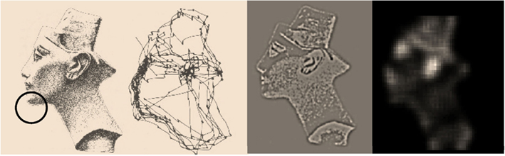
Figure 3. This provides a simple illustration of salience based upon the posterior beliefs or hypothesis that local (foveal) visual inputs are caused by an image of Nefertiti. The left panels summarize the classic results of Yarbus; in terms of a stimulus and the eye movements it elicits. The right panels depict visual input after sampling the image on the right (using conventional center-surround receptive fields) and the associated saliency map based on a local sampling of 16 × 16 pixels, using the generative model described in the main text. The size of the resulting field of view, in relation to the visual scene, is indicated with the circle on the left image. The key thing to note here is that the salient features of the image include the ear, eye, and mouth. The location of these features and other salient locations appear to be consistent with the locations that attract saccadic eye movements (as shown on the left).

To make the simulations a bit more realistic, we added a further prior implementing inhibition of return (Itti and Koch, 2001; Wang and Klein, 2010). This involved suppressing the salience of locations that have been recently foveated, using the following scheme:

$\begin{array}{l}{\mathbf{\text{S}}}_k=S_k-\left(S_k\times R_{k-1}\right)\\ R_k=\rho \left({\mathbf{\text{S}}}_k\right)+\frac{1}{2}{R}_{k-1}\end{array}$(22)

Here, $S_k=S\left({\tilde{\eta }}_j\right)-min\left(S\left({\tilde{\eta }}_j\right)\right)$ is the differential salience for the k-th saccade and R_k is an inhibition of return map that remembers recently foveated locations. This map reduces the salience of previous locations if they were visited recently. The function ρ(S_k) ∈ [0,1] is a Gaussian function (with a standard deviation of 1/16 of the image size) of the distance from the location of maximum salience that attracts the k-th saccade. The addition of inhibition of return ensures that a new location is selected by each saccade and can be motivated ethologically by prior beliefs that the visual scene will change and that previous locations should be revisited.

Functional Anatomy

Figure 4 provides an intuition as to how active inference under salience priors might be implemented in the brain. This schematic depicts a particular instance of the message passing scheme in Figure 2, based on the generative model above. This model prescribes a particular hierarchical form for generalized predictive coding; shown here in terms of state and error units (black and red, denoting deep and superficial pyramidal cell populations respectively) that have been assigned to different cortical or subcortical regions. The insert on the left shows a visual scene (a picture of Nefertiti) that can be sampled locally by foveating a particular point – the true hidden state of the world. The resulting visual input arrives in primary visual cortex to elicit prediction errors that are passed forward to “what” and “where” streams (Ungerleider and Mishkin, 1982). State units in the “what” stream respond by adjusting their representations to provide better predictions based upon a discrete number of internal images or hypotheses. Crucially, the predictions of visual input depend upon posterior beliefs about the direction of gaze, encoded by the state units in the “where” stream (Bisley and Goldberg, 2010). These posterior expectations are themselves informed by top-down prior beliefs about the direction of gaze that maximizes salience. The salience map shown in the center is updated between saccades based upon conditional expectations about the content of the visual scene. Conditional beliefs about the direction of gaze provide proprioceptive predictions to the oculomotor system in the superior colliculus and pontine nuclei, to elaborate a proprioceptive prediction error (Grossberg et al., 1997; Shires et al., 2010; Shen et al., 2011). This prediction error drives the oculomotor system to fulfill posterior beliefs about where to look next. This can be regarded as an instance of the classical reflects arc, whose set point is determined by top-down proprioceptive predictions. The anatomical designations should not be taken seriously (for example, the salience map may be assembled in the pulvinar or frontal cortex and mapped to the deep layer of the superior colliculus). The important thing to take from this schematic is the functional logic implied by the anatomy that involves reciprocal message passing and nested loops in a hierarchical architecture that is not dissimilar to circuits in the real brain. In particular, note that representations of hidden perceptual states provide bilateral top-down projections to early visual systems (to predict visual input) and to the systems computing salience, which might involve the pulvinar of the thalamus (Wardak et al., 2011; Wurtz et al., 2011).

FIGURE 4

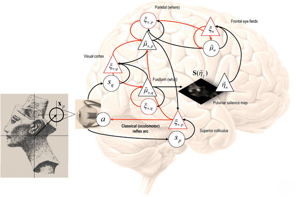
Figure 4. This schematic depicts a particular instance of the message passing scheme in Figure 2. This example follows from the generative model of visual input described in the main text. The model prescribes a particular hierarchical form for generalized predictive coding; shown here in terms of state and error units (black and red respectively) that have been assigned to different cortical or subcortical regions. The insert on the left shows a visual scene (a picture of Nefertiti) that can be sampled locally by foveating a particular point – the true hidden state of the world. The resulting visual input arrives in primary visual cortex to elicit prediction errors that are passed forward to what and where streams. State units in the “what” stream respond by adjusting their representations to provide better predictions based upon a discrete number of internal images or hypotheses. Crucially, the predictions of visual input depend upon posterior beliefs about the direction of gaze encoded by state units in the “where” stream. These conditional expectations are themselves informed by top-down prior beliefs about the direction of gaze that maximizes salience. The salience map shown in the center is updated between saccades based upon posterior beliefs about the content of the visual scene. Posterior beliefs about the content of the visual scene provide predictions of visual input and future hidden states subtending salience. Posterior beliefs about the direction of gaze are used to form predictions of visual input and provide proprioceptive predictions to the oculomotor system in the superior colliculus and pontine nuclei, to elaborate a proprioceptive prediction error. This prediction error drives the oculomotor system to fulfill posterior beliefs about where to look next. This can be regarded as an instance of the classical reflects arc, whose set point is determined by top-down proprioceptive predictions. The variables associated with each region are described in detail in the text, while the arrows connecting regions adopt same format as in Figure 2 (forward prediction error afferents in red and backward predictions in black).

Summary

In this section, we have described the process generating sensory information in terms of a visual scene and hidden states that specify how that scene is sampled. We have described both the likelihood and priors that together comprise a generative model. The special consideration here is that these priors reflect prior beliefs that the agent will sample salient sensory features based upon its current posterior beliefs about the causes of those features. We are now in a position to look at the sorts of behavior this model produces.

Simulating Saccadic Eye Movements

In this section, we present a few examples of visual search under the generative model described above. Our purpose here is to illustrate the nature of active inference, when it is equipped with priors that maximize salience or minimize uncertainty. We will present three simulations; first a canonical simulation in which the visual scene matches one of three internal images or hypotheses. This simulation illustrates the operation of optimal visual searches that select the hypothesis with the lowest free energy and minimize conditional uncertainty about this hypothesis. We will then repeat the simulation using a visual scene that the agent has not experienced and has no internal image of. This is used to illustrate a failure to select a hypothesis and the consequent itinerant sampling of the scene. Finally, largely for fun, we simulate a “dark room” agent whose prior beliefs compel it to sample the least salient locations to demonstrate how these priors result in sensory seclusion from the environment.

Figure 5 shows the results of the first simulation, in which the agent had three internal images or hypotheses about the scene it might sample (an upright face, an inverted face, and a rotated face). The agent was presented with an upright face and its posterior expectations were evaluated over 16 (12 ms) time bins, after which salience was evaluated. The agent then emitted a saccade by foveating the most salient location during the subsequent 16 time bins – from its starting location (the center of the visual field). This was repeated for eight saccades. The upper row shows the ensuing eye movements as red dots (in the extrinsic coordinates of the true scene) at the fixation point of each saccade. The corresponding sequence of eye movements is shown in the insert on the upper left, where the red circles correspond roughly to the agent’s field of view. These saccades were driven by prior beliefs about the direction of gaze based upon the salience maps in the second row. Note that these maps change with successive saccades as posterior beliefs about the hidden perceptual states become progressively more confident. Note also that salience is depleted in locations that were foveated in the previous saccade – this reflects the inhibition of return. Posterior beliefs about hidden states provide visual and proprioceptive predictions that suppress visual prediction errors and drive eye movements respectively. Oculomotor responses are shown in the third row in terms of the two hidden oculomotor states corresponding to vertical and horizontal displacements. The portions of the image sampled (at the end of each saccade) are shown in the fourth row (weighted by the Hamming function above). The final two rows show the posterior beliefs in terms of their sufficient statistics (penultimate row) and the perceptual categories (last row) respectively. The posterior beliefs are plotted here in terms of posterior expectations and 90% confidence interval about the true stimulus. The key thing to note here is that the expectation about the true stimulus supervenes over its competing representations and, as a result, posterior confidence about the stimulus category increases (the posterior confidence intervals shrink to the expectation): see (Churchland et al., 2011) for an empirical study of this sort phenomena. The images in the lower row depict the hypothesis selected; their intensity has been scaled to reflect conditional uncertainty, using the entropy (average uncertainty) of the softmax probabilities.

FIGURE 5

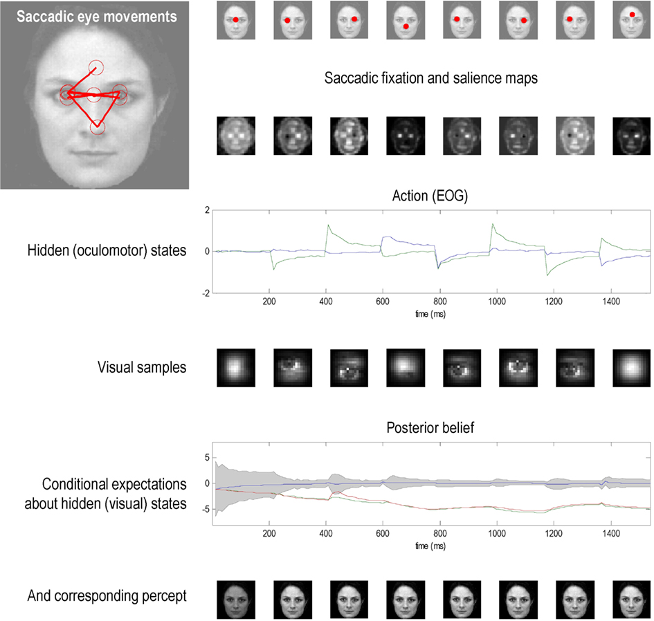
Figure 5. This figure shows the results of the first simulation, in which a face was presented to an agent, whose responses were simulated using the optimal inference scheme described in the main text. In this simulation, the agent had three internal images or hypotheses about the stimuli it might sample (an upright face, an inverted face, and a rotated face). The agent was presented with an upright face and its conditional expectations were evaluated over 16 (12 ms) time bins until the next saccade was emitted. This was repeated for eight saccades. The ensuing eye movements are shown as red dots at the location (in extrinsic coordinates) at the end of each saccade in the upper row. The corresponding sequence of eye movements is shown in the insert on the upper left, where the red circles correspond roughly to the proportion of the image sampled. These saccades are driven by prior beliefs about the direction of gaze based upon the saliency maps in the second row. Note that these maps change with successive saccades as posterior beliefs about the hidden states, including the stimulus, become progressively more confident. Note also that salience is depleted in locations that were foveated in the previous saccade. These posterior beliefs provide both visual and proprioceptive predictions that suppress visual prediction errors and drive eye movements respectively. Oculomotor responses are shown in the third row in terms of the two hidden oculomotor states corresponding to vertical and horizontal displacements. The associated portions of the image sampled (at the end of each saccade) are shown in the fourth row. The final two rows show the posterior beliefs in terms of their sufficient statistics and the stimulus categories respectively. The posterior beliefs are plotted here in terms of conditional expectations and the 90% confidence interval about the true stimulus. The key thing to note here is that the expectation about the true stimulus supervenes over its competing expectations and, as a result, conditional confidence about the stimulus category increases (the confidence intervals shrink to the expectation). This illustrates the nature of evidence accumulation when selecting a hypothesis or percept that best explains sensory data. Within-saccade accumulation is evident even during the initial fixation with further stepwise decreases in uncertainty as salient information is sampled at successive saccades.

This simulation illustrates a number of key points. First, it illustrates the nature of evidence accumulation in selecting a hypothesis or percept the best explains sensory data. One can see that this proceeds over two timescales; both within and between saccades. Within-saccade accumulation is evident even during the initial fixation, with further stepwise decreases in uncertainty as salient information is sampled. The within-saccade accumulation is formally related to evidence accumulation as described in models of perceptual discrimination (Gold and Shadlen, 2003; Churchland et al., 2011). This is meant in the sense that the posterior expectations about perceptual states are driven by prediction errors. However, the accumulation here rests explicitly on the formal priors implied by the generative model. In this case, the prevalence of any particular perceptual category is modeled as a dynamical process that has certain continuity properties. In other words, inherent in the model is the belief that the content of the world changes in a continuous fashion. This means that posterior beliefs have a persistence or slower timescale than would be observed under schemes that just accumulate evidence. This is reflected in the progressive elevation of the correct perceptual state above its competitors and the consequent shrinking of the posterior confidence interval. The transient changes in the posterior beliefs, shortly after each saccade, reflect the fact that new data are being generated as the eye sweeps toward its new target location. It is important to note that the agent is not just predicting visual contrast, but also how contrast changes with eye movements – this induces an increase in conditional uncertainty (in generalized coordinates of motion) during the fast phase of the saccade. However, due to the veracity of the posterior beliefs, the conditional confidence shrinks again when the saccade reaches its target location. This shrinkage is usually to a smaller level than in the previous saccade.

This illustrates the second key point; namely, the circular causality that lies behind perception. Put simply, the only hypothesis that can endure over successive saccades is the one that correctly predicts the salient features that are sampled. This sampling depends upon action or an embodied inference that speaks directly to the notion of visual palpation (sniffing; O’Regan and Noë, 2001). This means that the hypothesis prescribes its own verification and can only survive if it is a correct representation of the world. If its salient features are not discovered, it will be discarded in favor of a better hypothesis. This provides a nice perspective on perception as hypothesis testing, where the emphasis is on the selective processes that underlie sequential testing. This is particularly pertinent when hypotheses can make predictions that are more extensive than the data available at any one time.

Finally, although the majority of saccades target the eyes and nose, as one might expect, there is one saccade to the forehead. This is somewhat paradoxical, because the forehead contains no edges and cannot increase posterior confidence about a face. However, this region is highly informative under the remaining two hypotheses (corresponding to the location of the nose in the inverted face and the left eye in the rotated face). This subliminal salience is revealed through inhibition of return and reflects the fact that the two competing hypotheses have not been completely excluded. This illustrates the competitive nature of perceptual selection induced by inhibition of return and can regarded, heuristically, as occasional checking of alternative hypotheses. This is a bit like a scientist who tries to refute his hypothesis by acquiring data that furnish efficient tests of his competing or null hypotheses.

We then repeated the simulation, but used an unknown (unrecognizable) face – the image of Nefertiti from previous Figures. Because the agent has no internal image or hypothesis that can produce veridical predictions about salient locations to foveate, it cannot resolve the causes of its sensory input and is unable to assimilate visual information into a precise posterior belief. (See Figure 6). Saccadic movements are generated by a saliency map that represents the most salient locations based upon a mixture of all internal hypotheses about the stimulus. The salience maps here have a lower spatial resolution than in the previous figure because sensory channels are deployed over a larger image. Irrespective of where the agent looks, it can find no posterior beliefs or hypothesis that can explain the sensory input. As a result, there is a persistent conditional uncertainty about the states of the world that fail to resolve themselves. The ensuing percepts are poorly formed and change sporadically with successive saccades.

FIGURE 6

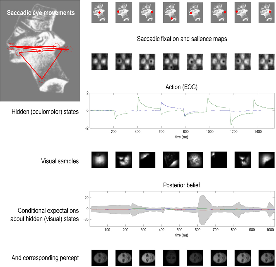
Figure 6. This figure uses the same format as the previous figure, but shows the result of presenting an unknown (unrecognizable) face – the image of Nefertiti from previous figures. Because the agent has no internal image or hypothesis that can produce veridical predictions about salient locations to foveate, it cannot resolve the causes of its sensory input and is unable to assimilate visual information into a precise posterior belief about the stimulus. Saccadic movements are generated by a saliency map that represents the most salient locations based upon a mixture of all internal hypotheses about the stimulus. Irrespective of where the agent looks, it can find no posterior beliefs or hypothesis that can explain the sensory input. As a result, there is a persistent posterior uncertainty about the states of the world that fail to resolve themselves. The ensuing percepts are poorly formed and change sporadically with successive saccades.

Finally, we presented a known (recognizable) face to an agent whose prior beliefs minimize salience, as opposed to maximize it. This can be regarded as an agent that (a priori) prefers dark rooms. This agent immediately foveates the least informative part of the scene and maintains fixation at that location – see Figure 7. This results in a progressive increase in uncertainty and ambiguity about the stimulus causing visual input; as reflected in the convergence of posterior expectations about the three hypotheses and an increase in conditional uncertainty (penultimate row). As time progresses, the percept fades (lower row) and the agent is effectively sequestered from its sensorium. Note here how the salience map remains largely unchanged and encodes a composite salience of all (three) prior hypotheses about visual input.

FIGURE 7

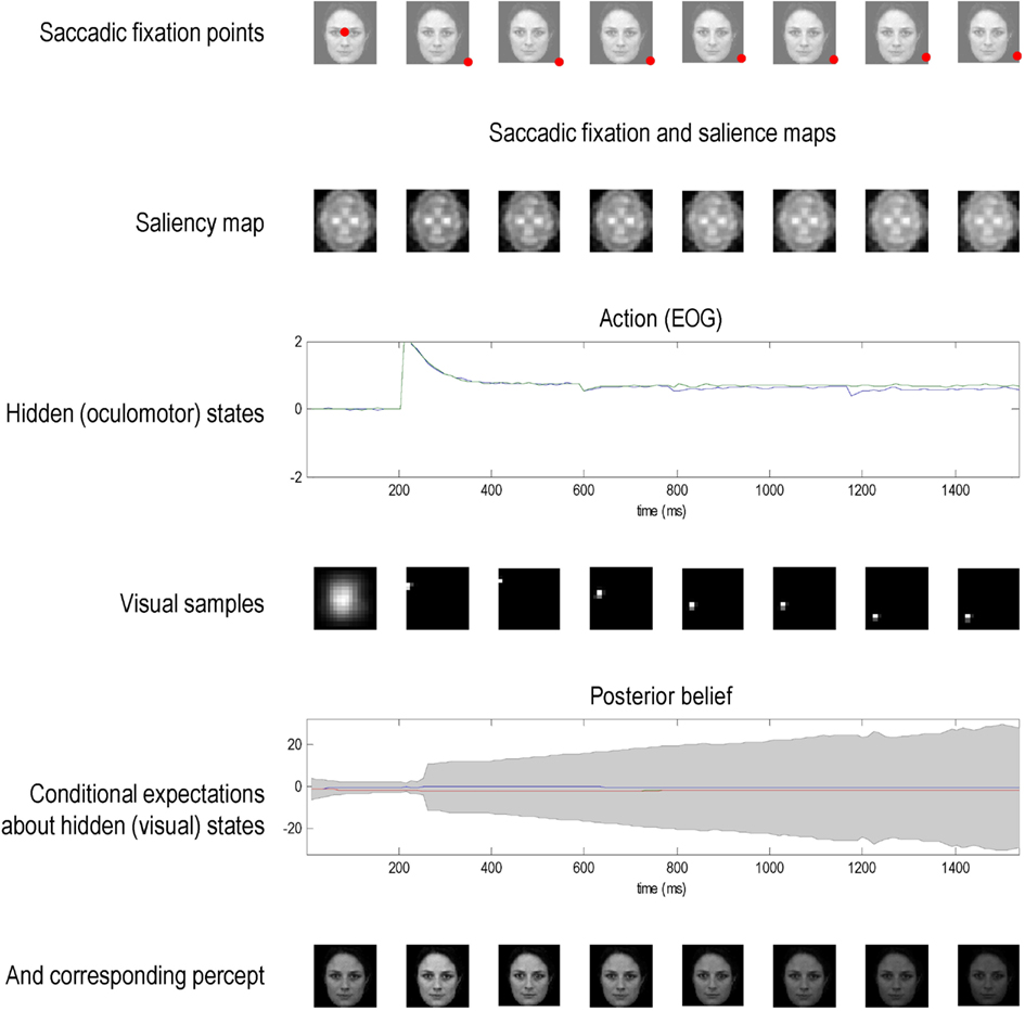
Figure 7. This figure uses the same format as the previous figures but shows the result of presenting a known (recognizable) face to an agent whose prior beliefs about eye movements are that they should minimize salience, as opposed to maximize it. This can be regarded as an agent that prefers dark rooms. This agent immediately foveates the least informative part of the scene and maintains fixation at that location (because the inhibition of return operates by decreasing the salience of the location foveated previously). This results in a progressive increase in uncertainty about the stimulus; as reflected in the convergence of posterior expectations about the three hypotheses and an increase in conditional uncertainty (penultimate row). As time progresses, the percept fades (lower row) and the agent is effectively sequestered from its sensorium. Note here how the salience map remains largely unchanged and encodes a composite salience of all (three) prior hypotheses about states of the world causing visual input.

Discussion

This work suggests that we can understand exploration of the sensorium in terms of optimality principles based on straightforward ergodic or homoeostatic principles. In other words, to maintain the constancy of our external milieu, it is sufficient to expose ourselves to predicted and predictable stimuli. Being able to predict what is currently seen also enables us to predict fictive sensations that we could experience from another viewpoint. The mathematical arguments presented in the first section suggest that the best viewpoint is the one that confirms our predictions with the greatest precision or certainty. In short, action fulfills our predictions, while we predict the consequences of our actions will maximize confidence in those predictions. This provides a principled way in which to explore and sample the world; for example, with visual searches using saccadic eye movements. These theoretical considerations are remarkably consistent with a number of compelling heuristics; most notably the Infomax principle or the principle of minimum redundancy, signal detection theory, and recent formulations of salience in terms of Bayesian surprise.

Simulations of successive saccadic eye movements or visual search, based on maximizing saliency or posterior precision reproduce, in a phenomenological sense, some characteristics of visual searches seen empirically. Although these simulations should not be taken as serious proposals for the neurobiology of oculomotor control, they do provide a rough proof of principle for the basic idea. An interesting perspective on perception emerges from the simulations, in which percepts are selected through a form of circular causality: in other words, only the correct percept can survive the cycle of action and perception, when the percept is used to predict where to look next. If the true state of the world and the current hypothesis concur, then the percept can maintain itself by selectively sampling evidence for its own existence. This provides an embodied (enactivist) explanation for perception that fits comfortably with the notion of visual sniffing or palpation (O’Regan and Noë, 2001; Wurtz et al., 2011), in contrast to passive evidence accumulation schemes. Having said this, evidence accumulation is an integral part of optimal inference; in the sense that dynamics on representations of hidden states, representing competing hypotheses, are driven by prediction errors. However, this is only part of the story; in that emerging representations come to play a role in determining where to search for evidence. This is illustrated nicely in the context of saccadic eye movements of the sort we have simulated.

There are many limitations of the current scheme that we have glossed over. For example, there is no principled reason why we should include inhibition of return. Of course, we can appeal to natural selection to say that this sort of prior belief would be more robust in a changing environment; however, this sort of proposition is best substantiated with simulations or analytic arguments. The question here would be whether inhibition of return is an emergent property of free-energy minimization or Bayes-optimal sampling of the visual scene. Another simplifying assumption that we have made is that the agent executes a new saccade or search on a fixed and slow timescale, without considering how saccadic eye movements are actually triggered or when they may be triggered in an optimal fashion (Grossberg et al., 1997). Note that the emission of sporadic movements follows from the sporadic updates of the salience map – the actual movement is responding continuously to proprioceptive predictions based upon salience. One advantage of considering sporadic updates is that the solution of fictive hidden states in the future becomes relatively simple; for example, given prior beliefs about hidden control (the location of a point attractor of foveation), it is a relatively simple matter to compute the hidden states in the future (that are attracted to that location). This advantage may have been exploited by evolution. However, the fixed timescale (16 times bins of 12 ms) does not account for the link between when and where in oculomotor control – observed particularly in reading studies (Rayner, 1978): Solving for fictive states in the future may not be simple when hidden causes are changing quickly – as in reading (Yarbus, 1967). Eye movements have been studied extensively in the context of reading or have been used to infer reading processes. Huge amounts of data are available (including corpus studies) and it would be interesting to see how the current framework could explain robust effects in reading. Moreover, models of oculomotor control in reading – such as EZ-Reader or SWIFT (Rayner, 2009) – are particularly elaborate and include contextual constraints (allowing predictions) and mechanisms linking where and when decisions. These schemes represent interesting task-specific models that may lend themselves to integration in the theoretical framework introduced here. Finally, we have not paid much attention to the vast amount of work on the neurobiology of saccadic eye movements and their functional anatomy. It will be an interesting exercise to see how much of the empirical work on the psychophysics and neurophysiology of saccades can be addressed using the theory above.

There are a number of obvious next steps that suggest themselves. For example, endowing the generative model with a deeper hierarchical structure and allowing it to represent multiple objects at the same time. One can see, at least intuitively, how the ensuing inference would correspond to scene construction and require one to address fundamental issues like translational invariance and the representation of things like occlusion and depth. The hierarchical nature of representations is particularly interesting from the point of view of face processing: for example Miellet et al. (2011) showed that observers can use either a local (sampling foveal information) or a global (sampling diagnostic extra-foveal features) strategy – suggesting “that face identification is not rooted in a single, or even preferred, information-gathering strategy” (Miellet et al., 2011). In the same vein, a central fixation bias has been established for Eastern observers (Blais et al., 2008; Miellet et al., 2010). The nature of hierarchical inference may be crucial for a formal understanding of these phenomena: in hierarchical generative models, hidden causes are represented at multiple levels of abstraction, each with conditional dependencies on other levels. This means that each – global or local – level contributes to conditional uncertainty and will therefore compete in determining the most salient sensory samples that resolve uncertainty. One can see how a context-sensitive competition among different levels of representation could manifest as a switching between the sampling of sensory information that informs local and global features (Miellet et al., 2011). In principle, this sort of competition could be simulated by repeating the simulations presented above, using a hierarchical generative model.

It would also be interesting to simulate bistable perception within the current framework, using ambiguous figures and binocular presentation. The illustrations in this paper have used static visual scenes; however, the same principles could be applied to dynamically changing scenes and should, hopefully, reproduce the sorts of saccades seen in reading. The solutions to hidden fictive states in this dynamic context would be more complicated but not computationally intractable. Finally, we have not considered microsaccadic or fixation or movements. In the setting of active inference, fast microscopic movements represent an interesting area of study because they are the product closed loop feedback control with multiple hierarchically deployed loops (see Figure 4). This suggests that their statistics should show some interesting features characteristic of self-organized dynamics that are not bound to a particular temporal scale. We look forward to addressing these and other theoretical issues.

As noted by our reviewers, not all sensory epithelia can be moved around to search the sensorium – as in active touch and vision. For example, how could we generalize this approach to audition? An intriguing possibility is the prior beliefs that guide the active sampling of somatosensory and visual information could also guide directed attention. In Feldman and Friston (2010), we described the use of prior beliefs – about the location of precise sensory information – to explain the behavioral and electrophysiological correlates of attention (in the context of the Posner paradigm and biased competition). One might imagine that prior beliefs about the location of salient sensory information would not just inform proprioceptive predictions but predictions about the precision of sensory signals at particular locations in visual and auditory space. Turning this conjecture around, it suggests that (directed) attention could be understood – and implemented – in terms of prior beliefs about salient sensory channels that provide precise sensory confirmation of latent perceptual hypotheses. This perspective may provide a nice (formal) unification of overt active searches and covert attentional searches, in terms of prior beliefs that select where we look and where we attend.

It should be noted that the contribution of this work is purely conceptual and that we have not considered any empirical validation of the underlying ideas. There are many theoretically informed empirical initiatives that touch on the issues we have considered and much more: see Thurtell et al. (2011), Dandekar et al. (2012), Morvan and Maloney (2012), Purcell et al. (2012) for recent examples. There are a number of interesting ways in which the computational ideas above could be linked to empirical studies of saccadic eye movements. First, one could focus on empirically derived salience maps and try to reverse engineer the underlying visual hypotheses that subjects were entertaining. In other words, Eq. 15 provides a model of a salience map – in terms of underlying hypothetical images and precisions; which (in principle) can be estimated, given an empirical salience map based on occupancy during visual searches. One could take this a stage further and use the simulations above as a generative or forward model of real eye movements – in terms of their statistics as measured with eye tracking or in terms of neuronal responses measured with electroencephalography. The exciting thing here is that one could then optimize the model parameters (e.g., internal templates) or compare different models of salience using Bayesian model comparison. As noted by one of our reviewers, the (neuronally plausible) predictive coding scheme we used to simulate saccadic eye movements can also be used to simulate event related potentials. This speaks to the interesting notion of modeling eye movements measured with eye tracking, oculomotor responses with electrooculography, and event related neuronal responses with electroencephalography. In principle, this modeling could furnish a dynamic causal model (David et al., 2006) of multimodal responses – elicited by visual searches – that is both physiologically and computationally informed. This is outstanding but potentially important work that could provide empirical evidence for the theoretical ideas presented in this and other papers.

In summary, we have tried to formalize the intuitive notion that are interactions with the world are akin to sensory experiments, by which we confirm our hypotheses about its causal structure in an optimal and efficient fashion. This mandates prior beliefs that the deployment of sensory epithelia and our physical relationship to the world will disclose its secrets – beliefs that are fulfilled by action. The resulting active or embodied inference means that not only can we regard perception as hypotheses, but we could regard action as performing experiments that confirm or disconfirm those hypotheses.

Conflict of Interest Statement

The authors declare that the research was conducted in the absence of any commercial or financial relationships that could be construed as a potential conflict of interest.

Acknowledgments

This work was funded by the Wellcome trust. We would like to thank our reviewers for very helpful guidance on how to present and contextualize this work. Laurent Perrinet was supported by European Union project Number FP7-269921, “Brain-Scales” and project “CODDE” from Seventh Framework Program FP7/2007-2013 under agreement number 214728-2.

References

Ashby, W. R. (1947). Principles of the self-organizing dynamic system. J. Gen. Psychol. 37, 125–128.

Pubmed Abstract | Pubmed Full Text | CrossRef Full Text

Ballard, D. H., Hinton, G. E., and Sejnowski, T. J. (1983). Parallel visual computation. Nature 306, 21–26.

Pubmed Abstract | Pubmed Full Text | CrossRef Full Text

Barlow, H. (1961). “Possible principles underlying the transformations of sensory messages,” in Sensory Communication, ed. W. Rosenblith (Cambridge, MA: MIT Press), 217–34.

Barlow, H. B. (1974). Inductive inference, coding, perception, and language. Perception 3, 123–134.

Pubmed Abstract | Pubmed Full Text | CrossRef Full Text

Beal, M. J. (2003). Variational Algorithms for Approximate Bayesian Inference. Ph.D. thesis, University College London, London.

Bialek, W., Nemenman, I., and Tishby, N. (2001). Predictability, complexity, and learning. Neural Comput. 13, 2409–2463.

Pubmed Abstract | Pubmed Full Text | CrossRef Full Text

Bisley, J. W., and Goldberg, M. E. (2010). Attention, intention, and priority in the parietal lobe. Annu. Rev. Neurosci. 33, 1–21.

Pubmed Abstract | Pubmed Full Text | CrossRef Full Text

Blais, C., Jack, R. E., Scheepers, C., Fiset, D., and Caldara, R. (2008). Culture shapes how we look at faces. PLoS ONE 3, e3022. doi:10.1371/journal.pone.0003022

CrossRef Full Text

Churchland, A. K., Kiani, R., Chaudhuri, R., Wang, X. J., Pouget, A., and Shadlen, M. N. (2011). Variance as a signature of neural computations during decision making. Neuron 69, 818–831.

Pubmed Abstract | Pubmed Full Text | CrossRef Full Text

Dandekar, S., Privitera, C., Carney, T., and Klein, S. A. (2012). Neural saccadic response estimation during natural viewing. J. Neurophysiol. 107, 1776–1790.

Pubmed Abstract | Pubmed Full Text | CrossRef Full Text

Daunizeau, J., Preuschoff, K., Friston, K., and Stephan, K. (2011). Optimizing experimental design for comparing models of brain function. PLoS Comput Biol. 7, e1002280. doi:10.1371/journal.pcbi.1002280

CrossRef Full Text

David, O., Kiebel, S., Harrison, L., Mattout, J., Kilner, J. M., and Friston, K. J. (2006). Dynamic causal modeling of evoked responses in EEG and MEG. Neuroimage 30, 1255–1272.

Pubmed Abstract | Pubmed Full Text | CrossRef Full Text

Dayan, P., Hinton, G. E., and Neal, R. (1995). The Helmholtz machine. Neural Comput. 7, 889–904.

Pubmed Abstract | Pubmed Full Text | CrossRef Full Text

Feldman, A. G., and Levin, M. F. (1995). The origin and use of positional frames of reference in motor control. Behav. Brain Sci. 18, 723–806.

CrossRef Full Text

Feldman, H., and Friston, K. J. (2010). Attention, uncertainty, and free-energy. Front. Hum. Neurosci. 4:215. doi:10.3389/fnhum.2010.00215

CrossRef Full Text

Ferreira, F., Apel, J., and Henderson, J. M. (2008). Taking a new look at looking at nothing. Trends Cogn. Sci. (Regul. Ed.) 12, 405–410.

Pubmed Abstract | Pubmed Full Text | CrossRef Full Text

Feynman, R. P. (1972). Statistical Mechanics. Reading, MA: Benjamin.

Friston, K. (2005). A theory of cortical responses. Philos. Trans. R. Soc. Lond. B. Biol. Sci. 360, 815–836.

Pubmed Abstract | Pubmed Full Text | CrossRef Full Text

Friston, K. (2008). Hierarchical models in the brain. PLoS Comput. Biol. 4, e1000211. doi:10.1371/journal.pcbi.1000211

CrossRef Full Text

Friston, K. (2009). The free-energy principle: a rough guide to the brain? Trends Cogn. Sci. (Regul. Ed.) 13, 293–301.

Pubmed Abstract | Pubmed Full Text | CrossRef Full Text

Friston, K. (2010). The free-energy principle: a unified brain theory? Nat. Rev. Neurosci. 11, 127–138.

Pubmed Abstract | Pubmed Full Text | CrossRef Full Text

Friston, K., and Ao, P. (2011). Free-energy, value and attractors. Comput. Math. Methods Med. 2012, doi:10.1155/2012/937860

Pubmed Abstract | Pubmed Full Text | CrossRef Full Text

Friston, K., Thornton, C., and Clark, A. (2012). Free-energy minimization and the dark-room problem. Front. Psychol. 3:130. doi:10.3389/fpsyg.2012.00130

CrossRef Full Text

Friston, K., and Kiebel, S. (2009). Cortical circuits for perceptual inference. Neural Netw. 22, 1093–1104.

Pubmed Abstract | Pubmed Full Text | CrossRef Full Text

Friston, K., Kilner, J., and Harrison, L. (2006). A free energy principle for the brain. J. Physiol. Paris 100, 70–87.

Pubmed Abstract | Pubmed Full Text | CrossRef Full Text

Friston, K., Mattout, J., and Kilner, J. (2011). Action understanding and active inference. Biol. Cybern. 104, 137–160.

Pubmed Abstract | Pubmed Full Text | CrossRef Full Text

Friston, K. J., Daunizeau, J., and Kiebel, S. J. (2009). Active inference or reinforcement learning? PLoS ONE 4, e6421. doi:10.1371/journal.pone.0006421

Pubmed Abstract | Pubmed Full Text | CrossRef Full Text

Friston, K. J., Daunizeau, J., Kilner, J., and Kiebel, S. J. (2010a). Action and behavior: a free-energy formulation. Biol. Cybern. 102, 227–260.

CrossRef Full Text

Friston, K., Stephan, K., Li, B., and Daunizeau, J. (2010b). Generalised Filtering. Math. Probl. Eng. 2010, 621670.

CrossRef Full Text

Gibson, J. J. (1979). The Ecological Approach to Visual Perception. Boston: Houghton Mifflin.

Ginzburg, V. L., and Landau, L. D. (1950). On the theory of superconductivity. Zh. Eksp. Teor. Fiz. 20, 1064.

Gold, J. I., and Shadlen, M. N. (2003). The influence of behavioral context on the representation of a perceptual decision in developing oculomotor commands. J. Neurosci. 23, 632–651.

Pubmed Abstract | Pubmed Full Text

Gregory, R. L. (1980). Perceptions as hypotheses. Philos. Trans. R. Soc. Lond. B Biol. Sci. 290, 181–197.

Pubmed Abstract | Pubmed Full Text | CrossRef Full Text

Grossberg, S., Roberts, K., Aguilar, M., and Bullock, D. (1997). A neural model of multimodal adaptive saccadic eye movement control by superior colliculus. J. Neurosci. 17, 9706–9725.

Pubmed Abstract | Pubmed Full Text

Haken, H. (1983). Synergetics: An Introduction. Non-Equilibrium Phase Transition and Self-Selforganisation in Physics, Chemistry and Biology, 3rd Edn. Berlin: Springer Verlag.

Helmholtz, H. (1866/1962). “Concerning the perceptions in general,” in Treatise on Physiological Optics, 3rd Edn, Vol. III, ed. J. Southall, trans. (New York: Dover).

Humphreys, G. W., Allen, H. A., and Mavritsaki, E. (2009). Using biologically plausible neural models to specify the functional and neural mechanisms of visual search. Prog. Brain Res. 176, 135–148.

Pubmed Abstract | Pubmed Full Text

Itti, L., and Baldi, P. (2009). Bayesian surprise attracts human attention. Vision Res. 49, 1295–1306.

Pubmed Abstract | Pubmed Full Text | CrossRef Full Text

Itti, L., and Koch, C. (2001). Computational modelling of visual attention. Nat. Rev. Neurosci. 2, 194–203.

Pubmed Abstract | Pubmed Full Text | CrossRef Full Text

Jaynes, E. T. (1957). Information theory and statistical mechanics. Phys. Rev. 106, 620–630.

CrossRef Full Text

Kiebel, S. J., Daunizeau, J., and Friston, K. J. (2009). Perception and hierarchical dynamics. Front. Neuroinform. 3:20. doi:10.3389/neuro.11.020.2009

CrossRef Full Text

Knill, D. C., and Pouget, A. (2004). The Bayesian brain: the role of uncertainty in neural coding and computation. Trends Neurosci. 27, 712–719.

Pubmed Abstract | Pubmed Full Text | CrossRef Full Text

Linsker, R. (1990). Perceptual neural organization: some approaches based on network models and information theory. Annu. Rev. Neurosci. 13, 257–281.

Pubmed Abstract | Pubmed Full Text | CrossRef Full Text

Miellet, S., Caldara, R., and Schyns, P. G. (2011). Local Jekyll and global Hyde: the dual identity of face identification. Psychol. Sci. 22, 1518–1526.

Pubmed Abstract | Pubmed Full Text | CrossRef Full Text

Miellet, S., Zhou, X., He, L., Rodger, H., and Caldara, R. (2010). Investigating cultural diversity for extrafoveal information use in visual scenes. J. Vis. 10, 21.

Pubmed Abstract | Pubmed Full Text | CrossRef Full Text

Morgan, M. J. (2011). Features and the ‘primal sketch.’ Vision Res. 51, 738–753.

Pubmed Abstract | Pubmed Full Text | CrossRef Full Text

Morvan, C., and Maloney, L. T. (2012). Human visual search does not maximize the post-saccadic probability of identifying targets. PLoS Comput. Biol. 8, e1002342. doi:10.1371/journal.pcbi.1002342

CrossRef Full Text

Mumford, D. (1992). On the computational architecture of the neocortex. II. Biol. Cybern. 66, 241–251.

Pubmed Abstract | Pubmed Full Text | CrossRef Full Text

Oja, E. (1989). Neural networks, principal components, and subspaces. Int. J. Neural Syst. 1, 61–68.

CrossRef Full Text

Olshausen, B. A., and Field, D. J. (1996). Emergence of simple-cell receptive field properties by learning a sparse code for natural images. Nature 381, 607–609.

Pubmed Abstract | Pubmed Full Text | CrossRef Full Text

Optican, L., and Richmond, B. J. (1987). Temporal encoding of two-dimensional patterns by single units in primate inferior cortex. II Information theoretic analysis. J. Neurophysiol. 57, 132–146.

Pubmed Abstract | Pubmed Full Text

O’Regan, J. K., and Noë, A. (2001). A sensorimotor account of vision and visual consciousness. Behav. Brain Sci. 24, 939–973.

Pubmed Abstract | Pubmed Full Text | CrossRef Full Text

Ozaki, T. (1992). A bridge between nonlinear time-series models and stochastic dynamical systems: a local linearization approach. Stat. Sin. 2, 113–135.

Purcell, B. A., Schall, J. D., Logan, G. D., and Palmeri, T. J. (2012). From salience to saccades: multiple-alternative gated stochastic accumulator model of visual search. J. Neurosci. 32, 3433–3446.

Pubmed Abstract | Pubmed Full Text | CrossRef Full Text

Rao, R. P., and Ballard, D. H. (1999). Predictive coding in the visual cortex: a functional interpretation of some extra-classical receptive-field effects. Nat. Neurosci. 2, 79–87.

Pubmed Abstract | Pubmed Full Text | CrossRef Full Text

Rayner, K. (1978). Eye movements in reading and information processing. Psychol. Bull. 85, 618–660.

Pubmed Abstract | Pubmed Full Text | CrossRef Full Text

Rayner, K. (2009). Eye movements in reading: models and data. J. Eye Mov. Res. 2, 1–10.

Pubmed Abstract | Pubmed Full Text

Shen, K., Valero, J., Day, G. S., and Paré, M. (2011). Investigating the role of the superior colliculus in active vision with the visual search paradigm. Eur. J. Neurosci. 33, 2003–2016.

Pubmed Abstract | Pubmed Full Text | CrossRef Full Text

Shires, J., Joshi, S., and Basso, M. A. (2010). Shedding new light on the role of the basal ganglia-superior colliculus pathway in eye movements. Curr. Opin. Neurobiol. 20, 717–725.

Pubmed Abstract | Pubmed Full Text | CrossRef Full Text

Srihasam, K., Bullock, D., and Grossberg, S. (2009). Target selection by the frontal cortex during coordinated saccadic and smooth pursuit eye movements. J. Cogn. Neurosci. 21, 1611–1627.

Pubmed Abstract | Pubmed Full Text | CrossRef Full Text

Tatler, B. W., Hayhoe, M. M., Land, M. F., and Ballard, D. H. (2011). Eye guidance in natural vision: reinterpreting salience. J. Vis. 11, 5.

Pubmed Abstract | Pubmed Full Text | CrossRef Full Text

Thurtell, M. J., Joshi, A. C., Leigh, R. J., and Walker, M. F. (2011). Three-dimensional kinematics of saccadic eye movements in humans: is the “half-angle rule” obeyed? Ann. N. Y. Acad. Sci. 1233, 34–40.

Pubmed Abstract | Pubmed Full Text | CrossRef Full Text

Ungerleider, L. G., and Mishkin, M. (1982). “Two cortical visual systems,” in Analysis of Visual Behavior, eds D. Ingle, M. A. Goodale, and R. J. Mansfield (Cambridge, MA: MIT Press), 549–586.

Wang, Z., and Klein, R. M. (2010). Searching for inhibition of return in visual search: a review. Vision Res. 50, 220–228.

Pubmed Abstract | Pubmed Full Text | CrossRef Full Text

Wardak, C., Olivier, E., and Duhamel, J. R. (2011). The relationship between spatial attention and saccades in the frontoparietal network of the monkey. Eur. J. Neurosci. 33, 1973–1981.

Pubmed Abstract | Pubmed Full Text | CrossRef Full Text

Wurtz, R. H., McAlonan, K., Cavanaugh, J., and Berman, R. A. (2011). Thalamic pathways for active vision. Trends Cogn. Sci. (Regul. Ed.) 5, 177–184.

CrossRef Full Text

Yarbus, A. L. (1967). Eye Movements and Vision. New York: Plenum.

Yuille, A., and Kersten, D. (2006). Vision as Bayesian inference: analysis by synthesis? Trends Cogn. Sci. (Regul. Ed.) 10, 301–308.

Pubmed Abstract | Pubmed Full Text | CrossRef Full Text