The 2N-ary Choice Tree Model for N-Alternative Preferential Choice

The 2N-ary choice tree model accounts for response times and choice probabilities in multi-alternative preferential choice. It implements pairwise comparison of alternatives on weighted attributes into an information sampling process which, in turn, results in a preference process. The model provides expected choice probabilities and response time distributions in closed form for optional and fixed stopping times. The theoretical background of the 2N-ary choice tree model is explained in detail with focus on the transition probabilities that take into account constituents of human preferences such as expectations, emotions, or socially influenced attention. Then it is shown how the model accounts for several context-effects observed in human preferential choice like similarity, attraction, and compromise effects and how long it takes, on average, for the decision. The model is extended to deal with more than three choice alternatives. A short discussion on how the 2N-ary choice tree model differs from the multi-alternative decision field theory and the leaky competing accumulator model is provided.

1. Introduction

Life is full of decisions: Be it the selection of clothing in the morning or of menu for lunch, the question which car to buy or if taking cold medication is necessary. This type of decisions is called preferential choice and has been subject of numerous investigations within the field of decision theory (Koehler and Harvey, 2007, for a review). Several effects have been observed when the decision maker has more than two-choice options (multi-alternative preferential choice). Hick’s Law (Hick, 1952; Hyman, 1953), originally defined in the context of stimulus detection paradigms, postulates a dependency of deliberation time on the number of alternatives. In particular, it states that a linear increase of the number of equally attractive alternatives to choose from leads to a logarithmic increase of the time that passes until the decision is made. Furthermore, a decision maker who is indifferent between two-choice alternatives from a given choice set may change the preference for one or the other alternative when the choice set is enlarged, i.e., the local context may affect the decision and generate preference reversals. Similarity effects (Tversky, 1972), attraction effects (Huber et al., 1982), and compromise effects (Simonson, 1989), for instance, depend on a third alternative that is added to a choice set of two equally attractive but dissimilar alternatives. If the third alternative is very similar to one of the others, the two similar alternatives share their choice frequency and are both chosen less often than the dissimilar one (similarity effect). If the third alternative is similar to one of the others but slightly inferior, it promotes the similar one and increases its choice frequency compared to the dissimilar one (attraction effect). If the third alternative is a compromise between the other two, the decision maker will prefer the compromise to the other alternatives (compromise effect). Besides those preference reversals that emerge from local context, there might also be influence from background context (Tversky and Simonson, 1993) like a reference point outside of the choice set which – together with the loss-aversion principle (Kahneman and Tversky, 1979) – affects evaluation of the given alternatives.

One challenge for (cognitive) modelers is to think of a model which predicts decision making behavior for multi-alternative preferential choice tasks in general but also accounts for all the aforementioned effects. Another challenge is to formulate the model such that (expected) response times and choice probabilities can be calculated and the model parameters conveniently estimated from the observed choice times and choice frequencies.

Decision field theory (DFT, Busemeyer and Townsend, 1992, 1993) and its multi-attribute extension (Diederich, 1997) predict choice response times and choice probabilities for binary choice tasks. Both approaches provide closed form solutions to calculate these entities. Since then, several attempts have been made to extend this kind of models to multi-alternative preferential choice tasks: multi-alternative DFT (Roe et al., 2001) and the leaky competing accumulator (LCA) model (Usher and McClelland, 2001, 2004) predict choice probabilities for three alternative choice tasks but cannot account for optional choice times, i.e., the time the decision maker needs to come to a decision. Both approaches, however, do account for fixed stopping times, i.e., for an externally determined time limit. Furthermore, multi-alternative DFT and the LCA model both account for the similarity, attraction, and compromise effects using computer simulations to predict the patterns. To do so Roe et al. (2001) interpret DFT as a connectionist network and implement distance-dependent inhibition between the alternatives. Usher and McClelland(2001, 2004) add insights from perceptual choice and neuropsychology to the multi-alternative DFT and propose for their LCA model direct implementation of loss-aversion by means of an asymmetric value function and global inhibition instead of distance-dependent inhibition.

Our 2N-ary choice tree model builds on the previous approaches and tries to overcome some of their problems. It is a general model for choice probabilities and response times in choice between N alternatives with D attributes. As such, it provides a way to calculate expected response times, response time distributions, and choice probabilities in closed form by determining the time course of an information sampling process via a random walk on a specific tree. It is able to account for similarity, attraction, and compromise effects which have been most challenging for previous models. In contrast to previous approaches, the 2N-ary choice tree model accounts for these effects without additional mechanisms like inhibition or loss-aversion and is thus more parsimonious. However, it is possible to implement these mechanisms if the situation requires it.

First, we describe the structure of the 2N-ary choice tree and the implementation of the random walk on it in general, including a discussion of initial values and stopping rules. Then we define expected choice probabilities and reaction times and state that these exist and can be calculated in finite time. The proof of this statement is given later in the paper. It is not essential for understanding the theory; we provide it rather as completing the theoretical derivations. Next, we show how to derive transition probabilities from the given alternatives in a specific choice set and therewith define the random walk for that set. A psychological interpretation of their constituents is given afterward. Finally, we demonstrate the predictive power of our model by showing several simulations for choice situations producing the similarity, attraction, and compromise effect and calculate expected hitting times and choice probabilities. We conclude with a comparison of the 2N-ary choice tree with its closest competitors, the multi-alternative DFT and the LCA model.

2. The 2N-ary Choice Tree Model

Making an informed decision usually implies sampling of information about the alternatives under consideration. In Psychology, information sampling processes (e.g., Townsend and Ashby, 1983; Luce, 1986, for review, LaBerge, 1962; Laming, 1968; Link and Heath, 1975; Townsend and Ashby, 1983; Luce, 1986; Ratcliff and Smith, 2004) have a long tradition and proven to be an adequate tool for detailed interpretation of decision making processes, mostly in perception as they provide insight about accuracy and time course of these processes. Poisson counter models (e.g., Pike, 1966; Townsend and Ashby, 1983; LaBerge, 1994; Diederich, 1995; Smith and Van Zandt, 2000; Van Zandt et al., 2000) are a special class of information sampling models that assume constant amounts of information being sampled at Poisson distributed points in time. (Multi-alternative) DFT (Busemeyer and Townsend, 1993; Roe et al., 2001) and the LCA model (Usher and McClelland, 2004) make use of information sampling principles in modeling preferential choice under uncertainty. Both models assume one counter per alternative and all of these counters are updated once per fixed time interval until one of them reaches a threshold. The amounts to update the counters depend on comparison of the alternatives and on already sampled information. In our 2N-ary choice tree model, only one counter per fixed time interval is updated with a fixed amount, but the probability for each counter to be updated depends on comparison of the alternatives and on already sampled information. With regard to its constituents it is thus based on the same principles as both DFT and the LCA model. As only one counter is updated per iteration, the next time for a specific counter to be updated depends on the given probabilities. Hence the technical component of the 2N-ary choice tree model resembles a counter model.

2.1. 2N-ary Choice Trees

In contrast to the aforementioned models, the 2N-ary choice tree model assigns two counters to each of N alternatives in a given choice set. One of them samples positive information, i.e., information in favor of the respective alternative, the other one samples negative information, i.e., information against it. Their difference describes the actual preference state relating to that alternative. As an example, consider two alternatives A and B. The four counters are labeled A⁺, A⁻, B⁺, and B⁻ and yield the preference states Pref(A) = A⁺ − A⁻ for alternative A and Pref(B) = B⁺ − B⁻ for alternative B. Beginning at a fixed point in time, the model chooses one counter and increases its state by one whenever a specific time interval h (e.g., 1 ms) has passed. The length h of the time interval can be chosen arbitrarily with a shorter time interval leading to more precision in the calculation of expected choice probabilities and choice response times. Due to limitations of recording devices, experimental data will be discrete as well and it is thus not necessary to aim for a continuous model. Note that increasing only one counter state at a time with a fixed amount of evidence equal to one is equivalent to increasing all counter states at the same time with an amount of evidence equal to the probability with which these counters are chosen and which also sum up to one (see below). Updating counters at discrete points in time creates a discrete structure of possible combinations of counter states which can be interpreted as graph or, more precisely, as (b-ary) tree¹.

Definition 1 (b-ary tree): A b-ary tree is a rooted tree T = (V, E, r) with vertices V, edges E ⊆ V × V and root r ∈ V where all vertices are directed away from r and each internal vertex has b children.

For N choice alternatives, consider a 2N-ary tree T = (V, E, r). Figure 1 depicts the 4-ary tree for the two-alternative example. The topmost vertex is the root r with outgoing edges directing to four vertices that represent the counters A⁺, A⁻, B⁺, and B⁻. Each of these vertices has four outgoing edges and thus four children itself, and so forth. The information sampling process is mapped to this tree as a walk, i.e., a sequence of edges and vertices, beginning with the root r that takes one step, i.e., passes from one vertex through an edge to another vertex, per time interval h. Whenever the walk reaches a vertex, the counter with the same label is updated by + 1. Figure 2 shows an example for a walk on the 4-ary tree where first counter B⁺ (information in favor of choice alternative B), then counter A⁻ (unfavorable information for choosing alternative A) and then again counter B⁺ is updated.

FIGURE 1

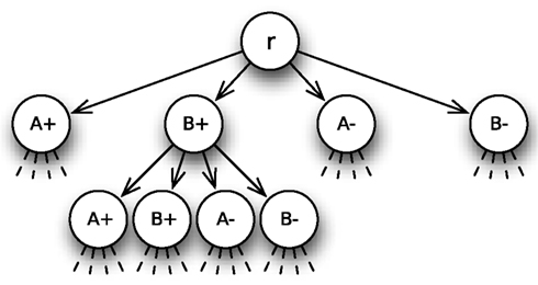
Figure 1. 4-ary tree for choice between two alternatives A and B. The root r has four outgoing edges directing to four vertices that represent the counters A⁺, A⁻, B⁺, and B⁻. Each of these vertices has four outgoing edges and thus four children itself, and so forth.

FIGURE 2

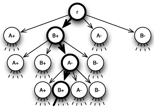
Figure 2. 4-ary tree for choice between two alternatives A and B with highlighted sample path r → B⁺ → A⁻ → B⁺ → ‥.

Three features of the model are of specific interest: (a) when and how the walk starts after presentation of choice alternatives (in an experimental trial), (b) how the walk chooses the next edge to pass through in each step, and (c) when and how the walk stops. Without an a priori bias toward any of the choice alternatives, we assume that all counter states are set to zero at the outset of the information sampling process and hence, the process starts with presentation of the choice alternatives. Biases toward one or several of the alternatives can be implemented by either defining initial values unequal to zero for these alternatives or by independently sampling information for the alternatives from predefined distributions for some time before the actual information sampling process starts (cf. Diederich and Busemeyer, 2006; Diederich, 2008). For simplicity, we assume no biases here, i.e., initial values are set to zero for all alternatives. Note that for the 2N-ary choice tree, initial values are counter states at the root r. Then the walk moves away from there step by step, choosing the next edge to pass through by means of so-called transition probabilities p_e, e ∈ E. The transition probabilities are built up of the comparison of the alternatives the decision maker considers and supplemented with a counter-dependent component and a random component. For each vertex, the transition probabilities for all outgoing edges sum up to one, so that the walk does not stay still at any vertex it reaches throughout the information sampling process. We show the structure of the model first; a detailed description of the transition probabilities is presented in the next section. For simplicity consider a choice situation with two alternatives A and B; the counter-dependent component and the random component are set to zero. As shown in Figure 3, transition probabilities are the same for the outgoing edges of each vertex v ∈ V, i.e., $p_{\left(v,v\left(A^{+}\right)\right)}=p\left(A^{+}\right)$ for each edge (v,v(A⁺)) ∈ E leading to a vertex with label A⁺, $p_{\left(v,v\left(B^{+}\right)\right)}=p\left(B^{+}\right)$ for each edge leading to a vertex with label B⁺ and so on for the other counters A⁻ and B⁻. The probability for walking along a specific path is the product of transition probabilities of all edges on that path. In our example, the probability p for making the first three steps as shown in Figure 2 is p = p(B⁺)·p(A⁻)·p(B⁺).

FIGURE 3

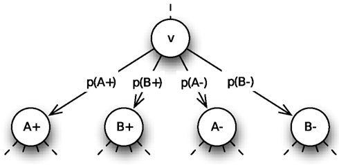
Figure 3. Transition probabilities for the two-alternative choice problem with no counter-dependent and random component. p(A⁺), p(B)⁺, p(A)⁺, and p(B⁻) sum up to one and are the same for the outgoing edges of each vertex v ∈ V.

The third topic addresses the stopping rule, that is, when the decision maker stops sampling information and chooses a choice alternative. A specific stopping rule depends on the preference states associated with the alternatives, i.e., the differences of their respective two counters which are compared to certain thresholds θ. The thresholds can be defined in several ways, their suitability depending on the definition of transition probabilities and initial values. They are (1) one single positive threshold θ⁺ > 0 for all alternatives, (2) one positive and one negative threshold θ⁺ > 0 and θ⁻ < 0 for all alternatives, (3) a positive threshold ${\theta }_i^{+}$ for each alternative i ∈ {1, …, N}, and (4) a positive and a negative threshold ${\theta }_i^{+}$ and ${\theta }_i^{-}$ for each alternative i ∈ {1, …, N}.

Obviously, the simplest setup is a single positive threshold θ⁺ > 0 for all alternatives, which is hit as soon as the information sampled in favor of any/one of the alternatives exceeds the information against it by θ⁺ for the first time, i.e., when Pref(i) = θ⁺ for one alternative i ∈ {1, …, N}. Sometimes, however, the probability for collecting negative information may be greater than the probability for sampling information in favor of these alternatives and reaching a positive threshold θ⁺ is very unlikely. For those situations it is useful to introduce a second, negative threshold, θ⁻ < 0, which is hit when negative information of one alternative exceeds the positive information of this alternative by −θ⁻, i.e., Pref(i) = θ⁻. In this case the respective alternative is not chosen but withdrawn from the choice set and the sampling process continues with one alternative less as described in the next paragraph. Note, that in both cases the thresholds are global in the sense that the same thresholds apply for all choice alternatives. Finally, θ⁺ (and θ⁻) may vary from alternative to alternative, yielding one (or two) thresholds ${\theta }_i^{+}$ (and ${\theta }_i^{-}$) for each of N alternatives, i ∈ {1, …, N}. Here the thresholds are local in the sense that each alternative has its own threshold(s). This is an alternative way to implement biases when the initial values are zero. That is, biases do not affect transition probabilities through the counter-dependent component and can thus be interpreted as the decision maker’s stable opinion about the presented alternatives.

Withdrawal of alternatives from a choice set traces back to the model of elimination by aspects (EBA model, Tversky, 1972). But whereas elimination is the only means to come to a decision in the EBA model, the 2N-ary choice tree model like the multi-alternative DFT (Roe et al., 2001) provides several ways to reach a decision. An alternative i is chosen either if its preference state exceeds ${\theta }_i^{+}$ or if all other alternatives have been withdrawn from the choice set or a combination of these two. Figure 4 shows three examples of walks that lead to the choice of alternative B from a set of three alternatives A, B, and C with global thresholds θ⁺ = 2 and θ⁻ = −2. The leftmost walk represents direct choice of alternative B, the rightmost withdrawal of alternative C and subsequent choice of option B and the middle walk illustrates withdrawal of alternative A first and then of option C. Note that after withdrawal of one alternative, there are two-outgoing edges less from the respective vertex downward. Transition probabilities change accordingly, i.e., the withdrawn alternative is removed from the comparison procedure and its counter states no longer contribute to the counter-dependent component (cf. next section). This corresponds to an anew started information sampling process between the remaining alternatives and their previous counter states as initial values.

FIGURE 4

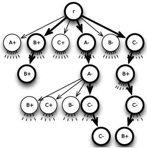
Figure 4. 6-Ary tree for choice between three alternatives A, B, and C with decision thresholds θ⁺ = 2 and θ⁻ = 2 and three-different sample paths that lead to choice of alternative B.

For a choice set with N alternatives and given thresholds ${\theta }_i^{\pm }$ this defines the structure of the 2N-ary choice tree. For each alternative i ∈ {1, 2, …, N} we can thus completely identify the set V_i ⊆ V of vertices where alternative i is chosen. Defining P_v: = P_{{r, v}} to be the unique path from the root r to a vertex v ∈ V and given transition probabilities p_e for all edges e ∈ E we can identify the probability for walking along a path P_v as the product $p_v={\Pi }_{e\in P_v}{p}_e$ and therewith define:

Definition 2 (expected choice probability): The expected probability for choosing alternative i ∈ {1, 2, …, N} is the probability for reaching the set V_i:

$p_i=\sum _{v\in V_i}\prod _{e\in P_v}{p}_e.$ (1)

The length |P_v| of the path P_v from r to v ∈ V indicates the number of steps that the random walk has to take to reach v. Multiplied by the length h of the time interval, this yields the time it takes to cover the distance from r to v. Thus T_v = h·|P_v|.

Definition 3 (expected hitting time): The expected time for choosing alternative i ∈ {1, 2, …, N} is the sum of expected hitting times for each vertex v ∈ V_i weighted by the probability for reaching v:

$\mathbb{E}\left[T_i\right]=h\cdot \sum _{v\in V_i}\left|P_v\right|\cdot p_v=h\cdot \sum _{v\in V_i}\left|P_v\right|\cdot \prod _{e\in P_v}{p}_e.$ (2)

The expected choice probabilities and hitting times can be approximated up to absolute accuracy in finite time. See below for the formal statement and proof of this property.

2.2. Transition Probabilities

Having defined the skeletal structure of our theory, we can now proceed to its heart, the transition probabilities. The main components are (a) weighted comparison of alternatives, (b) mutual or global inhibition, (c) decay of already sampled information over time, and (d) a random part. The transition probabilities control the information sampling process and thus describe the development of human preferences in specific choice situations. Throughout this section we will consider such situations with N choice alternatives that are evaluated with respect to the same D attributes. For each alternative, the decision maker is provided with one non-negative value per attribute, representing an objective evaluation of that alternative with respect to the attributes. The N·D values in total can be stored in a N × D-matrix L = (l_ij) with i = 1, …, N and j = 1, …, D.

The definition of transition probabilities is based on weighted integration of results of an attribute-wise comparison of alternatives. To ensure equally significant impact of the weight parameters, preprocessing of the values of the alternatives with respect to the attributes is necessary and we do so by separately normalizing them to one for each attribute. This yields a new matrix $M=\left(m_{ij}\right)=\left(l_{ij}∕{\sum }_{k=1}^N{l}_{kj}\right)$ with i = 1, …, N and j = 1, …, D and thus column sum ${\sum }_{i=1}^N{m}_{ij}=1$ for all j ∈ {1, …, D}.

2.2.1. Comparison of alternatives

At first we focus on one attribute j only. The easiest way to define transition probabilities is simply to use the entries from the respective column j of M and assign them to the edges that affiliate with the counters for positive information. The counters for negative information get transition probabilities zero. This corresponds to a framework where the alternatives are compared to an inferior external reference point (e.g., cars A, B, and C are compared to not having a car at all). Because the values for each attribute sum up to one already, no further normalization is needed.

We differentiate between external reference points that are not part of the choice set and internal reference points that are part of the choice set and available for the decision maker. For instance, if someone moves to a new city and has to choose between several available apartments, she will probably compare them to her old apartment which is no longer available in the new city and thus an example for an external reference point. Or consider a choice of dessert in a restaurant when the decision maker is told that the chocolate cake she ordered is no longer available because someone just had the last piece. An internal reference point, however, is part of the choice set, actually several or even all available alternatives can be used as internal reference points at the same time, possibly in combination with an external reference point.

Having decided which reference points to use, the alternatives i ∈ {1, …, N} are compared to them. For each alternative i, favorable and unfavorable comparisons are handled separately and the absolute values of their differences are summed up to obtain measures of evidence for and against alternative i, respectively. This yields two non-negative values per alternative and thus 2N values in total that are then normalized to one in order to obtain probabilities. In the car example where three cars are compared to not having a car at all, probabilities associated with negative counters are set to zero as each car is better than, presumably, no car. Actually, whenever one single reference point is used, at least half of the probabilities are zero because each alternative is either favored over the reference point or not and hence there cannot be evidence for and against one alternative at the same time. However, our main focus is on situations where each of at least three alternatives in the choice set is used as internal reference point for all the other alternatives and thus there are at least two-reference points.

In this case we obtain a vector

$P_j=\left(\begin{array}{c}\hfill p_{1j}\hfill \\ \hfill ⋮\hfill \\ \hfill p_{Nj}\hfill \\ \hfill p_{\left(N+1\right)j}\hfill \\ \hfill ⋮\hfill \\ \hfill p_{\left(2N\right)j}\hfill \\ \hfill \hfill \end{array}\right)=\left(\begin{array}{c}\hfill p_{1j}^{+}\hfill \\ \hfill ⋮\hfill \\ \hfill p_{Nj}^{+}\hfill \\ \hfill p_{1j}^{-}\hfill \\ \hfill ⋮\hfill \\ \hfill p_{Nj}^{-}\hfill \\ \hfill \hfill \end{array}\right)∕\sum _{i=1}^N\left(p_{ij}^{+}+p_{ij}^{-}\right)$

with

$\begin{array}{rcll}{p}_{ij}^{+}& =\sum _{k\ne i}\left(m_{ij}-m_{kj}\right)\cdot I\left(m_{ij}>m_{kj}\right),& & \\ p_{ij}^{-}& =\sum _{k\ne i}\left(m_{kj}-m_{ij}\right)\cdot I\left(m_{ij}<m_{kj}\right)& & \end{array}$

for k = 1, …N and

$\mathbb{I}\left(x\right)=\left\{\begin{array}{cc}1,\hfill & \text{if}x\text{is}\text{true}\hfill \\ 0,\hfill & \text{else}.\hfill \\ \hfill \end{array}\right.$

Especially with an external reference point at hand, the actual choice may lead to a loss of some kind. For instance, in the apartment example above a loss could be a further way to the workplace or a smaller bathroom. People usually try to avoid losses more than they seek gains while overrating small losses and gains compared to larger ones (Kahneman and Tversky, 1991; Tversky and Simonson, 1993). The 2N-ary choice tree model can account for the loss-aversion principle (Kahneman and Tversky, 1979) with an asymmetric value function (Kahneman and Tversky, 1979; Tversky and Simonson, 1993) by increasing probabilities for sampling negative information compared to probabilities for gathering positive information.

In their LCA model, Usher and McClelland (2004) use an asymmetric value function

$V\left(x\right)=\left\{\begin{array}{cc}log\left(1+x\right),\hfill & \text{for}x>0\hfill \\ -\left[log\left(1+\left|x\right|\right)+log{\left(1+\left|x\right|\right)}^2\right],\hfill & \text{for}x<0\hfill \end{array}\right.$

and apply it to the relative advantages (x > 0) and disadvantages (x < 0) of alternatives compared to each other on one dimension. V(x) is steeper for losses than for gains but flattens for both advantages and disadvantages when they become bigger. This favors similar pairs of alternatives over dissimilar ones and allows the LCA model to account for attraction and compromise effects.

Adopting it to our 2N-ary choice tree model this yields an asymmetric value function

$A\left(x\right)=\left\{\begin{array}{cc}log\left(1+x\right),\hfill & \text{for}\text{favorable}\text{comparisons}\hfill \\ log\left(1+x\right)\hfill \\ +log{\left(1+x\right)}^2,\hfill & \text{for}\text{unfavorable}\text{comparisons,}\hfill \\ \hfill \end{array}\right.$

which can be applied to the absolute differences from the comparison process before normalizing them to one:

$\begin{array}{llll}{p}_{ij}^{+}& =\sum _{k\ne i}A\left(m_{ij}-m_{kj}\right)\cdot \mathbb{I}\left(m_{ij}>m_{kj}\right),& & \\ p_{ij}^{-}& =\sum _{k\ne i}A\left(m_{kj}-m_{ij}\right)\cdot \mathbb{I}\left(m_{ij}<m_{kj}\right).& & \end{array}$

The asymmetric value function A(x) is not necessary for explanation of similarity, attraction, or compromise effects in the 2N-ary choice tree model but moderates the strength of the compromise effect (see below). In cases where θ⁺ and θ⁻ have the same order of magnitude, application of A(x) leads to faster withdrawal of alternatives and hence, more decisions are based on withdrawal of all but one alternative.

In summary, the comparison of alternatives provides us with a set of 2N transition probabilities for each attribute j ∈ {1, …, D} that form a vector P_j. Each of these vectors can be used to model an information sampling process based on a single attribute. As the probabilities are derived from comparison of alternatives only, they remain constant during the whole process.

2.2.2. Weighting of attributes

So far we have only focused on one attribute but choice alternatives in real life are most often described by several attributes and thus require more elaboration. In the following, we consider choice sets with N alternatives characterized by D ≥ 2 attributes. Especially situations with three alternatives where similarity, attraction or compromise effects have been observed, require at least two attributes to distinguish the different alternatives from each other. Note that it is difficult to construct a choice set with two equally attractive but different alternatives due to the decision maker’s individual salience. Diederich (1997) accounts for subjective salience by defining a Markov process on the attributes giving probabilities for switching attention from one attribute to the other. This process can be directly implemented into the transition probabilities by using a stationary distribution on the attributes. Each attribute j ∈ {1, …, D} is assigned a weight w_j that corresponds to the probability for considering this attribute during the information sampling process. For each alternative i ∈ {1, …, N} weighted positive and negative evidence is added up and normalized to obtain a proper probability distribution (the probabilities add up to one), that is

$P=\left(\begin{array}{c}\hfill p_1\hfill \\ \hfill ⋮\hfill \\ \hfill p_N\hfill \\ \hfill p_{\left(N+1\right)}\hfill \\ \hfill ⋮\hfill \\ \hfill p_{\left(2N\right)}\hfill \\ \hfill \hfill \end{array}\right)=\left(\begin{array}{c}\hfill p_1^{+}\hfill \\ \hfill ⋮\hfill \\ \hfill p_N^{+}\hfill \\ \hfill p_1^{-}\hfill \\ \hfill ⋮\hfill \\ \hfill p_N^{-}\hfill \\ \hfill \hfill \end{array}\right)∕\sum _{i=1}^N\left(p_i^{+}+p_i^{-}\right)$

with $p_i^{+}={\sum }_{j=1}^D\left(p_{ij}^{+}\cdot w_j\right)$ and $p_i^{-}={\sum }_{j=1}^D\left(p_{ij}^{-}\cdot w_j\right)$ for i ∈ {1, …, N}.

The weights account for subjective salience that in turn may be influenced by several internal and external factors such as personal preferences, social influences, characteristics of the choice set, or the experimenter’s instructions. Personal preferences like, for instance, the preference of time over money or of tastiness to healthiness may be learned from friends, family, or other people in our surrounding. They are generally independent from the choice situation and hence, their impact on the information sampling is indirect. On the contrary, the choice set itself has a direct influence on the subjective saliences. For example, the decision maker may primarily focus on those attributes where alternatives are very similar to each other, because this information may be crucial for the choice. Or she concentrates on attributes with somehow outstanding values. It is therefore important to normalize the values for each attribute as described before because this guarantees representation of these effects by the attention weights. People that are present during the deliberation process like sales people or immediately prior to it like the experimenter in a laboratory context can also have a direct influence on the saliences by drawing the decision maker’s attention to a specific attribute. This can be used to verify influence of attention weights by instructing decision makers to focus on certain attributes while choosing between different cars, salad dressings, chocolate bars or shoes. Corresponding experiments are under way.

2.2.3. Noise

In order to account for random fluctuations in the decision maker’s attention (cf. Busemeyer and Townsend, 1993) which are independent of the characteristics of the choice alternatives, we add a constant to each transition probability. This makes every outgoing edge of a vertex v ∈ V available for the next (random) step because it guarantees non-zero transition probabilities for all of them. Let 𝒩 be a vector of length 2N with all entries equal to 1/2N. Weighting the transition probabilities P from the weighted comparison of alternatives by (1 − ξ) with 0 ≤ ξ ≤ 1 and adding the product ξ · 𝒩 yields noisy transition probabilities where ξ moderates the strength of the uniformly distributed noise:

$P_{𝒩}=\left(1-\xi \right)\cdot P+\xi \cdot 𝒩.$

The vector P_𝒩 of noisy transition probabilities integrates comparison of alternatives on all present attributes. Related to the 2N-ary choice tree, this information is global as it is independent of the local counter states and thus the transition probabilities are the same for the edges emanating from each vertex.

2.2.4. Leakage

During their development of DFT (Busemeyer and Townsend, 1993) introduce a factor s for serial positioning effects, called “growth-decay rate.” It produces recency effects for 0 < s < 1 and primacy effects for s < 0. In their multi-alternative version of DFT (Roe et al., 2001) the reverse (1 − s) of this factor reappears as “self-feedback loop” and accounts for the memory of previous preference states. (1 − s) = 1 denotes perfect memory of the previous state (1 − s) = 0 no memory at all. For their simulations (Roe et al., 2001) use (1 − s) = 0.94 or (1 − s) = 0.95. Usher and McClelland(2001, 2004) adopted the idea of the self-feedback loop, but call it “leakage” λ and – based on findings from neuroscience – interpret it as “neural decay.”

In order to account for decay of already sampled information over time, we implement leakage ℒ into our transition probabilities. Leakage obviously depends on already sampled information and thus we normalize the current states of our 2N counters to 1 − λ and for each alternative i ∈ {1, …, N} add the result for the positive (negative) counter of alternative i to the transition probability associated with the negative (positive) counter for alternative i weighted by λ. Like this, the overall sum of the transition probabilities remains 1 and only 100·λ% of the sampled information is actually memorized. The greater λ, the longer it takes until the process reaches a threshold. Overall, this yields

$P_{𝒩ℒ}=\left(1-\lambda \right)\cdot \left[\left(1-\xi \right)\cdot P+\xi \cdot 𝒩\right]+\lambda \cdot ℒ.$

2.2.5. Inhibition

To account for the similarity, attraction, and compromise effect, DFT (Roe et al., 2001) and the LCA model (Usher and McClelland, 2004) both rely on inhibition. Whereas distance-dependent inhibition enables DFT to account for the attraction and compromise effect, global inhibition produces the similarity effect in the LCA model. We can implement both types of inhibition into the 2N-ary choice tree model to explore their impact on the aforementioned effects. We define weights for all pairs of alternatives by either using the same weight for all pairs like Usher and McClelland (2004) do with their “global inhibition” parameter β or different weights like Roe et al. (2001) do with their distance-dependent weights (i.e., higher weights for more similar alternatives). Those weights can be stored in a symmetric N × N-matrix with zeros on the diagonal.

Taking into account the basic concept of inhibition, we assume that the state of the positive counter for each alternative i ∈ {1, …, N} reduces sampling of positive information for all other alternatives j ∈ {1, …, N} − {i}. Because this is equivalent to increasing sampling of negative information for these alternatives and vice versa for states of negative counters, we implement inhibition ℐ into our model as follows: Multiplying the symmetric N × N-matrix with both the vector of states of positive counters and negative counters yields two vectors with weighted sums of counter states. We concatenate them in inverted order and normalize the resulting vector of length 2N to μ before adding it to the vector of transition probabilities now weighted by (1 − λ − μ). This completes the final definition of transition probabilities

$P_{𝒩ℒℐ}=\left(1-\lambda -\mu \right)\cdot \left[\left(1-\xi \right)\cdot P+\xi \cdot 𝒩\right]+\lambda \cdot ℒ+\mu \cdot ℐ.$

In a nutshell, the transition probabilities consist of a global part that is independent from the current counter states of the random walk and a local part that depends on already sampled information. The global parts are weighted sums of comparative values P and noise 𝒩 that remain constant during the whole process. They are complemented with leakage ℒ and inhibition ℐ which may change from step to step and hence, are local in the terminology of the 2N-ary choice tree model.

3. Predictions of the 2N-ary Choice Tree Model

To show the predictions of the 2N-ary choice tree model and how it accounts for similarity, attraction, and compromise effects in choice settings with three alternatives characterized by two attributes, we run several simulations. An extension to more alternatives is straightforward. We will define values l_ij that range between 0 and 10. As values of choice alternatives are normalized to one on each dimension before comparison, only the relative amount of these values is of importance. Unless stated otherwise, we run 1000 trials per simulation with threshold θ = 20, noise factor ξ = 0.01 and leakage factor λ = 0.05, but without inhibition (i.e., μ = 0).

In order to meet the assumptions of the similarity, attraction, and compromise effect, we constructed two equally attractive but dissimilar alternatives A = (9, 1) and B = (1, 9) that are both evaluated with respect to two attributes. The choice probabilities were 0.52, 0.51, and 0.47 for alternative A and 0.48, 0.49, and 0.53 for option B in three simulations with the above mentioned parameters and attribute weight 0.5 for both attributes.

To reproduce the similarity effect (Simonson, 1989) we add a third alternative to the choice set that is equal or similar to either option A or B, i.e., C = (1, 9), C₂ = (0.9, 9.1), or C₃ = (1.1, 8.9). To prevent a combination of the similarity effect with a slight compromise effect (cf. Usher and McClelland, 2004), we will use only C for demonstration, but the results for options C₂ and C₃ are very similar to the ones presented here. The alternatives are put together in a 3 × 2-matrix L, whose columns are normalized to one, resulting in matrix M:

$L=\left(\begin{array}{cc}\hfill 9\hfill & \hfill 1\hfill \\ \hfill 1\hfill & \hfill 9\hfill \\ \hfill 1\hfill & \hfill 9\hfill \\ \hfill \hfill \end{array}\right)\text{and}M=\left(\begin{array}{cc}\hfill 0.818\hfill & \hfill 0.053\hfill \\ \hfill 0.091\hfill & \hfill 0.474\hfill \\ \hfill 0.091\hfill & \hfill 0.474\hfill \\ \hfill \hfill \end{array}\right).$

M already shows smaller values for alternatives B and C on the second dimension than for alternative A on dimension one which characterizes the similarity effect. In the next step, the values on each dimension are compared to each other, resulting in a 6 × 2-matrix that is then multiplied by $W=\left(\begin{array}{c}\hfill 0.4\hfill \\ \hfill 0.6\hfill \\ \hfill \hfill \end{array}\right)$ before being normalized to one again:

$P^{\prime }=\left(\begin{array}{cc}\hfill 1.4545\hfill & \hfill 0\hfill \\ \hfill 0\hfill & \hfill 0.4211\hfill \\ \hfill 0\hfill & \hfill 0.4211\hfill \\ \hfill 0\hfill & \hfill 0.8421\hfill \\ \hfill 0.7273\hfill & \hfill 0\hfill \\ \hfill 0.7273\hfill & \hfill 0\hfill \\ \hfill \hfill \end{array}\right)\cdot \left(\begin{array}{c}\hfill 0.4\hfill \\ \hfill 0.6\hfill \\ \hfill \hfill \end{array}\right)=\left(\begin{array}{c}\hfill 0.5818\hfill \\ \hfill 0.2526\hfill \\ \hfill 0.2526\hfill \\ \hfill 0.5053\hfill \\ \hfill 0.2909\hfill \\ \hfill 0.2909\hfill \\ \hfill \hfill \end{array}\right).$

and

$P=\left(\begin{array}{c}\hfill 0.5818\hfill \\ \hfill 0.2526\hfill \\ \hfill 0.2526\hfill \\ \hfill 0.5053\hfill \\ \hfill 0.2909\hfill \\ \hfill 0.2909\hfill \\ \hfill \hfill \end{array}\right)∕2.1742=\left(\begin{array}{c}\hfill 0.2676\hfill \\ \hfill 0.1162\hfill \\ \hfill 0.1162\hfill \\ \hfill 0.2324\hfill \\ \hfill 0.1338\hfill \\ \hfill 0.1338\hfill \\ \hfill \hfill \end{array}\right)$

Finally noise is added to this constant part of the transition probabilities. In contrast to leakage that depends on the respective counter states and has to be computed anew for every step, P_𝒩 remains constant over time. The only occasion where it changes is after withdrawal of one alternative from the choice set.

The most interesting parameters in this attempt to model a similarity effect are the attribute weights as they control the strength of the effect. Figure 5 demonstrates this by means of choice probabilities from simulations with different sets of attribute weights but otherwise unchanged parameters. It starts with $W=\left(\begin{array}{c}\hfill 0.6\hfill \\ \hfill 0.4\hfill \\ \hfill \hfill \end{array}\right)$ and $W=\left(\begin{array}{c}\hfill 0.55\hfill \\ \hfill 0.45\hfill \\ \hfill \hfill \end{array}\right)$ on the left side and gradually changes by 0.05 to $W=\left(\begin{array}{c}\hfill 0.25\hfill \\ \hfill 0.75\hfill \\ \hfill \hfill \end{array}\right)$ on the right side. The relative frequency of choices for alternatives A, B, and C including the mean number of steps leading to these choices can be found in Table 1.

FIGURE 5

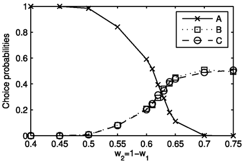
Figure 5. Choice probabilities for choice between three alternatives A = (9, 1), B = (1, 9), and C = (1, 9) and different attention weights w₁ and w₂ for the two attributes. The abscissa is labeled with increasing values of w₂ corresponding to decreasing values of w₁. For w₂ < 0.625 a similarity effect can be observed.

TABLE 1

Table 1. Relative number of choices and mean response times (arbitrary unit, in parentheses) for alternatives A = (9, 1), B = (1, 9), and C = (1, 9) from 1000 simulations with θ = 20, ξ = 0.01, λ = 0.05, μ = 0, and w₂ = 1 − w₁ ranging from 0.4 to 0.75 as indicated in the first row.

The same mechanisms account for the attraction effect (Huber et al., 1982) that occurs during choice between two equally attractive but dissimilar alternatives A and B and a third alternative C that is similar to one of these but slightly less attractive. For A = (9, 1), B = (1, 9), and C = (1, 8.5) this yields

$L=\left(\begin{array}{cc}\hfill 9\hfill & \hfill 1\hfill \\ \hfill 1\hfill & \hfill 9\hfill \\ \hfill 1\hfill & \hfill 8.5\hfill \\ \hfill \hfill \end{array}\right)\text{and}M=\left(\begin{array}{cc}\hfill 0.818\hfill & \hfill 0.054\hfill \\ \hfill 0.091\hfill & \hfill 0.487\hfill \\ \hfill 0.091\hfill & \hfill 0.459\hfill \\ \hfill \hfill \end{array}\right).$

As shown in Figure 6, the attraction effect occurs between $W=\left(\begin{array}{c}\hfill 0.39\hfill \\ \hfill 0.61\hfill \\ \hfill \hfill \end{array}\right)$ and $W=\left(\begin{array}{c}\hfill 0.35\hfill \\ \hfill 0.65\hfill \\ \hfill \hfill \end{array}\right)$ Note that the deviation from weights w₁ = w₂ = 0.5 is due to a higher salience of attribute two because the values on this attribute differentiate between the alternatives. The relative frequency of choices for alternatives A, B, and C including the mean number of steps leading to these choices can be found in Table 2.

FIGURE 6

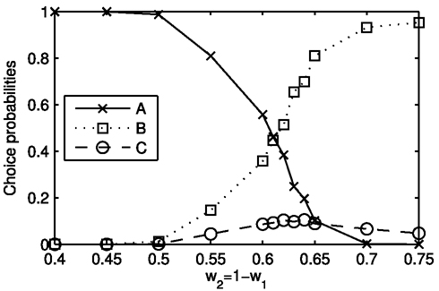
Figure 6. Choice probabilities for choice between three alternatives A = (9, 1), B = (1, 9), and C = (1, 8.5) and different attention weights w₁ and w₂ for the two attributes. The abscissa is labeled with increasing values of w₂ corresponding to decreasing values of w₁. For 0.61 ≤ w₂ < 0.65 an attraction effect can be observed.

TABLE 2

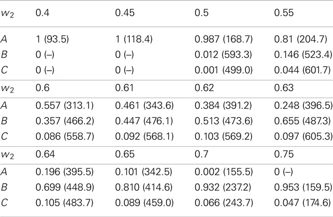
Table 2. Relative number of choices and mean response times (arbitrary unit, in parentheses) for alternatives A = (9, 1), B = (1, 9), and C = (1, 8.5) from 1000 simulations with θ = 20, ξ = 0.01, λ = 0.05, μ = 0, and w₂ = 1 − w₁ ranging from 0.4 to 0.75 as indicated in the first row.

For the compromise effect (Simonson, 1989), two equally attractive but dissimilar alternatives A = (9, 1) and B = (1, 9) compete against a compromise option C = (5, 5). Note that the defined values for each alternative sum up to ten and thus all three alternatives objectively are equally attractive provided the attributes are equally weighted. We get

$L=\left(\begin{array}{cc}\hfill 9\hfill & \hfill 1\hfill \\ \hfill 1\hfill & \hfill 9\hfill \\ \hfill 5\hfill & \hfill 5\hfill \\ \hfill \hfill \end{array}\right)\text{and}M=\left(\begin{array}{cc}\hfill 0.6\hfill & \hfill 0.067\hfill \\ \hfill 0.067\hfill & \hfill 0.6\hfill \\ \hfill 0.333\hfill & \hfill 0.333\hfill \\ \hfill \hfill \end{array}\right),$

and restricting w₁ = w₂ = 0.5 to be equal, this yields

$P=\left(\begin{array}{c}\hfill 0.4\hfill \\ \hfill 0.4\hfill \\ \hfill 0.2667\hfill \\ \hfill 0.4\hfill \\ \hfill 0.4\hfill \\ \hfill 0.2667\hfill \\ \hfill \hfill \end{array}\right).$

So far, these transition probabilities do not seem to induce any compromise effect but as the probabilities for sampling negative information are comparatively high, withdrawal of one alternative from the choice set frequently occurs in that setting. After withdrawal of one alternative, comparison of the remaining alternatives is renewed. In the cases where alternative A or B are withdrawn, the new probabilities clearly favor the compromise option C, yielding an overall preference for that alternative:

$M_{-A/-B}=\left(\begin{array}{cc}0.643& 0.167\\ 0.357& 0.833\end{array}\right),P_{-A/-B}=\left(\begin{array}{c}0.15\\ 0.35\\ 0.35\\ 0.15\end{array}\right).$

In 1000 trials with decision threshold θ = 20, noise factor ξ = 0.01, leakage factor λ = 0.05, and no inhibition, alternatives A and B were chosen 247 (24.7%) and 250 (25%) times, respectively, and option C won 503 (50.3%) decisions. Decreasing θ to 10 yields choice frequencies of 243 (24.3%) for alternative A, 267 (26.7%) for option B, and 490 (49%) for alternative C. θ = 5 leads to 253 (36.9%) choices with an average step number of 36.9 for alternative A, 269 (26.9%) choices with 38.3 steps on average for option B, and 478 (47.8%) choices with 43.8 steps on average for alternative C. Figure 7 shows the response time distribution for alternative A for θ = 5, ξ = 0.01, λ = 0.05, and μ = 0. The expected response time, i.e., the mean of the distribution is 36.6. The magnitude of the compromise effect can be influenced by application of an asymmetric value function after comparison of alternatives.

FIGURE 7

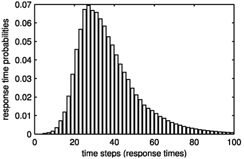
Figure 7. Response time distribution for alternative A = (9, 1) in the compromise setup with θ = 5, ξ = 0.01, λ = 0.05, and μ = 0. The expected response time, i.e., the mean of the distribution is 36.6.

4. Comparison with Other Models

Multi-alternative DFT (Roe et al., 2001) and the LCA model (Usher and McClelland, 2004) both account for similarity, attraction, and compromise effects in three-alternative preferential choice and thus build the theoretical background for the 2N-ary choice tree model. Nevertheless there are some important differences and the first one to set the new model apart from the previous approaches is the attribute-wise normalization of the initially provided evaluations of alternatives. This preprocessing of input values makes them comparable over attributes. Effects that originate from differing orders of magnitude of the input values can thus be controlled by influencing the attention weights for the attributes. The comparison of alternatives on single attributes is basically the same in all three models but only the LCA model and the 2N-ary choice tree model allow for external reference points that are not present in the choice set to influence the resulting values. Application of an asymmetric value function allows the LCA model to implement the loss-aversion principle (Kahneman and Tversky, 1979) and addition of a positive constant avoids negative activations and thus negated inhibition which was crucial for some of the results of multi-alternative DFT. Both concepts (asymmetric value function and positive constant) can be implemented into the 2N-ary choice tree model as well but do not affect its ability to account for the aforementioned effects (except for the magnitude of the compromise effect). Whereas all three models use leakage to account for decay of already sampled information over time and have a random part that implements noise in human decision making, inhibition is another crucial difference between them. In multi-alternative DFT, local inhibition explains the attraction and compromise effect, the LCA model uses global inhibition to account for the similarity effect. Both types of inhibition can be implemented in the 2N-ary choice tree model but are not necessary for explanation of the three effects.

Beside some similarities and dissimilarities between the models, in particular with respect to some underlying psychological concepts the 2N-ary choice tree model is the first to provide expected choice probabilities and response times in closed form and thus allows for convenient estimation of the model parameters from the observed choice times and frequencies in experimental settings. Furthermore, it can be extended to more than three-choice alternatives in a straightforward way to account for choice behavior in more complex, and possibly more realistic choice situations.

5. Concluding Remarks

The 2N-ary choice tree model provides alternative explanations for the similarity, attraction, and compromise effect that can be experimentally tested as suggested before. Especially the manipulation of attention weights is of interest, because it differentiates the model on hand from former approaches and should allow to experimentally produce similarity and attraction effects which has been proven to be difficult in the past. One problem, however, we are currently encountering is limited machine accuracy which leads to accumulation of rounding errors during calculation of expected choice probabilities and response times.

6. Formal Statement and Proof

We can approximate the expected choice probabilities and hitting times up to absolute accuracy in finite time. This follows from Theorem 1:

Theorem 1: Each random walk Y_n on the above defined tree T = (V, E, r) with transition probabilities p_e, ends in finite time with probability one.

Corollary 1: With probability one only finitely many addends in equations (1) and (2) are unequal zero.

Considering expected values, i.e., limits of infinite sums, it is helpful to make use of a concept that allows for propositions about asymptotic behavior. For each alternative, the difference of the two counters that are associated with this alternative resemble a birth-death chain:

Definition 4 (birth-death chain): A sequence of random variables X₁, X₂, … with values in a countable state space 𝒮 ≡ {0, 1, 2, …} ⊆ 𝒩 is called Markov chain, if it satisfies the Markov property

$\begin{array}{llll}& \mathbb{P}\left[X_{n+1}=x|X_1=x_1,X_2=x_2,\dots ,X_n=x_n\right]& & \\ & =\mathbb{P}\left[X_{n+1}=x|X_n=x_n\right].& & \end{array}$

A Markov chain is called time homogeneous, if ℙ[X_{n + 1} = x | X_n = y] = p(x, y) for all n, i.e., the probability for going from x to y is independent from n. A birth-death chain is a time homogeneous Markov chain that does not skip any state. Its transition probabilities p(x, y) are equal to zero for all x, y ∈ 𝒮 with |y − x| > 1. A non-homogeneous birth-death chain is a birth-death chain that is not time homogeneous.

Durrett (2010) proves the following theorem for (non-homogeneous) birth-death chains as special case of Markov chains:

Theorem 2: Let X_n be a Markov chain and suppose

$\mathbb{P}\left[{\cup }_{m=n+1}^{\infty }\left\{X_m\in B_m\right\}|X_n\right]\ge \delta >0\text{on}\left\{X_n\in A_n\right\}.$

Then ℙ[{X_n ∈ A_n infinitely often} − {X_n ∈ B_n infinitely often}] = 0.

For each alternative i ∈ {1, 2, …, N}, the above mentioned difference of its two counters can be interpreted as non-homogeneous birth-death chain X_n with absorbing states ${\theta }_i^{-}$ and ${\theta }_i^{+}$ and state space $𝒮=\left\{{\theta }_i^{-},\left({\theta }_i^{-}+1\right),\left({\theta }_i^{-}+2\right),\dots ,\left({\theta }_i^{+}-2\right),\left({\theta }_i^{+}-1\right),{\theta }_i^{+}\right\}.$ Its transition probabilities are

$\begin{array}{cc}{p}^n\left(x,x+1\right)& =p_x^n=p_i^n\left(x\right),\\ p^n\left(x,x-1\right)& =q_x^n=p_{N+i}^n\left(x\right),\\ p^n\left(x,x\right)& =r_x^n=1-p_x^n-q_x^n,\end{array}\}\text{\hspace{1em}\hspace{1em}for\hspace{0.17em}}x\in 𝒮-\left\{{\theta }_i^{-},{\theta }_i^{+}\right\}$

and

$\begin{array}{cc}{p}_x^n=q_x^n& =0\\ r_x^n& =1\end{array}\}\text{\hspace{1em}\hspace{1em}for\hspace{0.17em}}x\in \left\{{\theta }_i^{-},{\theta }_i^{+}\right\}.$

Due to the noise in the transition probabilities, $p_x^n>0$ and $q_x^n>0$ for all $x\in 𝒮-\left\{{\theta }_i^{-},{\theta }_i^{+}\right\}$ It follows that the probability for walking the direct way from $x\in 𝒮-\left\{{\theta }_i^{-},{\theta }_i^{+}\right\}$ to either ${\theta }_i^{-}$ or ${\theta }_i^{+}$ is

${\delta }_x:=\left(\prod _{y={\theta }_i^{-}+1}^x{q}_i^{n+x-y}\left(y\right)+\prod _{z=x}^{{\theta }_i^{+}-1}{p}_i^{n+z-x}\left(z\right)\right)>0$

and thus

$\delta :=\underset{{\theta }_i^{-}<x<{\theta }_i^{+}}{\min }{\delta }_x>0.$

Define $T_{{\theta }_i^{-}}=\inf \left\{n:X_n={\theta }_i^{-}\right\},T_{{\theta }_i^{+}}=\inf \left\{n:X_n={\theta }_i^{+}\right\},T_{{\theta }_i^{-}}\wedge T_{{\theta }_i^{+}},$ A_n = 𝒮, and $B_n=\left\{{\theta }_i^{-},{\theta }_i^{+}\right\}.$ Then {X_m ∈ B_m} is equivalent to T_i ≤ m and

$\mathbb{P}\left[{\cup }_{m=n+1}^{\infty }\left\{X_m\in B_m\right\}|X_n\right]=1>\delta$

for X_n ∈ B_n. The probability for walking from any x ∈ 𝒮 to either ${\theta }_i^{-}$ or ${\theta }_i^{+}$ on every possible way is

$\mathbb{P}\left[{\cup }_{m=n+1}^{\infty }\left\{X_m\in B_m\right\}|X_n\right]\ge \delta >0$

and thus fulfills the assumptions of Theorem 2. It follows that

$\mathbb{P}\left[\left\{X_n\in A_n\text{infinitely}\text{often}\right\}-\left\{X_n\in B_n\text{infinitely}\text{often}\right\}\right]=0$

which is equivalent to

$\mathbb{P}\left[\left\{X_n\in A_n-B_n\text{finitely}\text{often}\right\}\right]=\mathbb{P}\left[T_i<\infty \right]=1$

and as this is true for every alternative i ∈ {1, 2, …, N}, ℙ[T, ∞] = 1 holds for T:=minT₁, T₂, …, T_N. This proves Theorem 1.

Conflict of Interest Statement

The authors declare that the research was conducted in the absence of any commercial or financial relationships that could be construed as a potential conflict of interest.

Footnote

1. ^Definitions of graph-related terms not defined here can be found in Korte and Vygen (2002).

References

Busemeyer, J. R., and Townsend, J. T. (1992). Fundamental derivations from decision field theory. Math. Soc. Sci. 23, 255–282.

CrossRef Full Text

Busemeyer, J. R., and Townsend, J. T. (1993). Decision field theory: a dynamic-cognitive approach to decision making in an uncertain environment. Psychol. Rev. 100, 432–455.

Pubmed Abstract | Pubmed Full Text | CrossRef Full Text

Diederich, A. (1995). Intersensory facilitation of reaction time: evaluation of counter and diffusion coactivation models. J. Math. Psychol. 39, 197–215.

CrossRef Full Text

Diederich, A. (1997). Dynamic stochastic models for decision making under time constraints. J. Math. Psychol. 41, 260–274.

Pubmed Abstract | Pubmed Full Text | CrossRef Full Text

Diederich, A. (2008). A further test of sequential-sampling models that account for payoff effects on response bias in perceptual decision tasks. Percept. Psychophys. 70, 229–256.

Pubmed Abstract | Pubmed Full Text | CrossRef Full Text

Diederich, A., and Busemeyer, J. R. (2006). Modeling the effects of payoff on response bias in a perceptual discrimination task: bound-change, drift-rate-change, or two-stage-processing hypothesis. Percept. Psychophys. 68, 194–207.

Pubmed Abstract | Pubmed Full Text | CrossRef Full Text

Durrett, R. (2010). Probability: Theory and Examples, 4th Edn. New York: Cambridge University Press.

Hick, W. E. (1952). On the rate of gain of information. Q. J. Exp. Psychol. 4, 11–26.

CrossRef Full Text

Huber, J., Payne, J. W., and Puto, C. (1982). Adding asymmetrically dominated alternatives: violations of regularity and the similarity hypothesis. J. Consum. Res. 9, 90–98.

CrossRef Full Text

Hyman, R. (1953). Stimulus information as a determinant of reaction time. J. Exp. Psychol. 45, 188–196.

Pubmed Abstract | Pubmed Full Text | CrossRef Full Text

Kahneman, D., and Tversky, A. (1979). Prospect theory: an analysis of decision under risk. Econometrica 47, 263–291.

CrossRef Full Text

Kahneman, D., and Tversky, A. (1991). Loss aversion in riskless choice: a reference-dependent model. Q. J. Econ. 106, 1039–1061.

CrossRef Full Text

Koehler, D. J., and Harvey, N. (2007). Blackwell Handbook of Judgment and Decision Making, 2nd Edn. Oxford: Blackwell Publishing.

Korte, B., and Vygen, J. (2002). Combinatorial Optimization: Theory and Algorithms, 2nd Edn. Berlin: Springer.

LaBerge, D. (1962). A recruitment theory of simple behavior. Psychometrika 27, 375–396.

CrossRef Full Text

LaBerge, D. (1994). Quantitative models of attention and response processes in shape identification tasks. J. Math. Psychol. 38, 198–243.

CrossRef Full Text

Laming, D. R. J. (1968). Information Theory of Choice Reaction Times. New York: Academic Press.

Link, S. W., and Heath, R. A. (1975). A sequential theory of psychological discrimination. Psychometrika 40, 77–105.

CrossRef Full Text

Luce, D. (1986). Response Times. New York: Oxford University Press.

Pike, A. R. (1966). Stochastic models of choice behaviour: response probabilities and latencies of finite Markov chain systems. Br. J. Math. Stat. Psychol. 19, 15–32.

Pubmed Abstract | Pubmed Full Text | CrossRef Full Text

Ratcliff, R., and Smith, P. L. (2004). A comparison of sequential sampling models for two-choice reaction time. Psychol. Rev. 111, 333–367.

Pubmed Abstract | Pubmed Full Text | CrossRef Full Text

Roe, R. M., Busemeyer, J. R., and Townsend, J. T. (2001). Multialternative decision field theory: a dynamic connectionist model of decision making. Psychol. Rev. 108, 370–392.

Pubmed Abstract | Pubmed Full Text | CrossRef Full Text

Simonson, I. (1989). Choice based on reasons: the case of attraction and compromise effects. J. Consumer Res. 16, 158–174.

CrossRef Full Text

Smith, P. L., and Van Zandt, T. (2000). Time-dependent Poisson counter models of response latency in simple judgment. Br. J. Math. Stat. Psychol. 53, 293–315.

Pubmed Abstract | Pubmed Full Text | CrossRef Full Text

Townsend, J. T., and Ashby, F. G. (1983). The Stochastic Modeling of Elementary Psychological Processes. London: Cambridge University Press.

Tversky, A. (1972). Choice by elimination. J. Math. Psychol. 9, 341–367.

CrossRef Full Text

Tversky, A., and Simonson, I. (1993). Context-dependent preferences. Manage. Sci. 39, 1179–1189.

CrossRef Full Text

Usher, M., and McClelland, J. L. (2001). On the time course of perceptual choice: the leaky competing accumulator model. Psychol. Rev. 108, 550–592.

Pubmed Abstract | Pubmed Full Text | CrossRef Full Text

Usher, M., and McClelland, J. L. (2004). Loss aversion and inhibition in dynamical models of multialternative choice. Psychol. Rev. 111, 757–769.

Pubmed Abstract | Pubmed Full Text | CrossRef Full Text

Van Zandt, T., Colonius, H., and Proctor, R. W. (2000). A comparison of two response time models applied to perceptual matching. Psychon. Bull. Rev. 7, 208–256.

Pubmed Abstract | Pubmed Full Text | CrossRef Full Text