Corrigendum: ExGUtils: A Python Package for Statistical Analysis With the ex-Gaussian Probability Density
 Carmen Moret-Tatay
 Daniel Gamermann
 Esperanza Navarro-Pardo
 Pedro Fernández de Córdoba Castellá4
- 1Department of Neuropsychology, Methodology, Basic and Social Psychology, Faculty of Psychology, Universidad Católica de Valencia San Vicente Mártir, Valencia, Spain
- 2Instituto de Física, Universidade Federal do Rio Grande do Sul (UFRGS), Porto Alegre, Brazil
- 3Department of Developmental and Educational Psychology, Faculty of Psychology, Universitat de Valencia, Valencia, Spain
- 4Grupo de Modelización Interdisciplinar, Instituto Universitario de Matemática Pura y Aplicada, InterTech, Universitat Politècnica de València, Valencia, Spain
The study of reaction times and their underlying cognitive processes is an important field in Psychology. Reaction times are often modeled through the ex-Gaussian distribution, because it provides a good fit to multiple empirical data. The complexity of this distribution makes the use of computational tools an essential element. Therefore, there is a strong need for efficient and versatile computational tools for the research in this area. In this manuscript we discuss some mathematical details of the ex-Gaussian distribution and apply the ExGUtils package, a set of functions and numerical tools, programmed for python, developed for numerical analysis of data involving the ex-Gaussian probability density. In order to validate the package, we present an extensive analysis of fits obtained with it, discuss advantages and differences between the least squares and maximum likelihood methods and quantitatively evaluate the goodness of the obtained fits (which is usually an overlooked point in most literature in the area). The analysis done allows one to identify outliers in the empirical datasets and criteriously determine if there is a need for data trimming and at which points it should be done.
1. Introduction
The reaction time (RT) has become one of the most popular dependent variables in cognitive psychology. Over the last few decades, much research has been carried out on problems focusing exclusively on success or fail in trials during the performance of a task, emphasizing the importance of RT variables and their relationship to underlying cognitive processes (Sternberg, 1966; Wickelgren, 1977; McVay and Kane, 2012; Ratcliff et al., 2012). However, RT has a potential disadvantage: its skewed distribution. One should keep in mind that in order to perform data analysis, it is preferable that the data follow a known distribution. If the distribution is not symmetrical, it is possible to carry out some data transformation techniques (e.g., the Tukey scale for correcting skewness distribution), or to apply some trimming techniques, but with these techniques, statistics may be altered (in other words a high concentration of cases in a given range may be favored and as a result, statistics can appear biased). Moreover, transformations can affect the absolute value of the data or modify the relative distances between data. When conducting trimming it is not easy to distinguish noisy data from valid information, or in other words, to set the limits between outliers and extreme data (Heathcote et al., 1991). Whether we include or exclude outliers often depends on the reason why they might occur, dealing with the decision to classify them as variability in the measurement or as an experimental error. Another option, for the analysis of skewed data, is to characterize them with a known skewed distribution. This procedure allows one to determine the probability of an event based on the statistical model used to fit the data. A common problem with this approach is to estimate the parameters that characterize the distribution. In practice, when one wants to find out the probability for an event numerically, a quantified probability distribution is required.
Going back to the point on characterizing data with a specific distribution, there is one distribution that has been widely employed in the literature when fitting RT data: the exponentially modified Gaussian distribution (West, 1999; Leth-Steensen et al., 2000; West and Alain, 2000; Balota et al., 2004; Hervey et al., 2006; Epstein et al., 2011; Gooch et al., 2012; Navarro-Pardo et al., 2013). This distribution is characterized by three parameters, μ, σ and τ. The first and second parameters (μ and σ), correspond to the average and standard deviation of the Gaussian component, while the third parameter (τ) is the decay rate of the exponential component. This distribution provides good fits to multiple empirical RT distributions (Luce, 1986; Lacouture and Cousineau, 2008; Ratcliff and McKoon, 2008), however there are currently no published statistical tables available for significance testing with this distribution, though there are softwares like S-PLUS (Heathcote, 2004) or PASTIS (Cousineau and Larochelle, 1997) and programming language packages available for R, MatLab or Methematica.
In this article we present a package, developed in Python, for performing statistical and numerical analysis of data involving the ex-Gaussian function. Python is a high-level interpreted language. Python and R are undoubtedly two of the most widespread languages, as both are practical options for building data models with a lot of community support. However, the literature seems to be rather scarce in terms of computations with the ex-Gaussian function in Python. The package presented here is called ExGUtils (from ex-Gaussian Utilities), it comprises functions for different numerical analysis, many of them specific for the ex-Gaussian probability density.
The article is organized as follows: in the next section we present the ex-Gaussian distribution, its parameters and a different way in which the distribution can be parameterized. Following this, we discuss two fitting procedures usually adopted to fit probability distributions: the least squares and the maximum likelihood. In the third section we present the ExGUtils module and we apply it in order to fit experimental data, evaluate the goodness of the fits and discuss the main differences in the two fitting methods. In the last section we present a brief overview.
2. The Ex-Gaussian Distribution and Its Probability Density
Given a randomly distributed X variable that can assume values between minus infinity and plus infinity with probability density given by the gaussian distribution,
and a second random Y variable that can assume values between zero and plus infinity with probability density given by an exponential distribution,
let's define the Z variable as the sum of the two previous random variables: Z = X + Y.
The gaussian distribution has average μ and standard deviation σ, while the average and standard deviation of the Y variable will be both equal to τ. The Z variable will also be a random variable, whose average will be given by the sum of the averages of X and Y and whose variance will be equal to the sum of the variances of X and Y:
Defined as such, the variable Z has a probability density with the form (Grushka, 1972):
which receives the name of ex-Gaussian distribution (from exponential modified gaussian distribution). The erfc function is the complementary error function. One must be careful, for μ and σ are NOT the average and standard deviation for the ex-Gaussian distribution, instead the average and variance of the ex-Gaussian distribution is given by Equations (3)–(4): M = μ + τ and S2 = σ2 + τ2. On the other hand, a calculation of the skewness of this distribution results in:
While the gaussian distribution has null skewness, the skewness of the exponential distribution is exactly equal to two. As a result the skewness of the ex-Gaussian has an upper bound equal to two in the limit σ ≪ τ (when the exponential component dominates) and a lower bound equal to zero in the limit σ ≫ τ (when the gaussian component dominates).
Let's parameterize the ex-Gaussian distribution in terms of its average M, standard deviation S and a new skewness parameter . Defined in this way, the λ parameter can have values between 0 and 1. Now, defining the standard coordinate z () one can have the ex-Gaussian distribution normalized for average 0 and standard deviation 1 in terms of a single parameter, its asymmetry λ:
in this case, in terms of λ, the parameters μ, σ and τ are given by:
Thus, the ex-gaussian represents a family of distributions that can be parametrized in terms of their assymmetry. Ranging from the exponential (maximum assymmetry in the limit when λ = 1) to a gaussian (symmetrical distribution in the limit when λ = 0).
In Figure 1, we show plots for the ex-Gaussian function for different values of the parameter λ. We should note that for very small values of λ (less than around 0.2), the ex-Gaussian is almost identical to the gaussian function (see Figure 2)1.
FIGURE 1
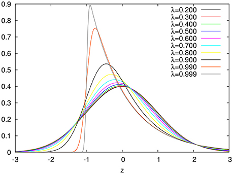
Figure 1. ex-Gaussian distributions for different values of the λ asymmetry parameter.
FIGURE 2
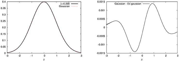
Figure 2. Differences between the ex-Gaussian distribution with λ = 0.2 and the gaussian distribution. Both curves plotted on the left and the difference on the right (note this difference is less than 1%).
Given a probability density, an important function that can be calculated from it is its cumulative distribution (its left tail), which is the result of the integral
The importance of this function is that given the cumulative distribution one is able to calculate the probability of an event. For the ex-gaussian, the expression for its cumulative distribution is given by:
Let's also define zα, the value of z for which the right tail of the distribution has an area equal to α:
so, solving the Equation (14), one is able to obtain the value of zα for any given α.
3. Fitting the Probability Distribution
We are interested in the following problem: given a dataset, to estimate the parameters μ, σ and τ that, plugged into Equation (5), best fit the data.
We must now define what it means to best fit the data. Different approaches here will result in different values for the parameters. The most trivial approach would be to say that the best parameters are those that result in the fitted ex-Gaussian distribution with the same statistical parameters: average (M), standard deviation (S) and asymmetry (K or λ). So, one can take the dataset, calculate M, S, and K and use the relations between them and the parameters μ, σ and τ:
This method of evaluating the parameters from the statistic (momenta) is know as the method of the moments as is usually the worst possible approach given the resulting bias. For instance, in some experiments, one finds the K parameter bigger than 2 (or λ > 1) and from Equation (17) one sees that, in order to have K > 2, σ cannot be a real number.
Another approach is to find the parameters that minimize the sum of the squared differences between the observed distribution and the theoretical one (least squares). In order to do that, one must, from the dataset, construct its distribution (a histogram), which requires some parametrization (dividing the whole range of observations in fixed intervals). Since a potentially arbitrary choice is made here, the results might be dependent on this choice. When analyzing data, we will study this dependency and come back to this point.
The last approach we will study is the maximum likelihood method. The function in Equation (5) is a continuous probability distribution for a random variable, which means that f(x)dx can be interpreted as the probability that a observation of the random variable will have the x value (with the infinitesimal uncertainty dx). So, given a set of N observations of the random variable, {xi}, with i = 1, 2, …, N, the likelihood is defined as the probability of such a set, given by:
The maximum likelihood method consists in finding the parameters μ, σ and τ that maximize the likelihood (or its logarithm2 ln). Note that in this approach, one directly uses the observations (data) without the need of any parametrization (histogram).
In both approaches, least squares and maximum likelihood, one has to find the extreme (maximum or minimum) of a function. The numerical algorithm implemented for this purpose is the steepest descent/ascent (descent for the minimum and ascent for the maximum). The algorithm consists in interactively changing the parameters of the function by amounts given by the gradient of the function in the parameter space until the gradient falls to zero (to a certain precision). There are other optimization methods, like the simplex (Van Zandt, 2000; Cousineau et al., 2004), which also iteratively updates the parameters (in the case of the simplex without the need to compute the gradients). We chose to implement steepest ascent in order to gain in efficiency: since one is able to evaluate the gradients, this greedy algorithm should converge faster than the sample techniques used by simplex. But in any case, both algorithms (steepest descent and simplex) should give the same results, since both search the same maximum or minimum.
4. The ExGUtils Module
ExGUtils is a python package with two modules in its 3.0 version: one purely programmed in python (pyexg) and the other programmed in C (uts). The advantage of having the functions programmed in C is speed, stability and numerical precision.
As mentioned, the package has two modules: pyexg and uts. The first one comprises all functions with source code programed in python, some of which depend on the numpy, scipy and random python packages. On the other hand, the module uts contains functions with source code programmed in C. In Table 1 one can find a complete list of all functions contained in both modules and the ones particular to each one. The source distribution of the ExGUtils module comes with a manual which explains in more detail and with examples the functions.
TABLE 1
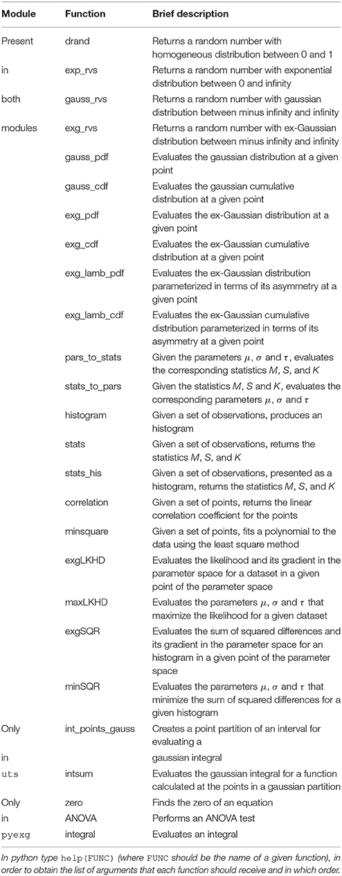
Table 1. Functions present in the package modules.
5. Applications
We use here the ExGUtils package in order to analyze data from the experiment in Navarro-Pardo et al. (2013). From this work, we analyse the datasets obtained for the reaction times of different groups of people in recognizing different sets of words in two possible experiments (yes/no and go/nogo). In the Appendix B we briefly explain the datasets analyzed here (which are provided as Supplementary Material for download).
In our analysis, first each dataset is fitted to the ex-Gaussian distribution through the three different approaches aforementioned:
• moments → Estimating the parameters through the sample statistics Equations (18–20).
• minSQR → Estimation through least square method, using as initial point in the steepest descent algorithm the μ, σ and τ obtained from the method of moments above3.
• maxLKHD → Estimation through maximum likelihood method, using as initial point in the steepest ascent algorithm the μ, σ and τ obtained from the method of moments3.
In Table 2, one can see the estimated parameters and the corresponding statistics for the different experiments. From the table, one sees that in the case of the experiments performed with young people, the value of the skewness, K, is bigger than two. This happens because of a few atypical measurements far beyond the bulk of the distribution. In fact, many researches opt for trimming extreme data, by “arbitrarly” choosing a cutoff and removing data points beyond this cutoff. One must, though, be careful for the ex-Gaussian distribution does have a long right tail, so we suggest a more criterious procedure:
TABLE 2
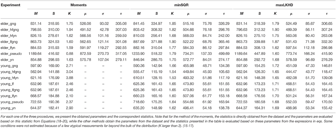
Table 2. Parameters and statistics obtained with the three fitting methods.
Having the tools developed in ExGUtils, one can use the parameters obtained in the fitting procedures (either minSQR or maxLKHD) in order to estimate a point beyond which one should find no more than, let's say, 0.1% of the distribution. In the Appendix A (Supplementary Material), the Listing 1 shows a quick python command line in order to estimate this point in the case of the young_gng experiment. The result informs us that, in principle, one should not expect to have more than 0.1% measurements of reaction times bigger than 1472.84 ms if the parameters of the distribution are the ones adjusted by maxLKHD for the young_gng empirical data. In fact, in this experiment, one has 2396 measurements of reaction times, from those, 8 are bigger than 1472.8 ms (0.33%). If one now calculates the statistics for the data, removing these 8 outliers, one obtains:
In Figure 3 one can see the histogram of data plotted along with three ex-Gaussians resulting from the above parameters.
FIGURE 3
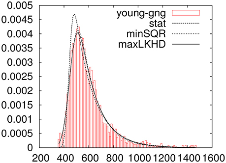
Figure 3. Data for the young_gng experiment trimmed for outliers with three fitted ex-Gaussians.
Now, one might ask, having these different fits for the same experiment, how to decide which one is the best? Accepting the parameters of a fit is the same as accepting the null hypothesis that the data measurements come from a population with an ex-Gaussian distribution with the parameters given by the ones obtained from the fit. In Clauset et al. (2009) the authors suggest a procedure in order to estimate a p-value for this hypothesis when the distribution is a power-law. One can generalize the procedure for any probability distribution, like the ex-Gaussian, for example:
• Take a measure that quantifies the distance between the data and the fitted theoretical distribution. One could use ln or χ2, but, as our fitting procedures maximize or minimize these measures, as the authors in Clauset et al. (2009) suggest, in order to avoid any possible bias, we evaluate the Kolmogorov-Smirnov statistic, which can be calculated for reaction-time data without the need of any parametrization.
• Randomly generate many data samples of the same size as the empirical one using the theoretical distribution with the parameters obtained from the fit to the empirical data.
• Fit each randomly generated data sample to the theoretical distribution using the same fit procedure used in the case of the empirical data.
• Evaluate the Kolmogorov-Smirnov statistic between the random sample and its fitted theoretical distribution.
Following this procedure, one can evaluate the probability that a random data sample, obtained from the fitted distribution, has a bigger distance to the theoretical curve than the distance between the empirical data and its fitted distribution. If this probability is higher than the confidence level one is willing to work with, one can accept the null hypothesis knowing that the probability that one is committing a type I error if one rejects the null hypothesis is p.
In the Appendix A (Supplementary Material) we provide listings with the implementation, in python via the ExGUtils package, of the functions that evaluate this p probability and the Kolmogorov-Smirnov statistic. In Table 3 we provide the values of p obtained for the experiments, using minSQR and maxLKHD approaches (p1 and p2, respectively).
TABLE 3
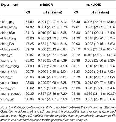
Table 3. Probabilities p1 and p2 for the fits.
We can see that there are some discrepancies in Table 3. Sometimes minSQR seems to perform better, sometimes maxLKHD. One might now remember that the minSQR method depends on a parametrization of the data. In order to perform the fit, one needs to construct a histogram of the data, and there is an arbitrary choice in the number of intervals one divides the data into. In the fits performed till now, this number is set to be the default in the histogram function of the ExGUtils package, namely two times the square root of the number of measurements in the data.
In order to study the effect of the number of intervals in the values for the parameters and of p2, we performed the procedure of fitting the data through minSQR after constructing the histogram with different number of intervals. In Figure 4 we show the evolution of the p2 probability, along with the values for μ, σ, and τ obtained by minSQR for the histograms constructed with a different number of intervals for the young_hfgng experiment.
FIGURE 4
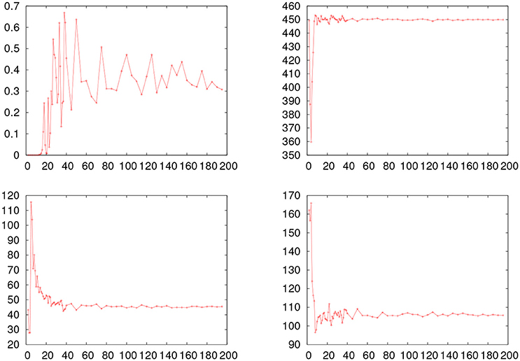
Figure 4. Fitting results obtained with the minSQR method varying the number of intervals in the histogram for the young_hfgng experiment. The horizontal line shows the value obtained with the maxLKHD method. (Upper left) Evolution of the p probability. (Upper right) Evolution of μ. (Bottom left) Evolution of σ. (Bottom right) Evolution of τ.
From the figure one sees that while the number of intervals is unreasonably small compared to the size of the empirical dataset, the values for the fitted ex-Gaussian parameters fluctuate, while the p probability is very small, but, once the number of intervals reaches a reasonable value, around 40, the values for the parameters stabilize and the value of p also gets more stable. So the question remains, why the values for the probability obtained with maxLKHD method is so small in the case of this experiment? The fact is that the likelihood of the dataset is very sensible to outliers. For the value of the probability [f(x) in Equation 5] gets very small for the extreme values. Therefore, in these cases, it might be reasonable to make some criterious data trimming. So we proceed as follows: Given a dataset, we first perform a pre-fitting by maxLKHD. Using the parameters obtained in this fit, we estimate the points where the distribution has a left and right tails of 0.1% and remove measurements beyond these points. With the trimmed dataset, removed of outliers, we perform fits again and evaluate the p1 and p2 probabilities. In Table 4, we show the results for this new round of fitting and probability evaluations. In more than half of the experiments where one could see a big discrepancy between p1 and p2 in Table 3, the trimmed data do show better results. For some datasets, the trimming had no impact on the discrepancy. In any case, one might wonder about the impact of the trimming in the obtained parameters. Therefore, in Table 5, we show the results obtained with different trimming criteria.
TABLE 4
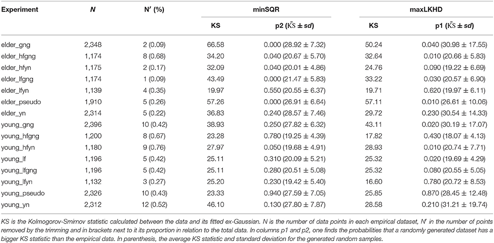
Table 4. The p1 and p2 probabilities for the fits.
TABLE 5

Table 5. Results for different trimming on the data.
Now, having the full picture, one can realize that some values of p are indeed small, indicating that either the ex-Gaussian distribution is not that good a model in order to fit the empirical results, or there is still some systematic error in the analysis of the experiments. Most of these empirical datasets where one sees very low values of p are with elderly people. These have the τ parameter much bigger than the σ which indicates a very asymmetric distribution with a long right tail. Indeed, a careful analysis of the histograms will show that the tail in these empirical distributions seems to be cut short at the extreme of the plots, so that the limit time in the experiment should be bigger than 2,500 ms in order to get the full distribution. One might argue that the trimming actually was removing data, but most of the removed points in the trimming of elderly data, was from the left tail and not from the right. This issue will result in the wrong evaluation of the KS statistics, since it assumes that one is dealing with the full distribution. This kind of analysis might guide better experimental designs.
6. Overview
The ex-Gaussian fit has turned into one of the preferable options when dealing with positive skewed distributions. This technique provides a good fit to multiple empirical data, such as reaction times (a popular variable in Psychology due to its sensibility to underlying cognitive processes). Thus, in this work we present a python package for statistical analysis of data involving this distribution.
This tool allows one to easily work with alternative strategies (fitting procedures) to some traditional analysis like trimming. This is an advantage given that an ex-Gaussian fit includes all data while trimming may result in biased statistics because of the cuts.
Moreover, this tool is programmed as Python modules, which allow the researcher to integrate them with any other Python resource available. They are also open-source and free software which allows one to develop new tools using these as building blocks.
7. Availability
ExGUtils may be downloaded from the Python Package index (https://pypi.python.org/pypi/ExGUtils/3.0) for free along with the source files and the manual with extended explanations on the functions and examples.
Author Contributions
CM-T participated in the conception, design, and interpretation of data, and in drafting the manuscript. DG participated in the design, and analysis and interpretation of data, and in drafting the manuscript. EN-P and PF participated in revising the manuscript.
Funding
This work has been financed under the Generalitat Valenciana research project GV/2016/188 (Prof. Carmen Moret-Tatay) and the Universidad Católica de Valencia, San Vicente Mártir.
Conflict of Interest Statement
The authors declare that the research was conducted in the absence of any commercial or financial relationships that could be construed as a potential conflict of interest.
Supplementary Material
The Supplementary Material for this article can be found online at: https://www.frontiersin.org/articles/10.3389/fpsyg.2018.00612/full#supplementary-material
Footnotes
1. ^In this cases, the numerical evaluation of the ex-Gaussian distribution in Equation (5) becomes unstable and one can without loss (to a precision of around one part in a million) approximate the ex-Gaussian by a gaussian distribution.
2. ^Note that, since the logarithm is an monotonically increasing function, the maximal argument will result in the maximum value of the function as well.
3. ^In the cases where K was bigger than 2, the inicial parameters were calculated as if K = 1.9. Note that the final result of the search should not depend on the inicial search point if it starts close to the local maximum/minimum.
References
Balota, D. A., Cortese, M. J., Sergent-Marshall, S. D., Spieler, D. H., and Yap, M. (2004). Visual word recognition of single-syllable words. J. Exp. Psychol. Gen. 133:283. doi: 10.1037/0096-3445.133.2.283
Clauset, A., Shalizi, C. R., and Newman, M. E. J. (2009). Power-Law distributions in empirical data. SIAM Rev. 51, 661–703. doi: 10.1137/070710111
Cousineau, D., Brown, S., and Heathcote, A. (2004). Fitting distributions using maximum likelihood: methods and packages. Behav. Res. Methods Instrum. Comput. 36, 742–756. doi: 10.3758/BF03206555
Cousineau, D., and Larochelle, S. (1997). Pastis: a program for curve and distribution analyses. Behav. Res. Methods Instrum. Comput. 29, 542–548. doi: 10.3758/BF03210606
Epstein, J. N., Langberg, J. M., Rosen, P. J., Graham, A., Narad, M. E., Antonini, T. N., et al. (2011). Evidence for higher reaction time variability for children with adhd on a range of cognitive tasks including reward and event rate manipulations. Neuropsychology 25:427. doi: 10.1037/a0022155
Gooch, D., Snowling, M. J., and Hulme, C. (2012). Reaction time variability in children with adhd symptoms and/or dyslexia. Dev. Neuropsychol. 37, 453–472. doi: 10.1080/87565641.2011.650809
Grushka, E. (1972). Characterization of exponentially modified gaussian peaks in chromatography. Anal. Chem. 44, 1733–1738. doi: 10.1021/ac60319a011
Heathcote, A. (2004). Fitting wald and ex-wald distributions to response time data: an example using functions for the s-plus package. Behav. Res. Methods Instrum. Comput. 36, 678–694. doi: 10.3758/BF03206550
Heathcote, A., Popiel, S. J., and Mewhort, D. (1991). Analysis of response time distributions: an example using the stroop task. Psychol. Bull. 109:340.
Hervey, A. S., Epstein, J. N., Curry, J. F., Tonev, S., Eugene Arnold, L., Keith Conners, C., et al. (2006). Reaction time distribution analysis of neuropsychological performance in an adhd sample. Child Neuropsychol. 12, 125–140. doi: 10.1080/09297040500499081
Lacouture, Y., and Cousineau, D. (2008). How to use matlab to fit the ex-gaussian and other probability functions to a distribution of response times. Tutor. Quant. Methods Psychol. 4, 35–45. doi: 10.20982/tqmp.04.1.p035
Leth-Steensen, C., King Elbaz, Z., and Douglas, V. I. (2000). Mean response times, variability, and skew in the responding of adhd children: a response time distributional approach. Acta Psychol. 104, 167–190. doi: 10.1016/S0001-6918(00)00019-6
Luce, R. D. (1986). Response Times: Their Role in Inferring Elementary Mental Organization. Oxford psychology series. New York, NY; Oxford: Oxford University Press; Clarendon Press.
McVay, J. C., and Kane, M. J. (2012). Drifting from slow to “D'oh!”: working memory capacity and mind wandering predict extreme reaction times and executive control errors. J. Exp. Psychol. Learn. Mem. Cogn. 38:525. doi: 10.1037/a0025896
Navarro-Pardo, E., Navarro-Prados, A. B., Gamermann, D., and Moret-Tatay, C. (2013). Differences between young and old university students on a lexical decision task: evidence through an ex-Gaussian approach. J. Gen. Psychol. 140, 251–268. doi: 10.1080/00221309.2013.817964
Ratcliff, R., Love, J., Thompson, C. A., and Opfer, J. E. (2012). Children are not like older adults: a diffusion model analysis of developmental changes in speeded responses. Child Dev. 83, 367–381. doi: 10.1111/j.1467-8624.2011.01683.x
Ratcliff, R., and McKoon, G. (2008). The diffusion decision model: theory and data for two-choice decision tasks. Neural Comput. 20, 873–922. doi: 10.1162/neco.2008.12-06-420
Sternberg, S. (1966). High-speed scanning in human memory. Science 153, 652–654. doi: 10.1126/science.153.3736.652
Van Zandt, T. (2000). How to fit a response time distribution. Psychon. Bull. Rev. 7, 424–465. doi: 10.3758/BF03214357
West, R. (1999). Age differences in lapses of intention in the stroop task. J. Gerontol. Ser. B Psychol. Sci. Soc. Sci. 54, P34–P43. doi: 10.1093/geronb/54B.1.P34
West, R., and Alain, C. (2000). Age-related decline in inhibitory control contributes to the increased stroop effect observed in older adults. Psychophysiology 37, 179–189. doi: 10.1111/1469-8986.3720179
Keywords: response times, response components, python, ex-Gaussian fit, significance testing
Citation: Moret-Tatay C, Gamermann D, Navarro-Pardo E and Fernández de Córdoba Castellá P (2018) ExGUtils: A Python Package for Statistical Analysis With the ex-Gaussian Probability Density. Front. Psychol. 9:612. doi: 10.3389/fpsyg.2018.00612
Received: 29 December 2017; Accepted: 11 April 2018;
Published: 01 May 2018.
Edited by:
Axel Hutt, German Meteorological Service, GermanyReviewed by:
Denis Cousineau, University of Ottawa, CanadaMiguel A. Vadillo, Universidad Autonoma de Madrid, Spain
Copyright © 2018 Moret-Tatay, Gamermann, Navarro-Pardo and Fernández de Córdoba Castellá. This is an open-access article distributed under the terms of the Creative Commons Attribution License (CC BY). The use, distribution or reproduction in other forums is permitted, provided the original author(s) and the copyright owner are credited and that the original publication in this journal is cited, in accordance with accepted academic practice. No use, distribution or reproduction is permitted which does not comply with these terms.
*Correspondence: Carmen Moret-Tatay, mariacarmen.moret@ucv.es