Dynamic coverage control in unicycle multi-robot networks under anisotropic sensing

1. Introduction

Mobile sensor and robotic networks have been of major research interest during the past decade, in part due to their usefulness in applications ranging from surveillance and monitoring, to situational awareness, to tasks involving industrial and domestic robots (e.g., for painting, floor cleaning, lawn mowing). A mobile sensor or robotic network is typically realized as a group of agents, which are characterized by local sensing capabilities and which need to collaborate to achieve a global objective, often addressed as coverage.

Coverage is typically classified into static coverage control and dynamic coverage control. The static coverage control problem mainly addresses the optimal placement of sensors to cover a region and reduces to finding control laws, which deploy mobile sensing agents to the centroids of Voronoi cells in a Voronoi partitioning of a given domain (Cortes et al., 2004; Cheng and Savkin, 2010; Ferrari et al., 2010; Schwager et al., 2011; Zhong and Cassandras, 2011). On the contrary, the term dynamic coverage control has traditionally been used to describe problems where a group of mobile sensing agents is deployed to search an area sufficiently well over time, see, for instance, Hokayem et al. (2007), Hussein and Stipanovic (2007), Atinç et al. (2013), and Stipanovic et al. (2013) and the references therein. The main concept, which realizes sufficient (or effective) coverage, is a parameter C^⋆, which is associated with the amount of time that a sensing agent should spend on every point of the area. One common thread in earlier work on dynamic coverage is the consideration of isotropic sensing for each agent, which is realized as a bell-shaped sensing function over a circular sensing footprint. Nevertheless, although this model is suitable for agents carrying sensors such as laser range finders, it is not pertinent for agents with onboard cameras.

This paper is in part motivated by surveillance applications where vision is the main means of sensing and information gathering and addresses dynamic coverage for multiple non-holonomic agents along with collision avoidance guarantees. We extend our earlier work (Stipanovic et al., 2013) by considering a new dynamic coverage and avoidance control design, which can be implemented in a decentralized fashion. The main difference here is the consideration of (i) anisotropic sensing, realized via conic sensing footprints and conic sensing (coverage) functions for each agent, and (ii) a novel form of avoidance functions. The considered sensing functions encode field-of-view and range constraints, and furthermore the degradation of effective sensing close to the boundaries of the sensing footprint. In this spirit, the proposed control design is suitable for surveillance tasks, where a group of robots is assigned with the task to gather enough information about an environment (such as video streaming or snapshots) locally, while avoiding collisions. More specifically, the considered scenario in this paper addresses the case of non-holonomic robots, each one carrying a forward-looking camera of limited angle-of-view and a rear proximity sensor, such as a laser scanner. Each robot is thus capable of detecting objects both in the forward and the backward looking direction, and more specifically, objects lying within the finite conic sensing footprints dictated by the available sensor limitations. The dynamic coverage control is defined as ensuring that each point of a domain of interest is sensed by the forward-looking sensing footprint of at least one agent (that is, the same point may be sensed by more than one agent) for a sufficient amount of time. A coverage error function encoding this objective is defined for each agent, and control laws, which guarantee that this error is driven to zero, are designed. The local encoding of coverage capability through the adopted error function implies that agents may stop moving before the entire domain has been sufficiently covered. For this reason, a supervisory logic is additionally implemented; this is realized as the exchange of information among agents regarding their individually covered areas, so that at least one agent has knowledge of the entire coverage map, and the selection of waypoints in the uncovered area toward, which the agents are forced to move after their individual coverage errors have become arbitrarily close to zero. The implementation for the supervisory logic is based on Atinç et al. (2013) and further refined to the conic sensing and coverage models considered here. Avoidance is considered only pairwise in this paper, and is implemented through novel avoidance functions, which are compatible with the available conic sensing footprints. Extending this encoding to multi-robot avoidance control is currently ongoing work.

The consideration of anisotropic sensors for coverage control problems has been also considered in Gusrialdi et al. (2008a,b), Laventall and Cortes (2008), and Hexsel et al. (2013); however, these contributions refer to static coverage problems, i.e., to agents covering areas in a deployment sense, and therefore are not relevant to the dynamic coverage formulation presented here. To the best of our knowledge, the most relevant work to this paper is Franco et al. (2012), which addresses vision-based dynamic coverage for mobile robots. Yet, the current paper differs in the sensing modeling, which is realized via a novel form of conical functions, as well as in the proposed coverage and avoidance control strategies, which here are based on novel coverage and avoidance functions.

A shorter version of this paper appeared in Panagou et al. (2014). The current version includes the complete technical analysis on the considered control design, which is omitted in the conference version in the interest of space, and additionally presents a way of addressing the “global” coverage objective via a supervisory logic, which eliminates the limitations of the “local” dynamic coverage control design. The difference between global and local coverage will become clear in later sections.

The paper is organized as follows: Section 2.1 describes the system modeling along with the sensing constraints and functions. Sections 2.2 and 2.3 include the novel formulations regarding the (local) coverage and collision avoidance control, while the technical analysis on the proposed control strategies is presented in Section 2.3.3. Simulation results are reported in Section 3, along with a way of addressing the global coverage objective. Section 4 summarizes our results and thoughts on future research, followed by some pertinent acknowledgments.

2. Materials and Methods

2.1. Problem Formulation

Consider a group of N mobile agents, whose motion is governed by unicycle kinematics:

$\left[\begin{array}{c}\hfill {\dot{x}}_i\hfill \\ \hfill {\dot{y}}_i\hfill \\ \hfill {\dot{\mathrm{\theta }}}_i\hfill \end{array}\right]=\left[\begin{array}{cc}\hfill \cos {\mathrm{\theta }}_i\hfill & \hfill 0\hfill \\ \hfill \sin {\mathrm{\theta }}_i\hfill & \hfill 0\hfill \\ \hfill 0\hfill & \hfill 1\hfill \end{array}\right]\left[\begin{array}{c}\hfill u_i\hfill \\ \hfill {\mathrm{\omega }}_i\hfill \end{array}\right],$ (1)

where i ∈{1, $\dots$, N}, p_i = [x_i y_i]^T is the position vector and θ_i is the orientation of an agent i (w.r.t) a global coordinate frame $\mathcal{G}$, and u_i, ω_i are the linear and angular velocities of agent i, respectively (w.r.t), the body frame ${\mathcal{B}}_i$. Denote $q_i={\left[\begin{array}{cc}\hfill p_i^T\hfill & \hfill {\mathrm{\theta }}_i\hfill \end{array}\right]}^T$ the state vector of agent i.

Each agent is assumed to be equipped with a fixed onboard camera of limited angle-of-view and furthermore to be able to detect objects, which lie within a limited region (w.r.t) the forward-looking direction. The limited sensing region of agent i is realized as a circular sector ${\mathcal{S}}_i$ of angle 2α_i and radius R_i, where R_i > 0, α_i ∈ (0, π/2) (Figure 1).

FIGURE 1

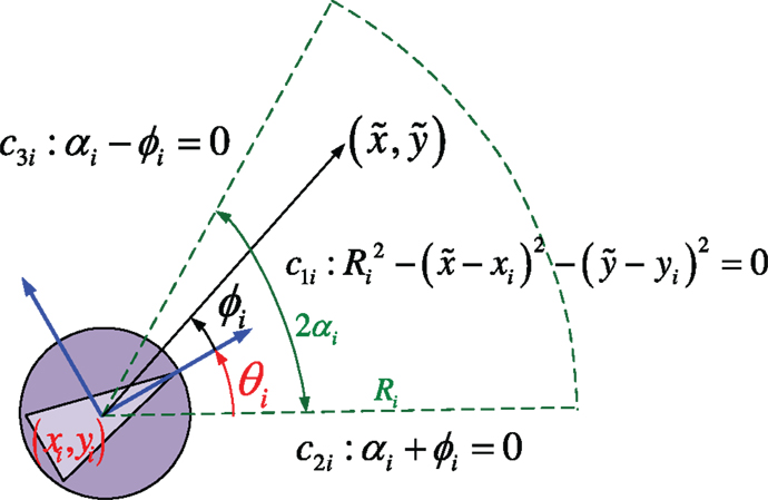
Figure 1. The forward-looking sensing footprint ${\mathcal{S}}_i$ for agent i.

Furthermore, each agent is assumed to have a rear proximity sensor, whose sensing footprint ${\mathcal{S}}_i^{\prime }$ is for simplicity modeled as the symmetric circular sector of ${\mathcal{S}}_i$ (w.r.t) the $y_{{\mathcal{B}}_i}$ body-fixed axis of agent i. In that respect, each agent i is able to detect objects lying within a limited range in the backward direction as well. The role of the rear proximity sensor is to ensure that each agent i is able to detect and avoid objects (obstacles and other agents j ≠ i) when forced to move backwards.

2.1.1. Modeling of conic sensing footprints

Consider the functions $c_{ki}:{\mathbb{R}}^3\to \mathbb{R}$ defined as:

$c_{1i}\left(t\right)=R_i^2-{\left({\tilde{x}}_i-x_i\left(t\right)\right)}^2-{\left({\tilde{y}}_i-y_i\left(t\right)\right)}^2,$ (2a)

$c_{2i}\left(t\right)={\mathrm{\alpha }}_i-{\mathrm{\varphi }}_i\left(t\right),$ (2b)

$c_{3i}\left(t\right)={\mathrm{\alpha }}_i+{\mathrm{\varphi }}_i\left(t\right),$ (2c)

where k ∈ {1, 2, 3}, $\tilde{p}={\left[\begin{array}{cc}\hfill \tilde{x}\hfill & \tilde{y}\end{array}\right]}^T$ is the position vector of a point on ${\mathbb{R}}^2$, p_i(t) = [x_i(t) y_i(t)]^T is the position vector, and θ_i(t) is the orientation of agent i at time instant t, and

${\mathrm{\varphi }}_i\left(t\right)=\text{atan}2\left({\tilde{y}}_i-y_i\left(t\right),{\tilde{x}}_i-x_i\left(t\right)\right)-{\mathrm{\theta }}_i\left(t\right)$ (3)

is the angle of a point $\tilde{p}\in R^2$ (w.r.t) the body frame B_i of agent i at time instant t. The region of the state space where all functions equation (2) take non-negative values encode a circular sector ${\mathcal{S}}_i$ of radius R_i and angle 2α_i centered at p_i(t). This circular sector models the forward-looking sensing footprint for agent i (Figure 1). For simplicity, in the sequel, we assume that all agents have the same sensing capabilities, i.e., that R_i = R, α_i = α.

Let us now note that the barrier function:

$B_i=\frac{1}{\max \left\{0,c_{1i}\right\}}+\frac{1}{\max \left\{0,c_{2i}\right\}}+\frac{1}{\max \left\{0,c_{3i}\right\}}$

tends to +∞ as the k-th constraint c_ki → 0⁺, i.e., as a point $\tilde{p}$ on the interior of the set ${\mathcal{S}}_i$ approaches the boundary $\partial {\mathcal{S}}_i$ of ${\mathcal{S}}_i$. To keep notation compact, denote max{0, c_ki} = C_ki, k ∈ {1, 2, 3}, and consider the function:

$S_i=\frac{1}{B_i}=\frac{C_{1i}{C}_{2i}{C}_{3i}}{C_{2i}{C}_{3i}+C_{1i}{C}_{3i}+C_{1i}{C}_{2i}},$ (4)

which is zero on the exterior of the sensing footprint ${\mathcal{S}}_i$, zero on the boundary $\partial {\mathcal{S}}_i$ except for at the points where any two of the constraints c_ki are concurrently zero, and positive on the interior of ${\mathcal{S}}_i$. Furthermore, equation (4) tends to zero as the k-th constraint c_ki → 0⁺ (Figure 2). We define that the sensing function ${\mathcal{S}}_i$ is zero at the points where any two of the constraints are active at the same time.

FIGURE 2

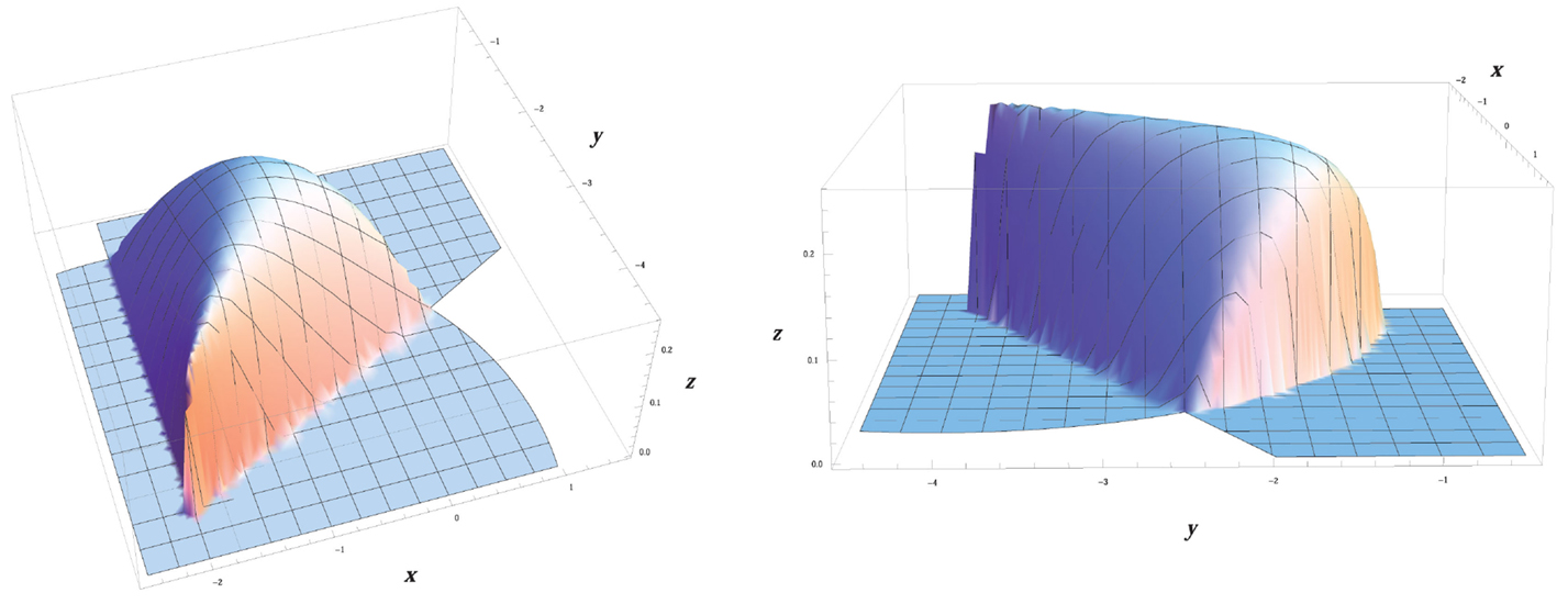
Figure 2. The considered sensing model S_i(t) for agent i, given by equation (9). The agent is positioned at p_i = | − 2 − 4|^T and its orientation is θ_i = π/3.

In this respect, the function S_i can be used as a realistic modeling of the available sensing capability, in the sense that the quality of sensing typically degrades as an object lies far from the camera or close to the boundaries of the camera angle-of-view. In other words, the function S_i encodes that sensing of objects (or, in other words, “seeing”) becomes less effective as these lie closer to the boundaries of the sensing footprint ${\mathcal{S}}_i$ of agent i.

Following our earlier work (Stipanovic et al., 2013), the sensing function for the i-th agent is defined:

$Q_i\left(t,\tilde{p}\right)={\int }_0^t{S}_i\left(p_i\left(\mathrm{\tau }\right),{\mathrm{\theta }}_i\left(\mathrm{\tau }\right),\tilde{p}\right)d\mathrm{\tau }.$ (5)

Let us also define the function h(w) = (max{0, w})³, so that its first derivative reads: h′ = dh/dw = 3(max{0, w})², and its second derivative reads: h″ = d²h/dw² = 6(max{0, w}).

2.2. Coverage Control

Given a compact region D, we are interested in deriving control strategies, which guarantee that the agents cover (or search) the whole region up to a satisfactory level. In other words, the term satisfactory coverage denotes that each point $\tilde{p}$ of D should be sensed by at least one agent for a sufficient amount of time. In order to mathematically capture the notion of satisfactory coverage, we use a positive constant C^⋆. The value of this constant is chosen depending on how well we would like to search the area; more specifically, larger values of C^⋆ are meant to force each agent to spend more time sensing each point on the domain.

2.2.1. Coverage error function

The coverage error for the i-th agent is defined as:

$e_i\left(t\right)=\underset{D}{\int }h\left(C^{\star }-Q_i\left(t,\tilde{p}\right)\right)d\tilde{p},$ (6)

where D is the compact region to be covered and C^⋆ is the positive constant realizing the satisfactory coverage level. A meaningful choice of the value C^⋆ is to pick C^⋆ ≥ t max S_i, where t is the least amount of time that an agent needs to spend on each point $\tilde{p}$ of the domain D and max S_i is the maximum value of the sensing function equation (4). The time derivative of equation (6) reads:

${ė}_i\left(t\right)=-\underset{D}{\int }h\prime \left(C^{\star }-Q_i\left(t,\tilde{p}\right)\right)S_i\left(p_i\left(t,\tilde{p}\right),{\mathrm{\theta }}_i\left(t\right)\right)d\tilde{p}.$ (7)

Remark 1. In general, the derivative of the area integral

$J\left(t\right)={\displaystyle \underset{D\left(t\right)}{\iint }}f\left(t,\tilde{x},\tilde{y}\right)d\tilde{x}d\tilde{y}$

of a function $f\left(t,\tilde{x},\tilde{y}\right)$ over a compact region D(t), which is bounded by a closed curve C(t), which is continuous and consists of smooth arcs, is given as:

$\frac{\mathit{dJ}\left(t\right)}{\mathit{dt}}=\underset{D\left(t\right)}{\iint }\frac{\mathrm{\partial }f\left(t,\tilde{x},\tilde{y}\right)}{\mathrm{\partial t}}d\tilde{x}d\tilde{y}+I\left(t\right),$

where:

$I\left(t\right)=\underset{C\left(t\right)}{\oint }f\left(t,\tilde{x},\tilde{y}\right)\left(\frac{\partial \tilde{x}}{\mathit{dt}}d\tilde{y}-\frac{\partial \tilde{y}}{\mathit{dt}}d\tilde{x}\right),$

with the integration performed along the counterclockwise direction. It can be shown that for the considered sensing function ${\mathcal{Q}}_i\left(t,\tilde{x},\tilde{y}\right),$ which is exactly zero almost everywhere on the boundary C(t), the term I(t) is zero. This justifies why the term involving the line integral has been dropped in equation (7). The same holds later on for the time derivative equation (9) of the modified error function equation (8).

As discussed in Stipanovic et al. (2013), the use of equation (7) as a candidate Lyapunov-like function for guaranteeing the accomplishment of satisfactory coverage is not a good choice, in the sense that this function may become zero when the S_i(⋅) term becomes zero, and this condition may occur, for instance, when agent i leaves the domain D. Thus, the following modified error function is utilized instead as a Lyapunov-like function:

${ê}_i\left(t\right)=-\underset{D}{\int }h\prime \left(C^{\star }-Q_i\left(t,q_i,\tilde{p}\right)\right)\left(S^{\star }-S_i\left(p_i\left(t,\tilde{p}\right),{\mathrm{\theta }}_i\left(t\right)\right)\right)d\tilde{p},$ (8)

where S^⋆ > N max S_i a positive constant; this functional is negative and vanishes when the term $h\prime \left(C^{\star }-Q_i\left(t,q_i,\tilde{p}\right)\right)$ becomes zero, i.e., only when the satisfactory coverage level C^⋆ for a point $\tilde{p}\in D$ has been achieved. The time derivative of equation (8) reads as in equation (9),

$\begin{array}{llll}\hfill {\dot{ê}}_i\left(t\right)& =-\underset{D}{\int }\left(-h″\left(C^{\star }-Q_i\left(t,\tilde{p}\right)\right)S_i\left(p_i\left(t,\tilde{p}\right),{\mathrm{\theta }}_i\left(t\right)\right)\times \left(S^{\star }-S_i\left(p_i\left(t,\tilde{p}\right),{\mathrm{\theta }}_i\left(t\right)\right)\right)-h\prime \left(C^{\star }-Q_i\left(t,\tilde{p}\right)\right)\right.& \hfill & \\ \hfill & \left.\times \frac{d}{\mathit{dt}}\left(S_{i}l\left(p_i\left(t,\tilde{p}\right),{\mathrm{\theta }}_i\left(t\right)\right)\right)\right)d\tilde{p}\\ \hfill & =\underset{D}{\int }\left(h″\left(C^{\star }-Q_i\left(t,\tilde{p}\right)\right)S_i\left(p_i\left(t,\tilde{p}\right),{\mathrm{\theta }}_i\left(t\right)\right)\right.\times \left(S^{\star }-S_i\left(p_i\left(t,\tilde{p}\right),{\mathrm{\theta }}_i\left(t\right)\right)\right)+h\prime \left(C^{\star }-Q_i\left(t,\tilde{p}\right)\right)& \hfill & \\ \hfill & \left.\times \frac{d}{\mathit{dt}}\left(S_i\left(p_i\left(t,\tilde{p}\right),{\mathrm{\theta }}_i\left(t\right)\right)\right)\right)d\tilde{p}& \hfill & \\ \hfill & =\underset{D}{\int }h″\left(C^{\star }-Q_i\left(t,\tilde{p}\right)\right)S_i\left(p_i\left(t,\tilde{p}\right),{\mathrm{\theta }}_i\left(t\right)\right)\times \left(S^{\star }-S_i\left(p_i\left(t,\tilde{p}\right),{\mathrm{\theta }}_i\left(t\right)\right)\right)d\tilde{p}& \hfill & \\ \hfill & +\underset{D}{\int }h\prime \left(C^{\star }-Q_i\left(t,\tilde{p}\right)\right)\frac{d}{\mathit{dt}}\left(S_i\left(p_i\left(t,\tilde{p}\right),{\mathrm{\theta }}_i\left(t\right)\right)\right)d\tilde{p},\end{array}$ (9)

$\begin{array}{ll}\hfill & \mathrm{where\; :}\frac{d}{\mathit{dt}}\left(S_i\left(p_i\left(t,\tilde{p}\right),{\mathrm{\theta }}_i\left(t\right)\right)\right)=\frac{\partial S_i}{\partial x_i}{\dot{x}}_i\left(t\right)+\frac{\partial S_i}{\partial y_i}{\dot{y}}_i\left(t\right)+\frac{\partial S_i}{\partial {\mathrm{\theta }}_i}{\dot{\mathrm{\theta }}}_i\left(t\right)\underset{=}{\left(1\right)}\left(\frac{\partial S_i}{\partial x_i}\cos {\mathrm{\theta }}_i\left(t\right)+\frac{\partial S_i}{\partial y_i}\sin {\mathrm{\theta }}_i\left(t\right)\right)u_i\left(t\right)\\ \hfill & +\frac{\partial S_i}{\partial {\mathrm{\theta }}_i}{\mathrm{\omega }}_i\left(t\right).& \hfill & \end{array}$

and is further rewritten as:

${\dot{ê}}_i\left(t\right)=a_0\left(t\right)+u_i\left(t\right)a_1\left(t\right)+{\mathrm{\omega }}_i\left(t\right)a_2\left(t\right),$ (10)

where:

$\begin{array}{llll}\hfill a_0\left(t\right)& =\underset{D}{\int }h″\left(C^{\star }-Q_i\left(t,\tilde{p}\right)\right)S_i\left(p_i\left(t,\tilde{p}\right),{\mathrm{\theta }}_i\left(t\right)\right)\times \left(S^{\star }-S_i\left(p_i\left(t,\tilde{p}\right),{\mathrm{\theta }}_i\left(t\right)\right)\right)d\tilde{p},& \hfill & \\ \hfill a_1\left(t\right)& =\underset{D}{\int }h\prime \left(C^{\star }-Q_i\left(t,\tilde{p}\right)\right)\times \left(\frac{\partial S_i}{\partial x_i}\cos {\mathrm{\theta }}_i\left(t\right)+\frac{\partial S_i}{\partial y_i}\sin {\mathrm{\theta }}_i\left(t\right)\right)d\tilde{p},& \hfill & \\ \hfill a_2\left(t\right)& =\underset{D}{\int }h\prime \left(C^{\star }-Q_i\left(t,\tilde{p}\right)\right)\frac{\partial S_i}{\partial {\mathrm{\theta }}_i}d\tilde{p}.& \hfill & \end{array}$

As the functional equation (8) is non-positive, it follows that for the error ${ê}_i\left(t\right)$ converging to zero, it suffices that its time derivative ${\dot{ê}}_i\left(t\right)$ is non-negative (Stipanovic et al., 2013).

Theorem 1. If agent i moves under the control law:

$\begin{array}{ll}\hfill u_i^{\mathit{cov}}& =k_u^{\mathit{cov}}\underset{D}{\int }\underset{\mathrm{\mu }\left(\cdot \right)}{\underbrace{h\prime \left(C^{\star }-Q_i\left(t,\tilde{p}\right)\right)\left(\frac{\partial S_i}{\partial x_i}\cos {\mathrm{\theta }}_i+\frac{\partial S_i}{\partial y_i}\sin {\mathrm{\theta }}_i\right)}}d\tilde{p},\end{array}$ (11a)

$\begin{array}{ll}\hfill {\mathrm{\omega }}_i^{\mathit{cov}}& =k_{\mathrm{\omega }}^{\mathit{cov}}\underset{D}{\int }\underset{\mathrm{\nu }\left(\cdot \right)}{\underbrace{h\prime \left(C^{\star }-Q_i\left(t,\tilde{p}\right)\right)\frac{\partial S_i}{\partial {\mathrm{\theta }}_i}}}d\tilde{p},\end{array}$ (11b)

where $k_u^{\mathit{cov}},k_{\mathrm{\omega }}^{\mathit{cov}}>0,$ then the modified coverage error equation (8) converges to zero. This in turn implies that the coverage error e_i(t) defined by equation (6) converges to zero.

Proof. Under the control law equation (11), the time derivative equation (10) of the modified error function equation (8) is non-negative; as explained earlier, this implies that equation (8) is non-decreasing.

Denote int(${\mathcal{S}}_i$) the interior of the set ${\mathcal{S}}_i$, $\partial {\mathcal{S}}_i$ the boundary of the set ${\mathcal{S}}_i$, ${\overline{\mathcal{S}}}_i=\mathrm{int(}{\mathcal{S}}_i\mathrm{)}\bigcup \partial {\mathcal{S}}_i$ the closure of the set ${\mathcal{S}}_i$, and $\mathrm{ext}\left({\mathcal{S}}_i\right)=D\setminus {\overline{\mathcal{S}}}_i$ the exterior of the set ${\mathcal{S}}_i$. Since $D=\text{int}\left({\mathcal{S}}_i\right)\mathrm{\cup }\partial {\mathcal{S}}_i\mathrm{\cup }\text{ext}\left({\mathcal{S}}_i\right)$, one has:

$\begin{array}{llll}\hfill & \underset{D}{\int }\mathrm{\mu }\left(\cdot \right)d\tilde{p}=\underset{\partial {\mathcal{S}}_i\bigcup \mathrm{ext}\left({\mathcal{S}}_i\right)}{\int }\mathrm{\mu }\left(\cdot \right)d\tilde{p}+\underset{\mathrm{int}\left({\mathcal{S}}_i\right)}{\int }\mathrm{\mu }\left(\cdot \right)d\tilde{p}\stackrel{\frac{\partial S_i}{\partial x_i}=\frac{\partial S_i}{\partial y_i}=0\text{on}\partial {\mathcal{S}}_i\bigcup \mathrm{ext}\left({\mathcal{S}}_i\right)}{\Rightarrow }\underset{D}{\int }\mathrm{\mu }\left(\cdot \right)d\tilde{p}=\underset{\mathrm{int}\left({\mathcal{S}}_i\right)}{\int }\mathrm{\mu }\left(\cdot \right)d\tilde{p},& \hfill & \\ \hfill & \underset{D}{\int }\mathrm{\nu }\left(\cdot \right)d\tilde{p}=\underset{\partial {\mathcal{S}}_i\bigcup \mathrm{ext}\left({\mathcal{S}}_i\right)}{\int }\mathrm{\nu }\left(\cdot \right)d\tilde{p}+\underset{\mathrm{int}\left({\mathcal{S}}_i\right)}{\int }\mathrm{\nu }\left(\cdot \right)d\tilde{p}\stackrel{\frac{\partial S_i}{\partial {\mathrm{\theta }}_i}=0\text{on}\partial {\mathcal{S}}_i\bigcup \mathrm{ext}\left({\mathcal{S}}_i\right)}{\Rightarrow }\underset{D}{\int }\mathrm{\nu }\left(\cdot \right)d\tilde{p}=\underset{\mathrm{int}\left({\mathcal{S}}_i\right)}{\int }\mathrm{\nu }\left(\cdot \right)d\tilde{p}.\end{array}$

Thus, the control inputs equations (11a) and (11b) vanish on the set

$\mathcal{P}=\left\{\tilde{p}\in \mathrm{int}\left({\mathcal{S}}_i\right)|\left\{\underset{\mathrm{int}\left({\mathcal{S}}_i\right)}{\int }\mathrm{\mu }\left(\cdot \right)d\tilde{p}=0\right\}\right.\left.\bigcap \left\{\underset{\mathrm{int}\left({\mathcal{S}}_i\right)}{\int }\mathrm{\nu }\left(\cdot \right)d\tilde{p}=0\right\}\right\},$

which further reads that the control inputs equations (11a) and (11b) vanish on the set $\mathcal{P}\mathrm{=}{\mathcal{P}}_1\mathrm{\cup }{\mathcal{P}}_2$, where:

$\begin{array}{llll}\hfill {\mathcal{P}}_1& =\left\{\tilde{p}\in \mathrm{int}\left({\mathcal{S}}_i\right)|h\prime \left(C^{\star }-Q_i\left(t,\tilde{p}\right)\right)=0\right\},& \hfill & \\ \hfill {\mathcal{P}}_2& =\left\{\tilde{p}\in \mathrm{int}\left({\mathcal{S}}_i\right)|\left(\frac{\partial S_i}{\partial {\mathrm{\theta }}_i}=0\right)\right.\left.\bigcap \left(\frac{\partial S_i}{\partial x_i}\cos {\mathrm{\theta }}_i+\frac{\partial S_i}{\partial y_i}\sin {\mathrm{\theta }}_i=0\right)\right\}.& \hfill & \end{array}$

The set ${\mathcal{P}}_1$ reads:

${\mathcal{P}}_1=\left\{\tilde{p}\in \mathrm{int}\left({\mathcal{S}}_i\right)|{\left(\max \left\{0,C^{\star }-Q_i\left(t,\tilde{p}\right)\right\}\right)}^2=0\right\}\Rightarrow {\mathcal{P}}_1=\left\{\tilde{p}\in \mathrm{int}\left({\mathcal{S}}_i\right)|Q_i\left(t,\tilde{p}\right)\ge C^{\star }\right\}.$

This further reads that the control law equation (11) vanishes on the set $\mathcal{P}$₁, which contains the points $\tilde{p}\in \mathrm{int}\left({\mathcal{S}}_i\right)$ for which the effective coverage level C^⋆ has been reached, or equivalently that the control law equation (11) vanishes when the coverage error equation (6) becomes zero.

Remark 2. This physically means that agent i does not stop moving $(u_i^{\mathit{cov}}\left(t\right)\ne 0,{\mathrm{\omega }}_i{\left(t\right)}^{\mathit{cov}}\ne 0)$ unless at some time t it holds that all the points $\tilde{p}\in \mathrm{int}\left({\mathcal{S}}_i\left(t\right)\right)$, which are contained in the interior of the sensing footprint ${\mathcal{S}}_i$ at time t have been effectively covered.

Let us now consider the set $\mathcal{P}$₂. The first condition in $\mathcal{P}$₂ reduces to the set

${\mathcal{A}}_i=\left\{\tilde{p}\in \mathrm{int}\left({\mathcal{S}}_i\right)|{\mathrm{\varphi }}_i=0\right\}.$

Furthermore, the concurrent satisfaction of the second condition reduces to the subset of A_i described as

${\mathcal{O}}_i=\left\{\tilde{p}\in {\mathcal{A}}_i|\frac{\partial S_i}{\partial p_i}\left[\begin{array}{c}\hfill \cos {\mathrm{\theta }}_i\hfill \\ \hfill \sin {\mathrm{\theta }}_i\hfill \end{array}\right]=0\right\},$

where $\frac{\partial S_i}{\partial p_i}=\left[\frac{\partial S_i}{\partial x_i}\frac{\partial S_i}{\partial y_i}\right]$. Geometrically, this condition describes the set of points $\tilde{p}\in A_i$ where the gradient vector ∂S_i/∂p_i is orthogonal to the body-fixed axis $x_{B_i}$ of agent i, or the set of points $\tilde{p}\in \mathit{al}{A}_i$ where ∂S_i/∂p_i = 0. Let us take the analytical expression of the gradient vector ∂S_i/∂p_i evaluated at the points $\tilde{p}\in {\mathcal{A}}_i,$ that is, for ϕ_i = 0, which reads $\frac{\partial S_i}{\partial p_i}{|}_{\tilde{p}\in {\mathcal{A}}_i}=-\frac{2}{{\left(\frac{2c_{1i}}{\mathrm{\alpha }}+1\right)}^2}{\left(\tilde{p}-p_i\right)}^T$. This implies that ∂S_i/∂p_i ≠ 0 on the set A_i (recall that the point $\tilde{p}=p_i$ belongs to the boundary $\partial {\mathcal{S}}_i$, i.e., not the interior $\text{int}\left({\mathcal{S}}_i\right)$ of the set ${\mathcal{S}}_i$), and furthermore that the gradient ∂S_i/∂p_i on ${\mathcal{A}}_i$ is co-linear with, i.e., can not be orthogonal to, the body-fixed axis $x_{B_i}$. Consequently, one has that ${\mathcal{O}}_i=\mathrm{\varnothing }$, which implies that ${\mathcal{P}}_2=\mathrm{\varnothing }$, hence $\mathcal{P}={\mathcal{P}}_1$. Thus, the control law equation (11) ensures that the coverage error e_i(t) equation (6) converges to zero, which furthermore reads that the agent does not stop moving before all the points $\tilde{p}\in \mathrm{int}\left(S_i\left(t\right)\right)$ have been effectively covered. This completes the proof.

Remark 3. The coverage error e_i(t) equation (6) encodes whether agent i has effectively covered the area included in the sensing footprint ${\mathcal{S}}_i\left(t\right)$ only, i.e., it does not provide any measure on whether the entire domain D has been effectively covered. Furthermore, the control law equation (11) vanishes when all the points $\tilde{p}\in \mathrm{int}\left({\mathcal{S}}_i\left(t\right)\right)$ have been effectively covered, which means that the agent stops moving before the entire domain D has necessarily been covered. Coverage of the entire area requires the use of a supervisory logic, which is presented in Section 3.

Remark 4. The control law equation (11) depends on the current state $q_i\left(t\right)={\left[\begin{array}{cc}\hfill p_i^T\left(t\right)\hfill & \hfill {\mathrm{\theta }}_i\left(t\right)\hfill \end{array}\right]}^T$ of each agent i, only. In other words, it requires information, which is locally available to each agent i, and as thus it can be implemented in a decentralized fashion.

2.3. Avoidance Control

The safety requirement for the robotic network dictates that each agent i should avoid collisions with any other agent j ≠ i, where i, j ∈ {1, $\dots$, N}, and with any physical static obstacles in the domain D.

2.3.1. Avoidance functions

The avoidance control between agents i and j has been encoded in Stipanovic et al. (2013) via functions of the form:

$v_{\mathit{ij}}={\left(\min \left\{0,\frac{{\left(x_i-x_j\right)}^2+{\left(y_i-y_j\right)}^2-R_{ij}{}^2}{{\left(x_i-x_j\right)}^2+{\left(y_i-y_j\right)}^2-r_{\mathit{ij}}{}^2}\right\}\right)}^2,$ (12)

where R_ij > r_ij > 0. These functions’ development was motivated by the concept of avoidance control, which was introduced and further developed by Leitmann and Skowronski (1977, 1983), Leitmann (1980), Corless et al. (1987), and Corless and Leitmann (1989). The function equation (12) encodes:

(i) a safety circular region of radius r_ij centered at the position p_i = [x_i y_i]^T of agent i, in which agent j should never enter, and

(ii) a detection circular region of radius R_ij centered at p_i = [x_i y_i]^T, which models the footprint of sensors such as omni directional laser scanners or range finders.

In the sequel, it is considered that all agents have homogenous detection and safety regions, i.e., R_ij = R, r_ij = r, $\forall i,j\in \left\{1,\dots ,N\right\}$. Define the vector p_ij : = p_i − p_j and denote with ||⋅|| the standard Euclidean norm. The function v_ij is zero for ||p_ij|| > R, i.e., when agent j lies out of the detection region of agent i, and tends to +∞ as ||p_ij|| tends to r, i.e., as agent j tends to the safety region of agent i. For reasons that will become clear later on, we consider the scaled function:

$V_{\mathit{ij}}=1-e^{-v_{\mathit{ij}}},$ (13)

so that V_ij takes its values in the interval (0,1), see also Figure 3.

FIGURE 3

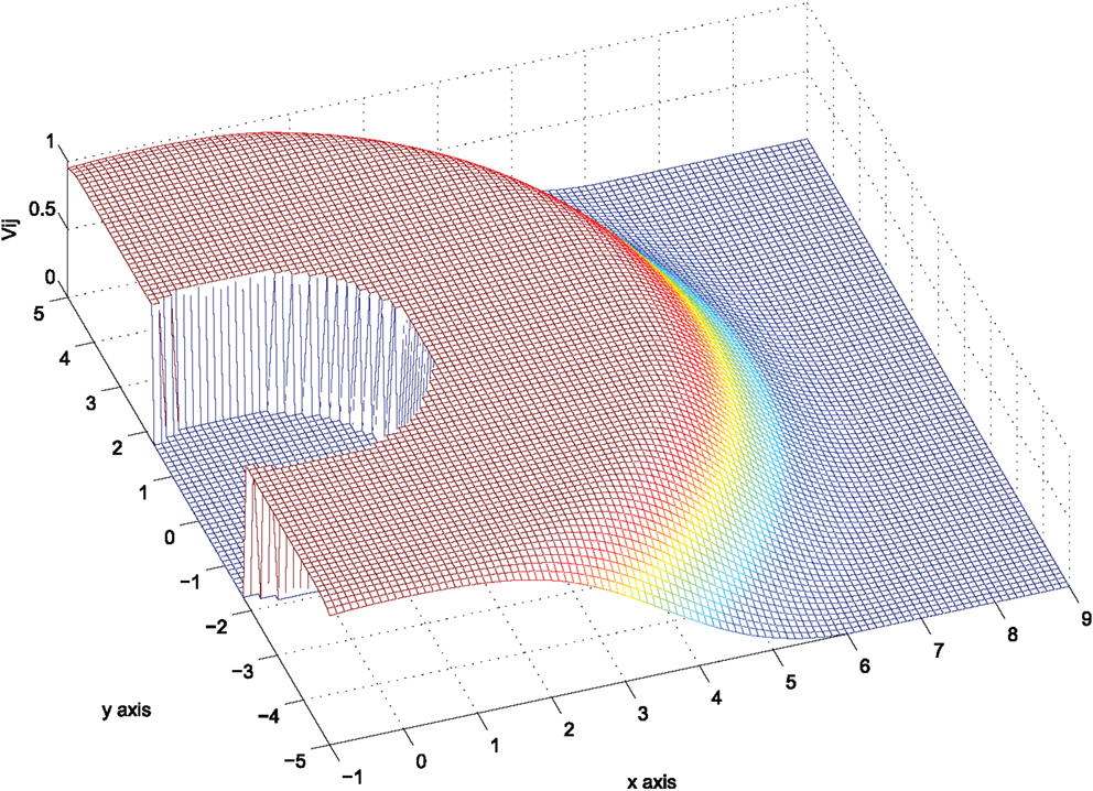
Figure 3. The avoidance function V_ij given by equation (13).

The gradient $\frac{\partial v_{\mathit{ij}}}{\partial q_i}=\left[\begin{array}{ccc}\hfill \frac{\partial v_{\mathit{ij}}}{\partial x_i}\hfill & \hfill \frac{\partial v_{\mathit{ij}}}{\partial y_i}\hfill & \hfill \frac{\partial v_{\mathit{ij}}}{\partial {\mathrm{\theta }}_i}\hfill \end{array}\right]$ of equation (12) (w.r.t), the state vector $q_i={\left[\begin{array}{cc}\hfill p_i^T\hfill & \hfill {\mathrm{\theta }}_i\hfill \end{array}\right]}^T$ reads:

$\frac{\partial v_{\mathit{ij}}}{\partial q_i}=\left\{\begin{array}{cc}\left[\begin{array}{ccc}\hfill 0\hfill & \hfill 0\hfill & \hfill 0\hfill \end{array}\right],\hfill & \mathrm{if}∥p_{\mathit{ij}}∥\ge R;\hfill \\ {\mathrm{\Omega }}_{\mathit{ij}}\left[\begin{array}{ccc}\hfill x_{\mathit{ij}}\hfill & \hfill y_{\mathit{ij}}\hfill & \hfill 0\hfill \end{array}\right],\hfill & \mathrm{if}r<∥p_{\mathit{ij}}∥<R;\hfill \\ \mathrm{not}\mathrm{defined},\hfill & \mathrm{if}∥p_{\mathit{ij}}∥=r;\hfill \\ \left[\begin{array}{ccc}\hfill 0\hfill & \hfill 0\hfill & \hfill 0\hfill \end{array}\right],\hfill & \mathrm{elsewhere},\hfill \end{array}\right.$ (14)

whereas the gradient $\frac{\partial v_{\mathit{ij}}}{\partial q_j}=\left[\begin{array}{ccc}\hfill \frac{\partial v_{\mathit{ij}}}{\partial x_j}\hfill & \hfill \frac{\partial v_{\mathit{ij}}}{\partial y_j}\hfill & \hfill \frac{\partial v_{\mathit{ij}}}{\partial {\mathrm{\theta }}_j}\hfill \end{array}\right]$ of equation (12) (w.r.t), the state vector $q_j={\left[p_j^T{\mathrm{\theta }}_j\right]}^T$ reads:

$\frac{\partial v_{\mathit{ij}}}{\partial q_j}=\left\{\begin{array}{cc}\left[\begin{array}{ccc}\hfill 0\hfill & \hfill 0\hfill & \hfill 0\hfill \end{array}\right],\hfill & \mathrm{if}∥p_{\mathit{ij}}∥\ge R;\hfill \\ -{\mathrm{\Omega }}_{\mathit{ij}}\left[\begin{array}{ccc}\hfill x_{\mathit{ij}}\hfill & \hfill y_{\mathit{ij}}\hfill & \hfill 0\hfill \end{array}\right],\hfill & \mathrm{if}r<∥p_{\mathit{ij}}∥<R;\hfill \\ \mathrm{not}\mathrm{defined},\hfill & \mathrm{if}∥p_{\mathit{ij}}∥=r;\hfill \\ \left[\begin{array}{ccc}\hfill 0\hfill & \hfill 0\hfill & \hfill 0\hfill \end{array}\right],\hfill & \mathrm{elsewhere},\hfill \end{array}\right.$

$x_{\mathit{ij}}=x_i-x_j,y_{\mathit{ij}}=y_i-y_j,{\mathrm{\Omega }}_{\mathit{ij}}=\frac{4\left(R^2-r^2\right)\left(\left|\right|p_{\mathit{ij}}|{|}^2-R^2\right)}{{\left(\left|\right|p_{\mathit{ij}}|{|}^2-r^2\right)}^3}$. Let us note that:

$\frac{\partial v_{\mathit{ij}}}{\partial q_i}=-\frac{\partial v_{\mathit{ij}}}{\partial q_j}.$ (15)

2.3.2. Encoding collision avoidance

Avoiding collisions should be encoded in a way consistent with the available sensing constraints. Each agent i is assumed to be capable of detecting objects (static obstacles and other agents j ≠ i), which lie in its sensing area ${\mathcal{S}}_i$ and therefore the motion of agent i should be collision-free (w.r.t) any object lying within ${\mathcal{S}}_i$ (Figure 4).

FIGURE 4

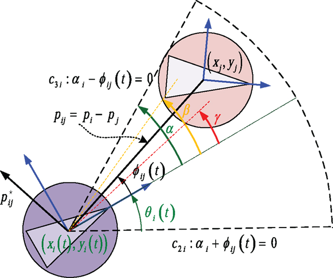
Figure 4. An agent j is effectively sensed by agent i only when it enters in the sensing area ${\mathcal{S}}_i$ of agenti.

To this end, we not only need to encode that an agent i should keep a safe distance ||p_ij|| ≥ r (w.r.t) an agent j ≠ i but also to encode that this requirement takes effect only for agents j lying in the sensing area ${\mathcal{S}}_i$ of agent i. Assume that an agent j has entered the region ${\mathcal{S}}_i$. The active constraint function c_{3 i}: α − ϕ_ij(t) = 0, where

${\mathrm{\varphi }}_{\mathit{ij}}\left(t\right):=\text{atan}2\left(y_j\left(t\right)-y_i\left(t\right),x_j\left(t\right)-x_i\left(t\right)\right)-{\mathrm{\theta }}_i\left(t\right),$

encodes that agent j lies on the boundary of ${\mathcal{S}}_i$ at the time instant t and becomes visible to agent i. A meaningful maneuvering for agent i could be then to move so that agent j gets out of ${\mathcal{S}}_i$. We thus consider the angle 0 < β < α and penalize the position trajectories p_j(t) = [x_j(t) y_j(t)]^T of agent j from approaching the interior of the set ${\mathcal{S}}_i$ where the angle |ϕ_ij(t)| has value less than β. To this end, we take:

$b_{2i}\left(t\right)=\mathrm{\beta }-{\mathrm{\varphi }}_{\mathit{ij}}\left(t\right),b_{3i}\left(t\right)=\mathrm{\beta }+{\mathrm{\varphi }}_{\mathit{ij}}\left(t\right),$

and, in a similar spirit to the definition of the avoidance function equation (12), define the function:

$w_{\mathit{ij}}={\left(\min \left\{0,\frac{\mathrm{\alpha }-{\mathrm{\varphi }}_{\mathit{ij}}}{\mathrm{\beta }-{\mathrm{\varphi }}_{\mathit{ij}}}+\frac{\mathrm{\alpha }+{\mathrm{\varphi }}_{\mathit{ij}}}{\mathrm{\beta }+{\mathrm{\varphi }}_{\mathit{ij}}}\right\}\right)}^2.$ (16)

The function w_ij is: (i) zero for |ϕ_ij| ≥ α i.e., on the exterior of the set ${\mathcal{S}}_i$, (ii) positive when the second argument in the minimum function gets negative values, i.e., for β < |ϕ_ij| < α, and (iii) tends to +∞ as |ϕ_ij| tends to β. In this sense, it can be used as a Lyapunov-like function encoding that the value of the angle trajectories |ϕ_ij(t)| should always remain greater than β.

The gradient $\frac{\partial w_{\mathit{ij}}}{\partial q_i}=\left[\begin{array}{ccc}\hfill \frac{\partial w_{\mathit{ij}}}{\partial x_i}\hfill & \hfill \frac{\partial w_{\mathit{ij}}}{\partial y_i}\hfill & \hfill \frac{\partial w_{\mathit{ij}}}{\partial {\mathrm{\theta }}_i}\hfill \end{array}\right]$ of equation (16) (w.r.t), the state vector $q_i={\left[p_i^T{\mathrm{\theta }}_i\right]}^T$ reads:

$\frac{\partial w_{\mathit{ij}}}{\partial q_i}=\left\{\begin{array}{cc}\left[\begin{array}{ccc}\hfill 0\hfill & \hfill 0\hfill & \hfill 0\hfill \end{array}\right],\hfill & \mathrm{if}\left|{\mathrm{\varphi }}_{\mathit{ij}}\right|\ge \mathrm{\alpha };\hfill \\ \left[\begin{array}{ccc}\hfill \frac{{\mathrm{\Psi }}_{\mathit{ij}}}{{∥p_{\mathit{ij}}∥}^2}{y}_{\mathit{ij}}\hfill & \hfill -\frac{{\mathrm{\Psi }}_{\mathit{ij}}}{{∥p_{\mathit{ij}}∥}^2}{x}_{\mathit{ij}}\hfill & \hfill {\mathrm{\Psi }}_{\mathit{ij}}\hfill \end{array}\right],\hfill & \mathrm{if}\mathrm{\beta }<\left|\right|{\mathrm{\varphi }}_{\mathit{ij}}|<\mathrm{\alpha };\hfill \\ \mathrm{not}\mathrm{defined},\hfill & \mathrm{if}\left|\right|{\mathrm{\varphi }}_{\mathit{ij}}|=\mathrm{\beta };\hfill \\ \left[\begin{array}{ccc}\hfill 0\hfill & \hfill 0\hfill & \hfill 0\hfill \end{array}\right],\hfill & \mathrm{elsewhere},\hfill \end{array}\right.$ (17)

whereas the gradient $\frac{\partial w_{\mathit{ij}}}{\partial q_j}=\left[\begin{array}{ccc}\hfill \frac{\partial w_{\mathit{ij}}}{\partial x_j}\hfill & \hfill \frac{\partial w_{\mathit{ij}}}{\partial y_j}\hfill & \hfill \frac{\partial w_{\mathit{ij}}}{\partial {\mathrm{\theta }}_j}\hfill \end{array}\right]$ of equation (12) (w.r.t), the state vector $q_i={\left[p_j^T{\mathrm{\theta }}_j\right]}^T$ reads:

$\frac{\partial w_{\mathit{ij}}}{\partial q_j}=\left\{\begin{array}{cc}\left[\begin{array}{ccc}\hfill 0\hfill & \hfill 0\hfill & \hfill 0\hfill \end{array}\right],\hfill & \mathrm{if}\left|{\mathrm{\varphi }}_{\mathit{ij}}\right|\ge \mathrm{\alpha };\hfill \\ \left[\begin{array}{ccc}\hfill -\frac{{\mathrm{\Psi }}_{\mathit{ij}}}{{∥p_{\mathit{ij}}∥}^2}{y}_{\mathit{ij}}\hfill & \hfill \frac{{\mathrm{\Psi }}_{\mathit{ij}}}{{∥p_{\mathit{ij}}∥}^2}{x}_{\mathit{ij}}\hfill & \hfill 0\hfill \end{array}\right],\hfill & \mathrm{if}\mathrm{\beta }<\left|{\mathrm{\varphi }}_{\mathit{ij}}\right|<\mathrm{\alpha };\hfill \\ \mathrm{not}\mathrm{defined},\hfill & \mathrm{if}\left|{\mathrm{\varphi }}_{\mathit{ij}}\right|=\mathrm{\beta };\hfill \\ \left[\begin{array}{ccc}\hfill 0\hfill & \hfill 0\hfill & \hfill 0\hfill \end{array}\right],\hfill & \mathrm{elsewhere},\hfill \end{array}\right.$

where ${\mathrm{\Psi }}_{\mathit{ij}}=-\frac{16{\mathrm{\varphi }}_{\mathit{ij}}\left(\mathrm{\alpha \beta }-{\mathrm{\beta }}^2\right)\left(\mathrm{\alpha \beta }-{{\mathrm{\phi }}_{\mathit{ij}}}^2\right)}{{\left(\mathrm{\beta }-{\mathrm{\phi }}_{\mathit{ij}}\right)}^3{\left(\mathrm{\beta }+{\mathrm{\phi }}_{\mathit{ij}}\right)}^3}$. Note that:

$\frac{\partial w_{\mathit{ij}}}{\partial p_i}=-\frac{\partial w_{\mathit{ij}}}{\partial p_j}.$ (18)

Again, we take the scaled function:

$W_{\mathit{ij}}=1-e^{-w_{\mathit{ij}}},$ (19)

so that W_ij takes its values in the interval (0,1), see Figure 5.

FIGURE 5

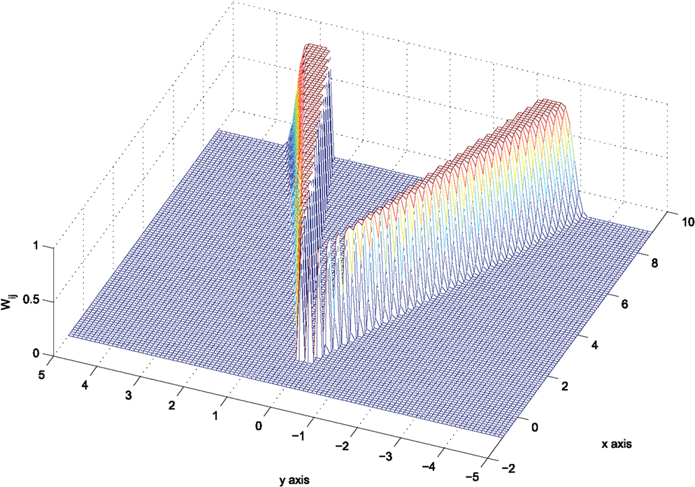
Figure 5. The function $W_{\mathit{ij}}=1-e^{-w_{\mathit{ij}}}$, given by equation (19).

In order to combine equations (13) and (19) into a single function that varies between zero and one, define:

$P_{\mathit{ij}}=V_{\mathit{ij}}{W}_{\mathit{ij}},$ (20)

which vanishes when at least one of the functions in equation (13), equation (19) vanishes, and varies in (0,1) anywhere else. However, this function does not penalize system trajectories with |ϕ_ij(t) < β| from tending to ||p_ij|| = r, or in simpler words, it does not encode that agent i maintains a safe distance ||p_ij|| > r (w.r.t) agent j when |ϕ_ij(t) < β|. For this reason, we consider the function:

${\mathrm{\sigma }}_{\mathit{ij}}=\left\{\begin{array}{cc}0,\hfill & \mathrm{if}\left|{\mathrm{\varphi }}_{\mathit{ij}}\right|<\mathrm{\beta }\hfill \\ \frac{\left|{\mathrm{\varphi }}_{\mathit{ij}}\right|-\mathrm{\beta }}{\mathrm{\alpha }-\mathrm{\beta }},\hfill & \mathrm{if}\mathrm{\beta }\le \left|{\mathrm{\varphi }}_{\mathit{ij}}\right|\le \mathrm{\alpha }\hfill \\ 1,\hfill & \mathrm{if}\left|{\mathrm{\varphi }}_{\mathit{ij}}\right|>\mathrm{\alpha }\hfill \end{array}\right.$ (21)

and encode the transition between the functions P_ij, V_ij as:

$A_{\mathit{ij}}={\mathrm{\sigma }}_{\mathit{ij}}{P}_{\mathit{ij}}+\left(1-{\mathrm{\sigma }}_{\mathit{ij}}\right)V_{\mathit{ij}}.$ (22)

This function now encodes that for |ϕ_ij| < β one has σ_ij = 0 and as thus A_ij = V_ij. This further reads that the term equation (13) is active in this region of the state space, rendering the desirable avoidance objective. The function equation (22) is depicted in Figure 6 for agent i positioned at p_i = [0 0]^T with θ_i = 0.

FIGURE 6

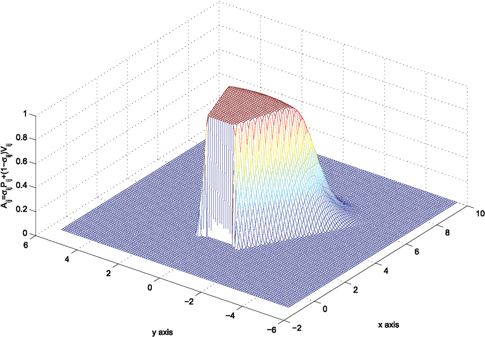
Figure 6. The avoidance function A_ij given by equation (22).

The bump function equation (21) defines three regions in the state space of agent i, in which the expression of equation (22) reads:

$A_{\mathit{ij}}=\left\{\begin{array}{cc}0,\hfill & \mathrm{if}{\mathrm{\sigma }}_{\mathit{ij}}=1\left(\mathrm{in}{R}_1\right)\hfill \\ {\mathrm{\sigma }}_{\mathit{ij}}{P}_{\mathit{ij}}+\left(1-{\mathrm{\sigma }}_{\mathit{ij}}\right)V_{\mathit{ij}},\hfill & \mathrm{if}0\le {\mathrm{\sigma }}_{\mathit{ij}}\le 1\left(\mathrm{in}{R}_2\right)\hfill \\ V_{\mathit{ij}},\hfill & \mathrm{if}{\mathrm{\sigma }}_{\mathit{ij}}=0\left(\mathrm{in}{R}_3\right).\hfill \end{array}\right.$ (23)

It can be easily verified after some algebraic calculations that: $\frac{\partial {\mathrm{\sigma }}_{\mathit{ij}}}{\partial p_i}=-\frac{\partial {\mathrm{\sigma }}_{\mathit{ij}}}{\partial p_j}$. Then, making use of equations (15) and (18), it is straightforward to verify that the following symmetry relation between the gradient vectors of A_ij (w.r.t), the position vectors p_i and p_j holds everywhere:

$\frac{\partial A_{\mathit{ij}}}{\partial p_i}=-\frac{\partial A_{\mathit{ij}}}{\partial p_j}.$ (24)

Of course, the analytical expressions of ∂A_ij/∂p_i in each of the three regions of the state space of agent i do not coincide, as it will furthermore become evident in the next section.

Finally, note that the construction of a conical avoidance function for agent i (w.r.t) an agent j lying in the backward sensing footprint ${\mathcal{S}}_i^{\prime }$ follows exactly the same logic, with the difference that the angle ϕ_ij takes values in the interval [π + θ_i − α, π + θ_i + α], instead of the interval [θ_i − α, θ_i + α], and is omitted here in the interest of space.

2.3.3. Control strategy for pairwise collision avoidance

The function A_ij given by equation (23) serves as an encoding of collision avoidance for agent i (w.r.t) agent j. Studying the evolution of its time derivative (w.r.t), the system trajectories may thus offer a way of designing control strategies that realize the safety of the overall multi-agent system. The time derivative of equation (23) reads:

$\frac{d{A}_{\mathit{ij}}}{\mathit{dt}}=\frac{\partial A_{\mathit{ij}}}{\partial p_i}\left(\frac{d{p}_i}{\mathit{dt}}-\frac{d{p}_j}{\mathit{dt}}\right)+\frac{\partial A_{\mathit{ij}}}{\partial {\mathrm{\theta }}_i}{\mathrm{\omega }}_i+\frac{\partial A_{\mathit{ij}}}{\partial {\mathrm{\theta }}_j}{\mathrm{\omega }}_j,$ (25)

where $\frac{\partial A_{\mathit{ij}}}{\partial q_k}=\left[\begin{array}{ccc}\hfill \frac{\partial A_{\mathit{ij}}}{\partial x_k}\hfill & \hfill \frac{\partial A_{\mathit{ij}}}{\partial y_k}\hfill & \hfill \frac{\partial A_{\mathit{ij}}}{\partial {\mathrm{\theta }}_k}\hfill \end{array}\right]$, k ∈ {i, j}.

Theorem 2. Assuming pairwise interactions among agents, collisions are avoided under the control strategy:

$\left(u_i,{\mathrm{\omega }}_i\right)=\left\{\begin{array}{cc}\left(u_i^{\mathit{cov}},{\mathrm{\omega }}_i^{\mathit{cov}}\right),\hfill & \mathrm{if}{\mathrm{\sigma }}_{\mathit{ij}}=1\hfill \\ \left(u_i^{\mathit{av}},{\mathrm{\omega }}_i^{\mathit{av}}\right),\hfill & \mathrm{if}0<{\mathrm{\sigma }}_{\mathit{ij}}<1\hfill \\ \left(u_i^{\mathit{av}},{\mathrm{\omega }}_i^{\mathit{cov}}\right),\hfill & \mathrm{if}{\mathrm{\sigma }}_{\mathit{ij}}=0\hfill \end{array}\right.$ (26)

where $\left(u_i^{\mathit{cov}},{\mathrm{\omega }}_i^{\mathit{cov}}\right)$ is given by equation (11) and

$\begin{array}{ll}\hfill u_i^{\mathit{av}}& =-k_i,\mathrm{where}{k}_i>\frac{3k_u^{\mathit{cov}}\mathrm{\alpha }{\left(C^{\star }R\right)}^2}{\cos \mathrm{\alpha }},\end{array}$ (27a)

$\begin{array}{ll}\hfill {\mathrm{\omega }}_i^{\mathit{av}}& =-\frac{1}{{∥p_{\mathit{ij}}∥}^2}\left[\begin{array}{cc}{y}_{\mathit{ij}}& -x_{\mathit{ij}}\end{array}\right]\left(\frac{d{p}_i}{\mathit{dt}}-\frac{d{p}_j}{\mathit{dt}}\right).\end{array}$ (27b)

Proof. Let us study the evolution of the time derivative of equation (23) in each region of the state space.

$\begin{array}{ll}\hfill \frac{\partial A_{\mathit{ij}}}{\partial p_i}& ={\mathrm{\sigma }}_{\mathit{ij}}\frac{\partial \left(V_{\mathit{ij}}{W}_{\mathit{ij}}\right)}{\partial p_i}+\frac{\partial {\mathrm{\sigma }}_{\mathit{ij}}}{\partial p_i}\left(V_{\mathit{ij}}{W}_{\mathit{ij}}\right)+\left(1-{\mathrm{\sigma }}_{\mathit{ij}}\right)\frac{\partial V_{\mathit{ij}}}{\partial p_i}-\frac{\partial a_{\mathit{ij}}}{\partial p_i}{V}_{\mathit{ij}}\\ \hfill & ={\mathrm{\sigma }}_{\mathit{ij}}\left(W_{\mathit{ij}}\frac{\partial V_{\mathit{ij}}}{\partial p_i}+V_{\mathit{ij}}\frac{\partial W_{\mathit{ij}}}{\partial p_i}\right)+\frac{\partial {\mathrm{\sigma }}_{\mathit{ij}}}{\partial p_i}\left(V_{\mathit{ij}}{W}_{\mathit{ij}}\right)+\left(1-{\mathrm{\sigma }}_{\mathit{ij}}\right)\frac{\partial V_{\mathit{ij}}}{\partial p_i}-\frac{\partial {\mathrm{\sigma }}_{\mathit{ij}}}{\partial p_i}{V}_{\mathit{ij}}\\ \hfill & ={\mathrm{\sigma }}_{\mathit{ij}}\left(W_{\mathit{ij}}{e}^{-v_{\mathit{ij}}}\frac{\partial v_{\mathit{ij}}}{\partial p_i}+V_{\mathit{ij}}{e}^{-w_{\mathit{ij}}}\frac{\partial w_{\mathit{ij}}}{\partial p_i}\right)+\frac{\partial {\mathrm{\sigma }}_{\mathit{ij}}}{\partial p_i}{V}_{\mathit{ij}}\left(W_{\mathit{ij}}-1\right)+\left(1-{\mathrm{\sigma }}_{\mathit{ij}}\right)e^{-v_{\mathit{ij}}}\frac{\partial v_{\mathit{ij}}}{\partial p_i}\\ \hfill & ={\mathrm{\sigma }}_{\mathit{ij}}\left(W_{\mathit{ij}}{e}^{-v_{\mathit{ij}}}\frac{\partial v_{\mathit{ij}}}{\partial p_i}+V_{\mathit{ij}}{e}^{-w_{\mathit{ij}}}\frac{\partial w_{\mathit{ij}}}{\partial p_i}\right)-\frac{1}{\left(\mathrm{\alpha }-\mathrm{\beta }\right){\mathrm{\Psi }}_{\mathit{ij}}}\frac{\partial w_{\mathit{ij}}}{\partial p_i}{V}_{\mathit{ij}}\left(W_{\mathit{ij}}-1\right)+\left(1-{\mathrm{\sigma }}_{\mathit{ij}}\right)e^{-v_{\mathit{ij}}}\frac{\partial v_{\mathit{ij}}}{\partial p_i}\\ \hfill & =\frac{\partial v_{\mathit{ij}}}{\partial p_i}{e}^{-v_{\mathit{ij}}}\left(1+{\mathrm{\sigma }}_{\mathit{ij}}\left(W_{\mathit{ij}}-1\right)\right)+\frac{\partial w_{\mathit{ij}}}{\partial p_i}{V}_{\mathit{ij}}\left({\mathrm{\sigma }}_{\mathit{ij}}{e}^{-w_{\mathit{ij}}}-\frac{1}{\left(\mathrm{\alpha }-\mathrm{\beta }\right){\mathrm{\Psi }}_{\mathit{ij}}}\left(W_{\mathit{ij}}-1\right)\right)\\ \hfill & =\frac{\partial v_{\mathit{ij}}}{\partial p_i}{e}^{-v_{\mathit{ij}}}\left(1-{\mathrm{\sigma }}_{\mathit{ij}}{e}^{-w_{\mathit{ij}}}\right)+\frac{\partial w_{\mathit{ij}}}{\partial p_i}{V}_{\mathit{ij}}\left({\mathrm{\sigma }}_{\mathit{ij}}{e}^{-w_{\mathit{ij}}}+\frac{1}{\left(\mathrm{\alpha }-\mathrm{\beta }\right){\mathrm{\Psi }}_{\mathit{ij}}}{e}^{-w_{\mathit{ij}}}\right)\\ \hfill & =\frac{\partial v_{\mathit{ij}}}{\partial p_i}{e}^{-v_{\mathit{ij}}}\left(1-{\mathrm{\sigma }}_{\mathit{ij}}{e}^{-w_{\mathit{ij}}}\right)+\frac{\partial w_{\mathit{ij}}}{\partial p_i}\left(1-e^{-v_{\mathit{ij}}}\right)e^{-w_{\mathit{ij}}}\left({\mathrm{\sigma }}_{\mathit{ij}}+\frac{1}{\left(\mathrm{\alpha }-\mathrm{\beta }\right){\mathrm{\Psi }}_{\mathit{ij}}}\right),\end{array}$ (28a)

$\begin{array}{llll}\hfill \frac{\partial A_{\mathit{ij}}}{\partial {\mathrm{\theta }}_i}& ={\mathrm{\sigma }}_{\mathit{ij}}\left(W_{\mathit{ij}}\frac{\partial V_{\mathit{ij}}}{\partial {\mathrm{\theta }}_i}+V_{\mathit{ij}}\frac{\partial W_{\mathit{ij}}}{\partial {\mathrm{\theta }}_i}\right)+\frac{\partial {\mathrm{\sigma }}_{\mathit{ij}}}{\partial {\mathrm{\theta }}_i}\left(V_{\mathit{ij}}{W}_{\mathit{ij}}\right)+\left(1-{\mathrm{\sigma }}_{\mathit{ij}}\right)\frac{\partial V_{\mathit{ij}}}{\partial {\mathrm{\theta }}_i}-\frac{\partial {\mathrm{\sigma }}_{\mathit{ij}}}{\partial {\mathrm{\theta }}_i}{V}_{\mathit{ij}}& \hfill & \\ \hfill & ={\mathrm{\sigma }}_{\mathit{ij}}{V}_{\mathit{ij}}{e}^{-w_{\mathit{ij}}}\frac{\partial w_{\mathit{ij}}}{\partial {\mathrm{\theta }}_i}+\frac{\partial {\mathrm{\sigma }}_{\mathit{ij}}}{\partial {\mathrm{\theta }}_i}{V}_{\mathit{ij}}\left(W_{\mathit{ij}}-1\right)& \hfill & \\ \hfill & ={\mathrm{\sigma }}_{\mathit{ij}}{V}_{\mathit{ij}}{e}^{-w_{\mathit{ij}}}\frac{\partial w_{\mathit{ij}}}{\partial {\mathrm{\theta }}_i}-\frac{\partial {\mathrm{\sigma }}_{\mathit{ij}}}{\partial {\mathrm{\theta }}_i}{V}_{\mathit{ij}}{e}^{-w_{\mathit{ij}}}=V_{\mathit{ij}}{e}^{-w_{\mathit{ij}}}\left({\mathrm{\sigma }}_{\mathit{ij}}\frac{\partial w_{\mathit{ij}}}{\partial {\mathrm{\theta }}_i}-\frac{\partial {\mathrm{\sigma }}_{\mathit{ij}}}{\partial {\mathrm{\theta }}_i}\right)& \hfill & \\ \hfill & ={\mathrm{\Psi }}_{\mathit{ij}}\left(1-e^{-v_{\mathit{ij}}}\right)e^{-w_{\mathit{ij}}}\left({\mathrm{\sigma }}_{\mathit{ij}}+\frac{1}{\left(\mathrm{\alpha }-\mathrm{\beta }\right){\mathrm{\Psi }}_{\mathit{ij}}}\right),\end{array}$ (28b)

$\begin{array}{ll}\hfill \frac{\partial A_{\mathit{ij}}}{\partial {\mathrm{\theta }}_j}& =0.\end{array}$ (28c)

2.3.4. Region R₁

In this region, one has: σ_ij = 1 ⇔ |ϕ_ij| ≥ α. Then, out of equation (23): A_ij = 0. This implies that agent i does not take into account the collision avoidance objective for any agent j ≠ i which lies out of the sensing area ${\mathcal{S}}_i$. The linear and angular velocity for agent i may thus be dictated by the coverage control law equation (11).

2.3.5. Region R₂

In this region, one has: 0 < σ_ij < 1 ⇔ β < |ϕ_ij| < α. Then out of equation (23): $A_{\mathit{ij}}={\mathrm{\sigma }}_{\mathit{ij}}{P}_{\mathit{ij}}+\left(1-{\mathrm{\sigma }}_{\mathit{ij}}\right)V_{\mathit{ij}}$.

The analytical expression of the gradients involved in equation (25) in this case is given by equation (28), where:

$\begin{array}{ll}\hfill \frac{\partial {\mathrm{\sigma }}_{\mathit{ij}}}{\partial p_i}& =-\frac{1}{\left(\mathrm{\alpha }-\mathrm{\beta }\right){\mathrm{\Psi }}_{\mathit{ij}}}\frac{\partial w_{\mathit{ij}}}{\partial p_i},\end{array}$ (29a)

$\begin{array}{ll}\hfill \frac{\partial {\mathrm{\sigma }}_{\mathit{ij}}}{\partial {\mathrm{\theta }}_i}& =-\frac{1}{\left(\mathrm{\alpha }-\mathrm{\beta }\right){\mathrm{\Psi }}_{\mathit{ij}}}\frac{\partial w_{\mathit{ij}}}{\partial {\mathrm{\theta }}_i}=-\frac{1}{\mathrm{\alpha }-\mathrm{\beta }}.\end{array}$ (29b)

Plugging equation (28) into equation (25) yields equation (30):

$\begin{array}{ll}\hfill \frac{d{A}_{\mathit{ij}}}{\mathit{dt}}& =\left(e^{-v_{\mathit{ij}}}\left(1-{\mathrm{\sigma }}_{\mathit{ij}}{e}^{-w_{\mathit{ij}}}\right)\frac{\partial v_{\mathit{ij}}}{\partial p_i}+e^{-w_{\mathit{ij}}}\left(1-e^{-v_{\mathit{ij}}}\right)\right.\left.\times \left({\mathrm{\sigma }}_{\mathit{ij}}+\frac{1}{\left(\mathrm{\alpha }-\mathrm{\beta }\right){\mathrm{\Psi }}_{\mathit{ij}}}\right)\frac{\partial w_{\mathit{ij}}}{\partial p_i}\right)\left(\frac{d{p}_i}{\mathit{dt}}-\frac{d{p}_j}{\mathit{dt}}\right)\\ \hfill & +{\mathrm{\Psi }}_{\mathit{ij}}{e}^{-w_{\mathit{ij}}}\left(1-e^{-v_{\mathit{ij}}}\right)\left({\mathrm{\sigma }}_{\mathit{ij}}+\frac{1}{\left(\mathrm{\alpha }-\mathrm{\beta }\right){\mathrm{\Psi }}_{\mathit{ij}}}\right){\mathrm{\omega }}_i\\ \hfill & =e^{-v_{\mathit{ij}}}\left(1-{\mathrm{\sigma }}_{\mathit{ij}}{e}^{-w_{\mathit{ij}}}\right)\frac{\partial v_{\mathit{ij}}}{\partial p_i}\left(\frac{d{p}_i}{\mathit{dt}}-\frac{d{p}_j}{\mathit{dt}}\right)+{\mathrm{\Psi }}_{\mathit{ij}}{e}^{-w_{\mathit{ij}}}\left(1-e^{-v_{\mathit{ij}}}\right)\left({\mathrm{\sigma }}_{\mathit{ij}}+\frac{1}{\left(\mathrm{\alpha }-\mathrm{\beta }\right){\mathrm{\Psi }}_{\mathit{ij}}}\right){\mathrm{\omega }}_i\\ \hfill & +\left(e^{-w_{\mathit{ij}}}\left(1-e^{-v_{\mathit{ij}}}\right)\left({\mathrm{\sigma }}_{\mathit{ij}}+\frac{1}{\left(\mathrm{\alpha }-\mathrm{\beta }\right){\mathrm{\Psi }}_{\mathit{ij}}}\right)\right.\left.\times \frac{{\mathrm{\Psi }}_{\mathit{ij}}}{{∥p_{\mathit{ij}}∥}^2}\left[\begin{array}{cc}\hfill y_{\mathit{ij}}\hfill & \hfill -x_{\mathit{ij}}\hfill \end{array}\right]\right)\left(\frac{d{p}_i}{\mathit{dt}}-\frac{d{p}_j}{\mathit{dt}}\right),\end{array}$ (30)

while substituting the angular velocity equation (27b) of agent i into equation (30) yields:

$\begin{array}{llll}\hfill \frac{d{A}_{\mathit{ij}}}{\mathit{dt}}& =e^{-v_{\mathit{ij}}}\left(1-{\mathrm{\sigma }}_{\mathit{ij}}{e}^{-w_{\mathit{ij}}}\right)\frac{\partial v_{\mathit{ij}}}{\partial p_i}\left(\frac{d{p}_i}{\mathit{dt}}-\frac{d{p}_j}{\mathit{dt}}\right)& \hfill & \\ \hfill & (14)\\ \hfill & =e^{-v_{ij}}\left(1-{\mathrm{\sigma }}_{\mathit{ij}}{e}^{-w_{\mathit{ij}}}\right){\mathrm{\Omega }}_{ij}& \hfill & \\ \hfill & =-e^{-v_{\mathit{ij}}}\left(1-{\mathrm{\sigma }}_{\mathit{ij}}{e}^{-w_{\mathit{ij}}}\right)\left|{\mathrm{\Omega }}_{\mathit{ij}}\right|\times \left(p_{\mathit{ij}}{}^T\left[\begin{array}{c}\cos {\theta }_i\\ \sin {\theta }_i\end{array}\right]u_i-{p_{\mathit{ij}}}^T\left[\begin{array}{c}\cos {\theta }_j\\ \sin {\theta }_j\end{array}\right]u_j\right)& \hfill & \\ \hfill & =-e^{-v_{\mathit{ij}}}\left(1-{\mathrm{\sigma }}_{\mathit{ij}}{e}^{-w_{\mathit{ij}}}\right)\left|{\mathrm{\Omega }}_{\mathit{ij}}\right|\times \left(p_{ij}{}^T\left[\begin{array}{c}\cos {\theta }_i\\ \sin {\theta }_i\end{array}\right]u+p_{ij}{}^T\left[\begin{array}{c}\cos {\theta }_j\\ \sin {\theta }_j\end{array}\right]u_j\right),& \hfill & \end{array}$

so that one finally has:

$\frac{d{A}_{\mathit{ij}}}{\mathit{dt}}=-e^{-v_{\mathit{ij}}}\left(1-{\mathrm{\sigma }}_{\mathit{ij}}{e}^{-w_{\mathit{ij}}}\right)\left|{\mathrm{\Omega }}_{\mathit{ij}}\right|{p_{\mathit{ij}}}^T\left[\begin{array}{c}\cos {\theta }_i\\ \sin {\theta }_i\end{array}\right]u_i-e^{-v_{\mathit{ij}}}\left(1-{\mathrm{\sigma }}_{\mathit{ij}}{e}^{-w_{\mathit{ij}}}\right)\left|{\mathrm{\Omega }}_{\mathit{ij}}\right|{p_{\mathit{ji}}}^T\left[\begin{array}{c}\cos {\theta }_j\\ \sin {\theta }_j\end{array}\right]u_j,$ (31)

where p_ij = p_i − p_j, p_ji = p_j − p_i and Ω_ij < 0.

In region R₂, it always holds that: $p_{\mathit{ij}}{}^T\left[\begin{array}{c}\cos {\theta }_i\\ \sin {\theta }_i\end{array}\right]<0$. Thus, if the linear velocity u_i of agent i is set as u_i < 0, then the first term of the time derivative equation (31) is negative.

Consider the velocity equation (27a) where k_i > 0, and study the effect of the second term in the evolution of the time derivative equation (31). Clearly, this depends on the orientation θ_j of agent j and its linear velocity u_j. Let us consider the following cases.

2.3.5.1. Agent i lies in the sensing area ${\mathcal{S}}_j$ of agent j. Then, for the same reasoning as for agent i, agent j realizes its own Lyapunov-like avoidance function A_ji, given by equation (22) after replacing i with j and vice versa. The time derivative of this function, after setting the angular velocity w_j equal to:

${\mathrm{\omega }}_j{}^{av}=-\frac{1}{{∥p_{\mathit{ji}}∥}^2}\left[\begin{array}{cc}\hfill y_{\mathit{ji}}\hfill & \hfill -x_{\mathit{ji}}\hfill \end{array}\right]\left(\frac{d{p}_j}{\mathit{dt}}-\frac{d{p}_i}{\mathit{dt}}\right),$ (32)

ends up reading:

$\frac{d{A}_{\mathit{ji}}}{\mathit{dt}}=-e^{-v_{\mathit{ji}}}\left(1-{\mathrm{\sigma }}_{\mathit{ji}}{e}^{-w_{\mathit{ji}}}\right)\left|{\mathrm{\Omega }}_{\mathit{ji}}\right|{p_{\mathit{ji}}}^T\left[\begin{array}{c}\cos {\theta }_j\\ \sin {\theta }_j\end{array}\right]u_j+k_i{e}^{-v_{\mathit{ji}}}\left(1-{\mathrm{\sigma }}_{\mathit{ji}}{e}^{-w_{\mathit{ji}}}\right)\left|{\mathrm{\Omega }}_{\mathit{ji}}\right|{p_{\mathit{ij}}}^T\left[\begin{array}{c}\cos {\theta }_i\\ \sin {\theta }_i\end{array}\right],$ (33)

where $p_{ji}{}^T\left[\begin{array}{c}\cos {\mathrm{\theta }}_j\\ \sin {\mathrm{\theta }}_j\end{array}\right]<0$ and the second term in equation (33) is non-positive.

Then setting the linear velocity for agent j equal to:

${u_j}^{\mathit{av}}=-k_j,$ (34)

renders the first term in equation (33) negative. Note that the angular velocities equations (27b) and (32) coincide, which is consistent with what one would expect from physical intuition; namely, that for agents i and j facing each other, it is plausible to both rotate either clockwise, or counterclockwise, to avoid collision.

2.3.5.2. Agent i does not lie in the sensing area ${\mathcal{S}}_j$ of agent j. This implies that agent j moves under the coverage control law $u_j^{\mathit{cov}}$. The signum of the linear velocity $u_j^{\mathit{cov}}$ depends on the signum of $\left({\frac{\partial S_j}{\partial p_j}}^T\left[\begin{array}{c}\cos {\mathrm{\theta }}_j\\ \sin {\mathrm{\theta }}_j\end{array}\right]\right)$. Also, one has that:

$\begin{array}{lll}\hfill \left|u_j^{\mathit{cov}}\right|\le k_u^{\mathit{cov}}3{\left(C^{\star }\right)}^2\left(\mathrm{\alpha }{R}^2\right).& & \hfill \end{array}$

Let us go back to equation (31), which now reads:

$\begin{array}{lll}\hfill \frac{d{A}_{\mathit{ij}}}{\mathit{dt}}=-e^{-v_{\mathit{ij}}}\left(1-{\mathrm{\sigma }}_{\mathit{ij}}{e}^{-w_{\mathit{ij}}}\right)\left|{\mathrm{\Omega }}_{\mathit{ij}}\right|\times \left(\left|{p_{\mathit{ij}}}^T\left[\begin{array}{c}\cos {\theta }_i\\ \sin {\theta }_i\end{array}\right]\right|k_i+{p_{\mathit{ji}}}^T\left[\begin{array}{c}\cos {\theta }_j\\ \sin {\theta }_j\end{array}\right]u_j^{\mathit{cov}}\right),& & \hfill \end{array}$

and consider the following cases:

(a) $u_j^{\mathit{cov}}>0\frac{1}{2}$ and $p_{ji}{}^T\left[\begin{array}{c}\cos {\mathrm{\theta }}_j\\ \sin {\mathrm{\theta }}_j\end{array}\right]\ge 0$ : then $\frac{d{A}_{\mathit{ij}}}{\mathit{dt}}\le 0$, ensuring that collision is avoided.

(b) $u_j^{\mathit{cov}}>0$ and $p_{ji}{}^T\left[\begin{array}{c}\cos {\mathrm{\theta }}_j\\ \sin {\mathrm{\theta }}_j\end{array}\right]<0$ : then a sufficient condition on avoiding collision is to set:

$\left|{p_{\mathit{ij}}}^T\left[\begin{array}{c}\hfill \cos {\mathrm{\theta }}_i\hfill \\ \hfill \sin {\mathrm{\theta }}_i\hfill \end{array}\right]\right|k_i>\left|{p_{\mathit{ji}}}^T\left[\begin{array}{c}\hfill \cos {\mathrm{\theta }}_j\hfill \\ \hfill \sin {\mathrm{\theta }}_j\hfill \end{array}\right]\right|u_j^{\mathit{cov}}.$

Now note that:

$\left|{p_{\mathit{ji}}}^T\left[\begin{array}{c}\hfill \cos {\mathrm{\theta }}_j\hfill \\ \hfill \sin {\mathrm{\theta }}_j\hfill \end{array}\right]\right|u_j^{\mathit{cov}}\le ∥p_{\mathit{ji}}∥3k_u^{\mathit{cov}}\mathrm{\alpha }{\left(C^{\star }R\right)}^2,$

which further reads that it suffices to choose the control gains $k_i,k_u^{\mathit{cov}}$ so that:

$\left|{p_{\mathit{ij}}}^T\left[\begin{array}{c}\hfill \cos {\mathrm{\theta }}_i\hfill \\ \hfill \sin {\mathrm{\theta }}_i\hfill \end{array}\right]\right|k_i>∥p_{\mathit{ji}}∥3k_u^{\mathit{cov}}\mathrm{\alpha }{\left(C^{\star }R\right)}^2.$

Furthermore, in this region of the state space one has that: $\underset{p_j\in S_i}{\min }\left(|p_{ji}{}^T\left[\begin{array}{c}\cos {\mathrm{\theta }}_i\\ \sin {\mathrm{\theta }}_i\end{array}\right]\right)=r\cos \mathrm{\alpha }$.¹ Consequently, it suffices to pick the avoidance control gain:

$k_i>\frac{3k_u^{\mathit{cov}}\mathrm{\alpha }{\left(C^{\star }R\right)}^2}{\cos \mathrm{\alpha }}.$ (35)

(c)  $u_j^{\mathit{cov}}<0$ and $p_{ji}{}^T\left[\begin{array}{c}\cos {\mathrm{\theta }}_j\\ \sin {\mathrm{\theta }}_j\end{array}\right]\ge 0$ : same as case (b).

(d) $u_j^{\mathit{cov}}<0$ and $p_{ji}{}^T\left[\begin{array}{c}\cos {\mathrm{\theta }}_j\\ \sin {\mathrm{\theta }}_j\end{array}\right]<0$ : same as case (a).

2.3.6. Region R₃

In this region, one has: σ_ij = 0 ⇔ |ϕ_ij| ≤ β. Then out of equation (22): A_ij = V_ij. Then:

$\frac{d{A}_{\mathit{ij}}}{\mathit{dt}}=-e^{-v_{\mathit{ij}}}\left|{\mathrm{\Omega }}_{\mathit{ij}}\right|\left({p_{\mathit{ij}}}^T\left[\begin{array}{c}\hfill \cos {\mathrm{\theta }}_i\hfill \\ \hfill \sin {\mathrm{\theta }}_i\hfill \end{array}\right]u_i+{p_{\mathit{ji}}}^T\left[\begin{array}{c}\hfill \cos {\mathrm{\theta }}_j\hfill \\ \hfill \sin {\mathrm{\theta }}_j\hfill \end{array}\right]u_j\right).$

This case reduces to equation (31) after setting σ_ij = 0; thus, the same analysis as in the previous case follows regarding the linear velocity u_i, which is set equal to $u_i^{\mathit{av}}$ equation (27a). The angular velocity ω_i is set equal to ${\mathrm{\omega }}_i^{\mathit{cov}}$.

The angular velocity control law equation (27b) for agent i requires information involving the state and control vectors of agent j, through the effect of dp_j/dt. Denote $p_{\mathit{ij}}^{\star }={\left[\begin{array}{cc}\hfill y_{\mathit{ij}}\hfill & \hfill -x_{\mathit{ij}}\hfill \end{array}\right]}^T$ the orthogonal vector to p_ij and consider the analytical expression of equation (27b), which reads:

${\mathrm{\omega }}_i^{\mathit{av}}=-\frac{\left|{p_{\mathit{ij}}^{\star }}^T\left[\begin{array}{c}\hfill \cos {\mathrm{\theta }}_i\hfill \\ \hfill \sin {\mathrm{\theta }}_i\hfill \end{array}\right]\right|k_i}{{∥p_{\mathit{ij}}∥}^2}-\frac{{p_{\mathit{ji}}^{\star }}^T\left[\begin{array}{c}\hfill \cos {\mathrm{\theta }}_j\hfill \\ \hfill \sin {\mathrm{\theta }}_j\hfill \end{array}\right]u_j}{{∥p_{\mathit{ij}}∥}^2}.$ (36)

The first term of equation (36) depends on the state vector of agent i only, and dictates that agent i should rotate clockwise (recall that we are considering the case ϕ_ij > 0), forcing thus the sensing area ${\mathcal{S}}_i$ away from agent j.

Finally, we would like to explore conditions under which the resulting maneuvering is sufficient for ensuring collision avoidance but without the need for information exchange between agents i and j, i.e., under the assumption that agent i does not sense or measure the linear velocity u_j and the orientation θ_j of agent j and vice versa. This may also be seen as a robustness feature in the presence of communication failures.

To study the effect of the motion of agent j through u_j and θ_j in equation (36), we consider the following two cases:

2.3.6.1. Agent i lies in the sensing area ${\mathcal{S}}_j$ of agent j. Then, equation (36) further reads:

${\mathrm{\omega }}_i^{\mathit{av}}=-\frac{\left|{p_{\mathit{ij}}^{\star }}^T\left[\begin{array}{c}\hfill \cos {\mathrm{\theta }}_i\hfill \\ \hfill \sin {\mathrm{\theta }}_i\hfill \end{array}\right]\right|k_i}{{∥p_{\mathit{ij}}∥}^2}+\frac{{p_{\mathit{ji}}^{\star }}^T\left[\begin{array}{c}\hfill \cos {\mathrm{\theta }}_j\hfill \\ \hfill \sin {\mathrm{\theta }}_j\hfill \end{array}\right]k_j}{{∥p_{\mathit{ij}}∥}^2}.$ (37)

The signum of $p_{ji}^{\star T}\left[\begin{array}{c}\cos {\mathrm{\theta }}_j\\ \sin {\mathrm{\theta }}_j\end{array}\right]$ dictates the signum of the second term. More specifically:

(a) If $p_{ji}^{\star T}\left[\begin{array}{c}\cos {\mathrm{\theta }}_j\\ \sin {\mathrm{\theta }}_j\end{array}\right]<0\iff {\mathrm{\varphi }}_{\mathit{ji}}>0$ : the second term is then negative, and furthermore renders a clockwise rotation for agent j. This condition (i.e., both agents rotating along the same direction) has the effect of setting each one out of the sensing area of the other. Consequently, the angular velocity ${\mathrm{\omega }}_i^{\mathit{av}}$ for agent i can be taken out of equation (27b) with dp_j/dt = 0.

(b) If $p_{ji}^{\star T}\left[\begin{array}{c}\cos {\mathrm{\theta }}_j\\ \sin {\mathrm{\theta }}_j\end{array}\right]>0\iff {\mathrm{\varphi }}_{\mathit{ji}}<0$ : the second term is then positive, and furthermore renders a counterclockwise rotation for agent j. We would like to make sure that the angular velocity ${\mathrm{\omega }}_i^{\mathit{av}}$ remains negative, i.e., that agent i will keep rotating clockwise to set agent j out of the sensing area ${\mathcal{S}}_i$. This condition reads:

$k_j\underset{p_i\in S_j}{\max }\left({p_{\mathit{ji}}^{\star }}^T\left[\begin{array}{c}\hfill \cos {\mathrm{\theta }}_j\hfill \\ \hfill \sin {\mathrm{\theta }}_j\hfill \end{array}\right]\right)<k_i\underset{p_j\in S_i}{\min }\left(\left|{p_{\mathit{ij}}^{\star }}^T\left[\begin{array}{c}\hfill \cos {\mathrm{\theta }}_i\hfill \\ \hfill \sin {\mathrm{\beta }}_i\hfill \end{array}\right]\right|\right).$ (38)

It is now easy to verify that: (i) The maximum value of $p_{ji}^{\star T}\left[\begin{array}{c}\cos {\theta }_i\\ \sin {\theta }_i\end{array}\right]$ is achieved for agent i lying on the boundary of ${\mathcal{S}}_j$, where ϕ_ji = −α. Thus, $\underset{p_i\in S_j}{\max }\left(p_{ji}^{\star T}\left[\begin{array}{c}\cos {\theta }_j\\ \sin \theta j\end{array}\right]\right)=\left|\right|p_{\mathit{ij}}\left|\right|\sin \mathrm{\alpha }$. (ii) The minimum value of $\left|p_{ij}^{\star T}\left[\begin{array}{c}\cos {\theta }_i\\ \sin {\theta }_i\end{array}\right]\right|$ is achieved for agent j lying on a point $p_j\mathrm{\in }{\mathcal{S}}_i$ such that ϕ_ij = β; recall that we are studying the case when β < ϕ_ij < α. Thus, $\underset{p_j\in S_i}{\min }\left(\left|p_{ij}^{\star T}\left[\begin{array}{c}\cos {\theta }_i\\ \sin {\theta }_i\end{array}\right]\right|\right)=\left|\right|p_{\mathit{ij}}\left|\right|\sin \mathrm{\beta }$.

Substituting these values in equation (38) further yields: k_j sin α < k_j sin β. It is noteworthy that for k_i = k_j this inequality does not hold since 0 < β < α < π/2. This further means that we can not get any guarantees on the signum of the angular velocity ${\mathrm{\omega }}_i^{\mathit{av}},$ unless we assume that the agents somehow exchange information on their control gains k_i, k_j (or their linear velocities u_i, u_j). Nevertheless, the condition equation (38) is quite conservative and only sufficient, not necessary. Furthermore, it does hold when the relative position of the agents i, j is such that: |ϕ_ji| < ϕ_ij. The condition for inter-agent collision avoidance is to ensure that ||p_ij|| > r, which is ensured through the linear control laws $u_i^{\mathit{av}},u_j^{\mathit{av}}$.

2.3.6.2. Agent i does not lie in the sensing area ${\mathcal{S}}_j$ of agent j. This further implies that agent j moves under the coverage control law $u_j^{\mathit{cov}}$. Then the problem reduces into guaranteeing that: $k_i>\left|u_j^{\mathit{cov}}\right|,$ which has been treated before.

3. Results

The proposed control strategy equation (26), equation (11), equation (27) is evaluated through numerical simulations. We consider a scenario of 5 agents with sensing capabilities realized as conical sensing functions, which need to sufficiently explore a relatively open area D populated with two circular static obstacles. The area is a rectangle of dimension d_a = 25, the obstacles are positioned at p_o1 = [11 15]^T, p_o2 = [15 5]^T, respectively, and are of radius r_o = 1. The satisfactory coverage level is set equal to C^⋆ = 0.7, and this selection is guided based on the maximum value of the considered sensing function S_i(⋅), which in this scenario is approximately 0.2. The sensing and coverage parameters are R = 6, r = 3, α = π/6. The agents know the positions and the geometry of the obstacles. The agents have also the ability of broadcast information to other agents regarding the areas they have individually covered, so that at least one agent (called the supervisor) has access to the globally covered area.

In Figures 7–9, dark blue stands for totally uncovered area (i.e., zero time has been spent on these points of D by the agents footprints), dark red stands for totally covered area (i.e., agents footprints have stayed on these points of D for the satisfactory amount of time encoded via C^⋆), while color variations between dark blue and dark red stand for partially covered area, i.e., for points of D, which have been sensed by the agents footprints but not for the satisfactory amount of time.

FIGURE 7

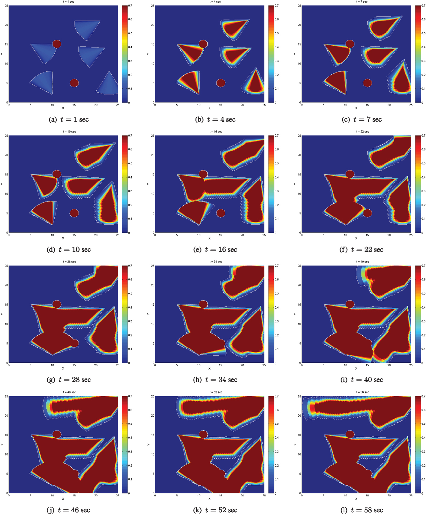
Figure 7. Evolution of the coverage level under the proposed control strategy equation (26).

FIGURE 8

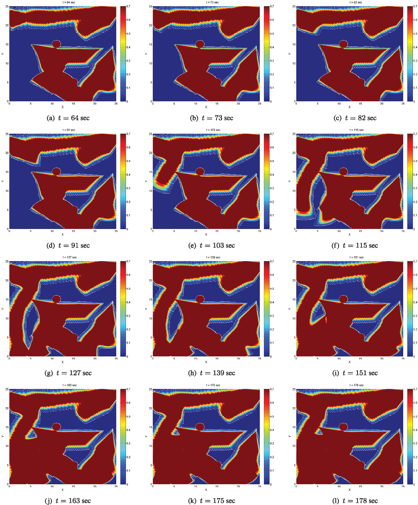
Figure 8. Evolution of the coverage level under the proposed control strategy equation (26).

FIGURE 9

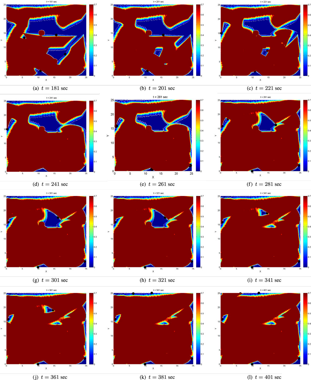
Figure 9. Evolution of the coverage level after the supervisory logic on global coverage has been activated for the first time.

The coverage level at initial time t = 0 is zero. Figures 7 and 8 depict the evolution of the coverage level over time under the control strategy equation (26) up to the time when all agents’ coverage errors equation (6) become very small, implying that the agents have practically stop moving. The boundaries of the sensing footprints are depicted with white lines. Focusing on the interior of the sensing footprints during at simulation time t = 1, one may notice that the color remains darker blue on the points closer to the boundaries of the footprints, while it gets lighter blue on the points closer to the centers of the footprints. This is consistent with the definition of the sensing function equation (4) and the coverage error equation (6) for each agent: recall that the sensing function equation (4) takes lower values close to the boundary of the sensing footprint, encoding that the sensor performance (“seeing”) is not good enough there, and higher values on the points in the interior and far away from the boundary, encoding that sensing performance is better there. Thus, more time is required to sense the points close to the boundary of the sensing footprint up to the satisfactory coverage level, and this is encoded via the coverage error equation (6). For this reason, the points in the interior of the sensing footprint but far away from its boundary turn red sooner than those closer to the boundary. Note also that the agents’ coverage errors equation (6) are exactly what sets them in motion via their coverage control laws equation (11). In other words, as long as the agents’ footprints touch points in D where the satisfactory coverage encoded via C^⋆ has not been met, their control inputs realized via equation (11) are non-zero and therefore the agents keep moving toward zeroing their coverage errors.

In general, the area of the satisfactorily covered regions by a given number of agents under the control law equation (11) depends on the coverage (sensing) function equation (4), the parameter C^⋆, the control law gains in equation (11), and the initial conditions. As expected and explained in Section 2.2, the agents may stop moving before the entire area D has necessarily been covered up to the satisfactory level. Let us define the global coverage error E(t) as the non-satisfactorily covered area at time t. In the considered scenario, the agents stop moving before the global coverage error E(t) has converged to zero; more specifically, the agents stop moving when almost 76% of the domain D has been sufficiently covered at time t = 180, as illustrated via the evolution of the (normalized) global coverage error E(t) in Figure 10A.

FIGURE 10

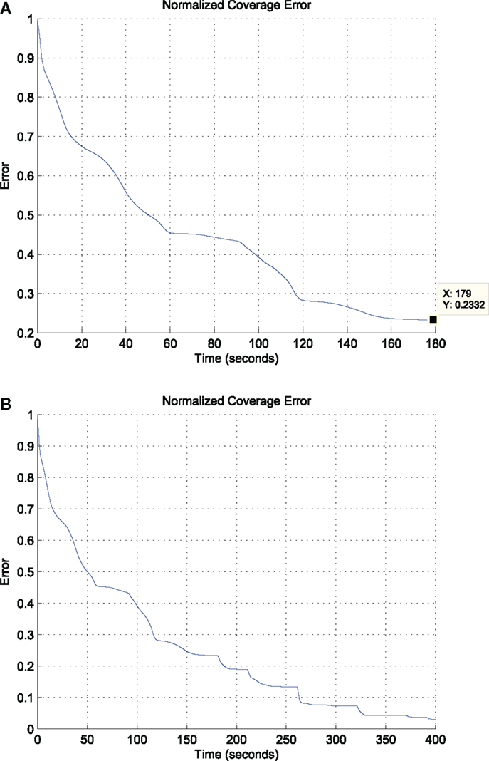
Figure 10. The evolution of the (normalized) global coverage error E(t) under (i) the proposed control strategy equation (26) (above) and (ii) under the same strategy facilitated with the supervisory global coverage controller, which takes action for the first time at time t = 180 (below). (A) Evolution of the global coverage error E(t) w.r.t time under the proposed control strategy equation (26). (B) Evolution of the global coverage error E(t) w.r.t time under the control strategy equation (26) and the supervisory logic on the global coverage control. The global coverage controller becomes active for the first time at time t = 180 and keeps getting active when the rate of change of the global coverage error E(t) becomes less than a given threshold.

A way to bypass this limitation is to additionally consider a global coverage controller, implemented by a supervisor agent who has an access to the coverage map of the environment, i.e., to the global coverage error E(t) at each time instant t, in the spirit proposed in Atinç et al. (2013). We modify the strategy in Atinç et al. (2013) to be compatible with the conic sensing footprints considered here. More specifically, we implement the following logic:

• If the normalized coverage error E(t_k) is non-zero at some time instant t_k and its absolute rate of change, realized as the difference |E(t_k) − E(t_k−1)/t_k − t_k−1| drops below a predefined level, then this physically means that the agents have driven their coverage errors e_i(t) very close to zero. Thus, the supervisor agent needs to select new waypoints within the uncovered areas toward which the agents will move.

• The selection of waypoints is performed under the (heuristic) formula suggested in Atinç et al. (2013), which provides the closest point in the uncovered region of the domain D for each one of the agents. This search for the closest uncovered point in principle returns points, which lie on the boundaries between covered and uncovered regions, see also Figure 9, the waypoints depicted as black circles.

• The motion of the agents toward their waypoints can be guaranteed to be safe under the algorithms in our prior work (Panagou et al., 2013); nevertheless, the motion of the agents toward their waypoints is not simulated here.

• Once an agent has reached its assigned waypoint, it performs an in place rotation so that its sensing footprint touches the uncovered area and its coverage error defined by equation (6) becomes non-zero. Note that this maneuvering was not necessary in Atinç et al. (2013), as the sensing footprints considered there are circular; however, it is essential when it comes to conic sensing footprints. The agent switches to its coverage control law equation (11) and starts moving toward driving its coverage error equation (6) to zero.

• This process, i.e., switching between local and global coverage controllers, is repeated as many times as necessary, so that the normalized coverage error E(t) is forced to decrease and eventually to converge to zero.

During the selection of waypoints, the supervisor agent makes sure that waypoints close to physical obstacles or points, which will result in agents approaching closer than the safe distance are excluded. Note also that the shape of the uncovered areas cannot be predicted a priori, as this would involve the computation of the forward reachable sets of all agents for any possible initial condition, something which is impossible due to the curse of dimensionality (or state explosion) even when only few agents are concerned. However, given the aforementioned constraints, it is not impossible that searching for the closest uncovered point may not provide a feasible solution. Thus, the supervisor additionally monitors whether this search produces new waypoints for the agents, otherwise it selects waypoints, which lie in the interior of the uncovered areas in a randomized way, i.e., does not pick the closest uncovered points. This is the case at time t = 263 s, where under this selection two of the agents are forced to move to waypoints lying in the interior, not the boundary, of the uncovered area. The evolution of the (normalized) global coverage error E(t) including the periods when the supervisory logic is active is depicted in Figure 10B. The error E(t) is decreasing, and the switching between global and local coverage controllers can be repeated as many times as necessary until it converges to zero.

The formalization of these set of rules within a suitable control theoretic framework, e.g., by means of switched systems theory, so that specific performance guarantees can be acquired for the supervisory controller is beyond the scope of the current paper. Addressing questions such as how an agent, or a group of agents, can select waypoints in the uncovered areas in more efficient ways, i.e., not merely selecting the closed uncovered point, but rather try to select points, which satisfy various objectives, such as minimizing the total number of switches between local and global coverage controllers is ongoing work.

The evolution of inter-agent distances and agent-static obstacle distances under the proposed control strategy equation (26), i.e., before the supervisory logic takes action for the first time, is depicted in Figure 11A. The effect of the collision avoiding maneuvers imposed when pertinent by equation (26) becomes evident through the trajectories, which end up in the detection regions of the agents’. The detection radius is illustrated in green, while the avoidance radius, which encodes the minimum safe distance, is illustrated in red. The distances remain always greater than the avoidance radius, implying that the motion of the agents remains collision-free. Again, it is important to stress out that this strategy is suitable for pairwise interactions only, and for this reason the number of the agents and their initial conditions are chosen such that agents are not congested. Finally, the resulting agents’ paths under equation (26) are illustrated in Figure 11B. Initial positions are depicted with dots, final positions are depicted with “x.” It is worth noticing that some agents tend to travel larger distances compared to others, compare for instance the blue path over the green path. The reason is that the agent in green starts close to the boundary of the domain D, and therefore as it starts rotating toward zeroing its coverage error, its sensing footprint ends up touching outside the domain D, where the coverage error is by definition zero.

FIGURE 11

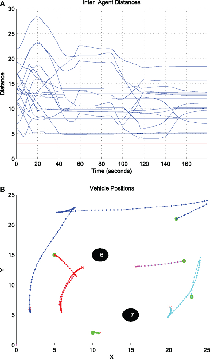
Figure 11. Inter-agent distances and resulting agents’ paths under the control strategy equation (26). (A) Evolution of the inter-agent distances d_ij w.r.t time under the control strategy equation (26). (B) The resulting paths under the control strategy equation (26).

4. Discussion

This paper presented a dynamic coverage control design for non-holonomic vehicles along with collision avoidance guarantees. The key difference compared to earlier similar work is the consideration of anisotropic sensing, which is relevant to vision-based control and surveillance applications. More specifically, we extended our earlier work (Panagou et al., 2013; Stipanovic et al., 2013) by considering a new dynamic coverage and avoidance control design, which can be implemented in a decentralizedfashion. The main difference here is the consideration of (i) anisotropic sensing, realized via conic sensing footprints and conic sensing (coverage) functions for each agent, and (ii) a novel form of avoidance functions. The considered sensing functions encode field-of-view and range constraints, and furthermore the degradation of effective sensing close to the boundaries of the sensing footprint. In this spirit, the proposed control design is suitable for surveillance tasks, where a group of robots is assigned with the task to gather enough information about an environment (such as video streaming or snapshots) locally, while avoiding collisions. The efficacy of the proposed control strategies has been demonstrated through numerical simulations for unicycle robots operating in a known environment populated with static circular obstacles.

Current work focuses on the consideration of supervisory logics to orchestrate efficient global coverage in a distributed sense along with certain performance guarantees, as well as on the consideration of agents with more complicated dynamics and constraints, such as Dubins-like vehicles.

Conflict of Interest Statement

The authors declare that the research was conducted in the absence of any commercial or financial relationships that could be construed as a potential conflict of interest.

Acknowledgments

This work has been supported by Qatar National Research Fund under NPRP Grant 4-536-2-199 and the AFOSR grant FA95501210193. The authors would like to acknowledge the contribution of Dr. G. Atinç and Dr. C. Valicka through fruitful discussions and their help on the simulation implementations.

Footnote

1. ^This inner product expresses the projection of the vector p_ij onto the $x_{B_i}$ body-fixed axis of agent i, while the value of this projection becomes minimum for agent j lying on the boundary of the sensing region of agent i, i.e., when ϕ_ij = α.

References

Atinç, G., Stipanovíc, D. M., Voulgaris, P. G., and Karkoub, M. (2013). “Supervised coverage control with guaranteed collision avoidance and proximity maintenance,” in Proc. of the 2013 IEEE Conference on Decision and Control (Florence), 3463–3468.

Google Scholar

Cheng, T. M., and Savkin, A. V. (2010). “Decentralized control of mobile sensor networks for triangular blanket coverage,” in Proc. of the 2010 American Control Conf (Baltimore, MD), 2903–2908.

Google Scholar

Corless, M., and Leitmann, G. (1989). Adaptive controllers for avoidance or evasion in an uncertain environment: some examples. Comput. Math. Appl. 18, 161–170. doi: 10.1016/0898-1221(89)90133-8

CrossRef Full Text | Google Scholar

Corless, M., Leitmann, G., and Skowronski, J. (1987). Adaptive control for avoidance or evasion in an uncertain environment. Comput. Math. Appl. 13, 1–11. doi:10.1109/IEMBS.2009.5333948

Pubmed Abstract | Pubmed Full Text | CrossRef Full Text | Google Scholar

Cortes, J., Martínez, S., Karatas, T., and Bullo, F. (2004). Coverage control for mobile sensing networks. IEEE Trans. Rob. Autom. 20, 243–255. doi:10.1109/TRA.2004.824698

CrossRef Full Text | Google Scholar

Ferrari, S., Zhang, G., and Wettergren, T. A. (2010). Probabilistic track coverage in cooperative sensor networks. IEEE Trans. Syst. Man Cybern. 40, 1492–1504. doi:10.1109/TSMCB.2010.2041449

Pubmed Abstract | Pubmed Full Text | CrossRef Full Text | Google Scholar

Franco, C., López-Nicolás, G., Stipanovic, D. M., and Sagüés, C. (2012). “Anisotropic vision-based coverage control for mobile robots,” in IROS Workshop on Visual Control of Mobile Robots (Vilamoura), 31–36.

Google Scholar

Gusrialdi, A., Hatanaka, T., and Fujita, M. (2008a). “Coverage control for mobile networks with limited-range anisotropic sensors,” in Proc. of the 47th IEEE Conf. on Decision and Control (Cancun), 4263–4268.

Google Scholar

Gusrialdi, A., Hirche, S., Hatanaka, T., and Fujita, M. (2008b). “Voronoi based coverage control with anisotropic sensors,” in Proc. of the 2008 American Control Conf (Seattle, WA), 736–741.

Google Scholar

Hexsel, B., Chakraborty, N., and Sycara, K. (2013). Distributed Coverage Control for Mobile Anisotropic Sensor Networks. Technical Report CMU-RI-TR-13-01. Pittsburgh, PA: Robotics Institute.

Google Scholar

Hokayem, P., Stipanovíc, D., and Spong, M. (2007). “On persistent coverage control,” in Proc. of the 2007 IEEE Conference on Decision and Control (New Orleans, LA), 6130–6135.

Google Scholar

Hussein, I. I., and Stipanovic, D. M. (2007). Effective coverage control for mobile sensor networks with guaranteed collision avoidance. IEEE Trans. Control Syst. Technol. 15, 642–657. doi:10.1109/TCST.2007.899155

CrossRef Full Text | Google Scholar

Laventall, K., and Cortes, J. (2008). “Coverage control by robotic networks with limited-range anisotropic sensory,” in Proc. of the 2008 American Control Conference (Seattle, WA), 2666–2671.

Google Scholar

Leitmann, G. (1980). Guaranteed avoidance strategies. J. Optim. Theory Appl. 32, 569–576. doi:10.1007/BF00934040

CrossRef Full Text | Google Scholar

Leitmann, G., and Skowronski, J. (1977). Avoidance control. J. Optim. Theory Appl. 23, 581–591. doi:10.1007/BF00933298

CrossRef Full Text | Google Scholar

Leitmann, G., and Skowronski, J. (1983). A note on avoidance control. Optim. Control Appl. Methods 4, 335–342. doi:10.1002/oca.4660040406

CrossRef Full Text | Google Scholar

Panagou, D., Stipanovic, D. M., and Voulgaris, P. G. (2013). “Multi-objective control for multi-agent systems using Lyapunov-like barrier functions,” in Proc. of the 52nd IEEE Conference on Decision and Control (Florence), 1478–1483.

Google Scholar

Panagou, D., Stipanovic, D. M., and Voulgaris, P. G. (2014). “Vision-based dynamic coverage control for multiple nonholonomic agents,” in Proc. of the 53rd IEEE Conference on Decision and Control (Los Angeles, CA).

Google Scholar

Schwager, M., Slotine, J., and Rus, D. (2011). Unifying geometric, probabilistic and potential field approaches to multi-robot coverage control. Int. J. Rob. Res. 30, 371–383. doi:10.1177/0278364910383444

CrossRef Full Text | Google Scholar

Stipanovic, D. M., Valicka, C., Tomlin, C. J., and Bewley, T. R. (2013). Safe and reliable coverage control. Numer. Algebra Contr. Optim. 3, 31–48. doi:10.3934/naco.2013.3.31

CrossRef Full Text | Google Scholar

Zhong, M., and Cassandras, C. G. (2011). Distributed coverage control and data collection with mobile sensor networks. IEEE Trans. Automat. Contr. 56, 2445–2455. doi:10.1109/TAC.2011.2163860

CrossRef Full Text | Google Scholar