Bits from brains for biologically inspired computing

1. Introduction

Artificial computing systems are a pervasive phenomenon in today’s life. While traditionally such systems were employed to support humans in tasks that required mere number-crunching, there is an increasing demand for systems that exhibit autonomous, intelligent behavior in complex environments. These complex environments often confront artificial systems with ill-posed problems that have to be solved under constraints of incomplete knowledge and limited resources. Tasks of this kind are typically solved with ease by biological computing systems, as these cannot afford the luxury to dismiss any problem that happens to cross their path as “ill-posed.” Consequently, biological systems have evolved algorithms to approximately solve such problems – algorithms that are adapted to their limited resources and that just yield “good enough” solutions, quickly. Algorithms from biological systems may, therefore, serve as an inspiration for artificial information processing systems to solve similar problems under tight constraints of computational power, data availability, and time.

One naive way to use this inspiration is to copy and incorporate as much detail as possible from the biological into the artificial system, in the hope to also copy the emergent information processing. However, already small errors in copying the parameters of a system may compromise success. Therefore, it may be useful to derive inspiration also in a more abstract way, which is directly linked to the information processing carried out by a biological system. But how can we gain insight into this information processing without caring for its biological implementation?

The formal language to quantitatively describe and dissect information processing – in any system – is provided by information theory. For our particular question, we can exploit the fact that information theory does not care about the nature of variables that enter the computation or information processing. Thus, it is in principle possible to treat all relevant aspects of biological computation, and of biologically inspired computing systems, in one natural framework.

Here, we will begin with a review of information-theoretic preliminaries (Section 2). Then we will systematically present how to analyze biological computing systems, especially neural systems, using methods from information theory and discuss how these information-theoretic results can inspire the design of artificial computing systems. Specifically, we focus on three types of approaches to characterizing the information processing undertaken in such systems and what this tells us about the algorithms they implement. First, we show how to analyze the information encoded in a system (responses) about its environment (stimuli) in Section 3. Second, in Section 4, we describe recent advances in quantifying how much information each response variable carries about the stimuli either uniquely or redundantly or synergistically together with others. Third, in Section 5, we introduce the framework of local information dynamics, which partitions information processing into component processes of information storage, transfer, and modification, and in particular measures these processes locally in space and time. This information dynamics approach is particularly useful in gaining insights into the information processing of system components that are far removed from direct stimulation by the outer environment. We will close in Section 6 by a brief review of studies where this information-theoretic point of view has served the goal of characterizing information processing in neural and other biological information processing systems.

2. Information Theory in Neuroscience

2.1. Information-Theoretic Preliminaries

In this section, we introduce the necessary terminology, and notation, and define basic information-theoretic quantities that later analyses build on. Experts in information theory may proceed immediately to Section 2.2, which discusses the use of information theory in neuroscience.

2.1.1. Terminology and notation

To analyze neural systems and biologically inspired computing systems (BICS) alike, and to show how the analysis of one can inspire the design of the other, we have to establish a common terminology. Neural systems and BICS have the common property that they are composed of various smaller parts that interact. These parts will be called agents in general, but we will also refer to them as neurons or brain areas where appropriate. The collection of all agents will be referred to as the system.

We define that an agent 𝒳 in a system produces an observed time series {x₁,…, x_t,…, x_N}, which is sampled at time intervals Δ. For simplicity, we choose Δ = 1, and index our measurements by t ∈{1. . . N}⊆ ℕ. The time series is understood as a realization of a random process X. The random processes are a collection of random variables (RVs) X_t, sorted by an integer index (t). Each RV X_t, at a specific time t, is described by the set of all its J possible outcomes ${\mathcal{A}}_{X_t}=\left\{a_1,\dots a_j\dots a_J\right\},$ and their associated probabilities $p_{X_t}\left(x_t=a_j\right).$ Since the probabilities of an outcome $p_{X_t}\left(x_t=a_j\right)$ may change with t in non-stationary random processes, we indicate the RV the probabilities belong to by subscript: $p_{X_t}\left(\cdot \right).$ In sum, the physical agent 𝒳 is conceptualized as a random process X, composed of a collection of RVs X_t, which produce realizations x_t, according to the probability distributions $p_{X_t}\left(x_t\right).$ When referring to more than one agent, the notation is generalized to 𝒳, 𝒴, 𝒵, … . An overview of the complete notation can be found in Table 1.

TABLE 1

Table 1. Notation.

2.1.2. Estimation of probability distributions for stationary and non-stationary random processes

In general, the probability distributions of the X_t are unknown. Since knowledge of these probability distributions is essential to computing any information-theoretic measure, the probability distributions have to be estimated from the observed realizations of the RVs, x_t. This is only possible if we have some form of replication of the processes we wish to analyze. From such replications, the probabilities are estimated, for example, by counting relative frequencies, or by density estimation (Kozachenko and Leonenko, 1987; Kraskov et al., 2004; Victor, 2005).

In general, the probability $p_{X_t}\left(x_t=a_j\right)$ to obtain the j-th outcome x_t = a_j at time t, has to be estimated from replications of the processes at the same time point t, i.e., via an ensemble of physical replications of the systems in question. These replications can often be obtained in BICS via multiple simulation runs or even physical replications if the systems in question are very small and/or simple. For complex physically embodied BICS and neural systems, generating a sufficient number of replications of a process is often impossible. Therefore, one either resorts to repetitions of parts of the process in time, to the generation of cyclostationary processes, or even assumes stationarity. All three possibilities will be discussed in the following.

2.1.2.1. General repetitions in time. If our random process can be repeated in time, then the probability to obtain the value x_t = a_j can be estimated from observations made at a sufficiently large set ℳ of time points t + k, where we know by design of the experiment that the process repeated itself. That is, we know that RVs X _{t+ k} at certain time points t + k have probability distributions identical to the distribution at t that is of interest to us:

$\forall t\exists \mathcal{M}\subseteq \mathbb{N}\wedge \mathcal{M}\ne \varnothing :p_{X_t}\left(a_j\right)=p_{X_{t+k}}\left(a_j\right)\forall t+k\in \mathcal{M},a_j\in {\mathcal{A}}_{X_t}.$ (1)

If the set ℳ of times t_k that the process is repeated at is large enough, we obtain a reliable estimate of $p_{X_t}\left(\cdot \right).$

2.1.2.2. The cyclostationary case. Cyclostationarity can be understood as a specific form of repeating parts of the random process, where the repetitions occur after regular intervals T. For cyclostationary processes X^(c) we assume (Gardner, 1994; Gardner et al., 2006) that there are RVs $X_{t+\mathit{nT}}^{\left(c\right)}$ at times t + nT that have the same probability distribution as $X_t^{\left(c\right)}$:

$\exists T\in \mathbb{N}:p_{X_t}\left(a_j\right)=p_{X_{t+\mathit{nT}}}\left(a_j\right)\forall t,n\in \mathbb{N},t<T,a_j\in {\mathcal{A}}_{X_t}.$ (2)

This condition guarantees that we can estimate the necessary probability distributions $p_{X_t}\left(\cdot \right)$ of the RV $X_t^{\left(c\right)}$ by looking at other RVs $X_{t+\mathit{nT}}^{\left(c\right)}$ of the process X^(c).

2.1.2.3. Stationary processes. Finally, for stationary processes X^(s), we can substitute T in equation (2) by T = 1 and:

$p_{X_t}\left(a_j\right)=p_{X_{t+n}}\left(a_j\right)\forall t,n\in \mathbb{N},a_j\in {\mathcal{A}}_{X_t}.$ (3)

In the stationary case, the probability distribution $p_{X_t}\left(\cdot \right)$ can be estimated from the entire set of measured realizations x_t. Thus, we will drop the subscript index indicating the specific RV, i.e., $p_{X_t}\left(\cdot \right)=p\left(\cdot \right),$ X_t = X and x_t = x when the process is stationary, and also when stationarity is irrelevant (e.g., when talking only about a single RV).

2.1.3. Basic information theory

Based on the above definitions we now define the necessary basic information-theoretic quantities. To put a focus on the often neglected local information-theoretic quantities that will become important later on, we will start with the Shannon information content of a realization of a RV.

To this end, we assume a (potentially non-stationary) random process X consisting of X₁, X₂, …, X_N. The law of total probability states that

${\displaystyle \sum _{x_1,x_2,\dots ,x_N}}p\left(x_1,x_2,\dots ,x_N\right)=1,$ (4)

and the product rule yields

${\displaystyle \sum _{x_1}}p\left(x_1\right){\displaystyle \sum _{x_2,\dots ,x_N}}p\left(x_2,\dots ,x_N|x_1\right)=1$ (5)

with

${\displaystyle \sum _{x_2,\dots ,x_N}}p\left(x_2,\dots ,x_N|x_1\right)=1.$ (6)

All realizations of the process starting with a specific x₁ thus together have probability mass

$p\left(x_1\right){\displaystyle \sum _{x_2,\dots ,x_N}}p\left(x_2,\dots ,x_N|x_1\right)=p\left(x_1\right),$ (7)

and occupy a fraction of p(x₁)/1 in the original probability space. Obtaining x₁ can therefore be interpreted as informing us that the full realization lies in this fraction of the space. Thus, the reduction in uncertainty, or the information gained from x₁ must be a function of 1/p(x₁). To ensure that subsequent realizations from independent RVs yield additive amounts of information, we take the logarithm of this ratio to obtain the Shannon information content (Shannon, 1948) [also see MacKay (2003)], which measures the information provided by a single realization x_i of a RV X_i:

$h\left(x_i\right)=\log \frac{1}{p\left(x_i\right)}.$ (8)

Typically, we take log₂ giving units in bits.

The average information content of a RV X_i is called the entropy H:

$H\left(X_i\right)={\displaystyle \sum _{x_i\in {\mathcal{A}}_{x_i}}}p\left(x_i\right)\log \frac{1}{p\left(x_i\right)}.$ (9)

The information content of a specific realization x of X, given we already know the outcome y of another variable Y, which is not necessarily independent of X, is called conditional information content:

$h\left(x|y\right)=\log \frac{1}{p\left(x|y\right)}$ (10)

Averaging this for all possible outcomes of X, given their probabilities p(x|y) after the outcome y was observed and averaging then over all possible outcomes y that occur with p(y), yields the conditional entropy:

$H\left(X|Y\right)={\displaystyle \sum _{y\in {\mathcal{A}}_Y}}p\left(y\right){\displaystyle \sum _{x\in {\mathcal{A}}_X}}p\left(x|y\right)\log \frac{1}{p\left(x|y\right)}={\displaystyle \sum _{x\in {\mathcal{A}}_{X,y}\in {\mathcal{A}}_Y}}p\left(x,y\right)\log \frac{1}{p\left(x|y\right)}$ (11)

The conditional entropy H(X|Y) can be described from various perspectives: H(X|Y) is the average amount of information that we get from making an observation of X after having already made an observation of Y. In terms of uncertainties, H(X|Y) is the average remaining uncertainty in X once Y was observed. We can also say H(X|Y) is the information in X that can not be directly obtained from Y.

The conditional entropy can be used to derive the amount of information directly shared between the two variables X, Y. This is because the mutual information of two variables X, Y, I(X: Y), is the total average information in one variable [H(X)] minus the average information in this variable that can not be obtained from the other variable [H(X|Y)]. Hence, the mutual information (MI) is defined as:

$I\left(X:Y\right)=H\left(X\right)-H\left(X|Y\right)=H\left(Y\right)-H\left(Y|X\right)$ (12)

Similarly to conditional entropy, we can also define a conditional mutual information between two variables X, Y, given the value of a third variable Z is known:

$I\left(X:Y|Z\right)=H\left(X|Z\right)-H\left(X|Y,Z\right)$ (13)

The above measures of mutual information are averages. Although average values are used more often than their localized counterparts, it is perfectly valid to inspect local values for MI (like the information content h, above). This “localizability” was, in fact, a requirement that both Shannon (1948) and Fano (1961) postulated for proper information-theoretic measures, and there is a growing trend in neuroscience (Lizier et al., 2011a) and in the theory of distributed computation (Lizier, 2013, 2014a) to return to local values. For the above measures of mutual information, the localized forms are listed in the following.

The local mutual information i(x : y) is defined as:

$i\left(x:y\right)=\log \frac{p\left(x,y\right)}{p\left(x\right)p\left(y\right)}=\log \frac{p\left(x|y\right)}{p\left(x\right)}$ (14)

while the local conditional mutual information is defined as:

$i\left(x:y|z\right)=\log \frac{p\left(x|y,z\right)}{p\left(x|z\right)}$ (15)

When we take the expected values of these local measures, we obtain mutual and conditional mutual information. These measures are called local, because they allow one to quantify mutual and conditional mutual information between single realizations. Note, however, that the probabilities p(⋅) involved in equations (14) and (15) are global in the sense that they are representative of all possible outcomes. In other words, a valid probability distribution has to be estimated irrespective of whether we are interested in average or local information measures. We also note that local MI and local conditional MI may be negative, unlike their averaged forms (Fano, 1961; Lizier, 2014a). This occurs for the local MI where the measurement of one variable is misinformative about the other variable, i.e., where the realization y lowers the probability p(x|y) below the initial probability p(x). This means that the observer expected x less after observing y than before, but x occurred nevertheless. Therefore, y was misinformative about x.

2.1.4. Estimating information-theoretic quantities from data

Before we advance to specific information-theoretic analyses of neural data, it must be stressed that the estimation of information-theoretic measures from finite data is a difficult task. The naive estimation of probabilities by empirically observed frequencies, followed by plugging of these probabilities into the above definitions almost inevitably leads to serious bias problems (Treves and Panzeri, 1995; Victor, 2005; Panzeri et al., 2007a). This situation can be improved to some degree by using binless density estimators (Kozachenko and Leonenko, 1987; Kraskov et al., 2004; Victor, 2005). However, usually statistical testing against surrogate data or empirical control data will be necessary to judge whether a non-zero value of a measure indicates an effect or just the bias [see, e.g., Lindner et al. (2011)].

2.1.5. Signal representation and state space reconstruction

The random processes that we analyze in the agents of a computing system usually have memory. This means that the RVs that form the process are no longer independent, but depend on variables in the past. In this setting, a proper description of the process requires to look at the present and past RVs jointly. In general, if there is any dependence between the X_t, we have to form the smallest collection of variables $X_t=\left(X_t,X_{t_1},X_{t_2},\dots ,X_{t_i},\dots \right)$ with t_i < t that jointly make X_t+1 conditionally independent of all $X_{t_k}$ with t_k < min(t_i), i.e.,

$\begin{array}{ccc}\hfill & p\left(x_{t+1},x_{t_k}|x_t\right)=p\left(x_{t+1}|x_t\right)p\left(x_{t_k}|x_t\right),\hfill & \hfill \\ \hfill & \mathrm{i}.\mathrm{e}.p\left(x_{t+1}|x_{t_k},x_t\right)=p\left(x_{t+1}|x_t\right)\hfill \\ \hfill & \forall t_k<\mathit{min}\left(t_i\right),\forall x_{t+1}\in {\mathcal{A}}_{X_{t+1}},\forall x_{t_k}\in {\mathcal{A}}_{X_{t_k}},\forall x_t\in {\mathcal{A}}_{x_t}\hfill \end{array}$ (16)

A realization x_t of such a sufficient collection X_t of past variables is called a state of the random process X at time t.

A sufficient collection of past variables, also called a delay embedding vector, can always be reconstructed from scalar observations for low-dimensional deterministic systems, as shown by Takens (1981). Unfortunately, most real world systems have high-dimensional dynamics rather than being low-dimensional deterministic. For these systems, it is not obvious that a delay embedding similar to Taken’s approach would yield the desired results. In fact, many systems require an infinite number of past random variables when only a scalar observable of the high-dimensional stochastic process is accessible (Ragwitz and Kantz, 2002). Nevertheless, the behavior of scalar observables of most of these systems can be approximated well by a finite collection of such past variables for all practical purposes (Ragwitz and Kantz, 2002); in other words, these systems can be approximated well by a finite order, one-dimensional Markov-process according to equation (16).

Note that without proper state space reconstruction information-theoretic analyses will almost inevitably miscount information in the random process. Indeed, the importance of state space reconstruction cannot be overstated; for example, a failure to reconstruct states properly leads to false positive findings and reversed directions of information transfer as shown in Vicente et al. (2011); imperfect state space reconstruction is also the cause of failure of transfer entropy analysis demonstrated in Smirnov (2013); and has been shown to impede the otherwise clear identification of coherent moving structures in cellular automata as information transfer entities (Lizier et al., 2008c).

In the remainder of the text, we therefore assume proper state space reconstruction. The resulting state space representations are indicated by bold case letters, i.e., X_t and x_t refer to the state variables of X.

2.2. Why Information Theory in Neuroscience?

It is useful to organize our understanding of neural (and biologically inspired) computing systems into three major levels, originally proposed by Marr (1982), and to then see at which level information theory provides insights:

• At the level of the task, the neural system or the BICS is trying to solve (task level¹) we ask what information processing problem a neural system (or a part of it) tries to solve. Such problems could, for example, be the detection of edges or objects in a visual scene, or maintaining information about an object after the object is no longer in the visual scene. It is important to note that questions at the task level typically revolve around entities that have a direct meaning to us, e.g., objects or specific object properties used as stimulus categories, or operationally defined states, or concepts such as attention or working memory. An example of an analysis carried out purely at this level is the investigation of whether a person behaves as an optimal Bayesian observer [see references in Knill and Pouget (2004)].

• At the algorithmic level, we ask what entities or quantities of the task level are represented by the neural system and how the system operates on these representations using algorithms. For example, a neural system may represent either absolute luminance or changes of luminance of the visual input. An algorithm operating on either of these representations may, for example, then try to identify an object in the input that is causing the luminance pattern either by a brute force comparison to all luminance patterns ever seen (and stored by the neural system). Alternatively, it may try to further transform the luminance representation via filtering, etc., before inferring the object via a few targeted comparisons.

• At the (biophysical) implementation level, we ask how the representations and algorithms are implemented in neural systems. Descriptions at this level are given in terms of the relationship between various biophysical properties of the neural system or its components, e.g., membrane currents or voltages, the morphology of neurons, spike rates, chemical gradients, etc. A typical study at this level might aim, for example, at reproducing observed physical behavior of neural circuits, such as gamma-frequency (>40 Hz) oscillations in local field potentials by modeling the biophysical details of these circuits from ground up (Markram, 2006).

This separation of levels of understanding served to resolve important debates in neuroscience, but there is also growing awareness of a specific shortcoming of this classic view: results obtained by careful study at any of these levels do not constrain the possibilities at any other level [see the after-word by Poggio in Marr (1982)]. For example, the task of winning a game of Tic–Tac–Toe (task level) can be reached by a brute force strategy (algorithmic level) that may be realized in a mechanical computer (implementation level) (Dewdney, 1989). Alternatively, the very same task can be solved by flexible rule use (algorithmic level) realized in biological brains (implementation level) of young children (Crowley and Siegler, 1993).

As we will see, missing relationships between Marr’s levels can be filled in by information theory: in Section 3, we show how to link the task level and the implementation level by computing various forms of mutual information between variables at these two levels. These mutual informations can be further decomposed into the contributions of each agent in a multi-agent system, as well as information carried jointly. This will be covered in Section 4. In Section 5, we use local information measures to link neural activity at the implementation level to components of information processing at the algorithmic level, such as information storage, and transfer. This will be done per agent and time step and thereby yields a sort of information theoretic “footprint” of the algorithm in space and time. To be clear, such an analysis will only yield this “footprint” – not identify the algorithm itself. Nevertheless, this footprint is a useful constraint when identifying algorithms in neural systems, because various possible algorithms to solve a problem will clearly differ with respect to this footprint. Section 4 covers current attempts to define the concept of information modification. We close by a short review of some example applications of information-theoretic analyses of neural data, and describe how they relate to Marr’s levels.

3. Analyzing Neural Coding

3.1. Neural Codes for External Stimuli

As introduced above, information theory can serve to bridge the gap between the task level, where we deal with properties of a stimulus or task that bear a direct meaning to us, and the implementation level, where we recorded physical indices of neural activity, such as action potentials. To this end, we use mutual information [equation (13)] and derivatives thereof to answer questions about neural systems like these:

1. Which (features of) neural responses (R) carry information about which (features of) stimuli (S)?

2. How much does an observer of a specific neural response r, i.e., a receiving brain area, change its beliefs about the identity of a stimulus s, from the initial belief p(s) to the posterior belief p(s|r)) after receiving the neural response r?

3. Which specific neural response r is particularly informative about an unknown stimulus s from a certain set of stimuli?

4. Which stimulus s leads to responses that are informative about this very stimulus, i.e., to responses that can “transmit” the identity of the stimulus to downstream neurons?

The empirical answers to these questions bear important implications for the design of BICS. For example, the encoding of an environment in a BICS may be modeled on that of a neural system that successfully lives in the same environment. In the following paragraphs, we will show how to answer the above questions 1–4 using information theory.

3.1.1. Which neural responses (R) carry information about which stimuli (S)?

This question can be easily answered by computing the mutual information I(S : R) between stimulus identity and neural responses. Despite its deceptive simplicity, computing this mutual information can be very informative about neural codes. This is because both the description of what constitutes a stimulus and a response rely on what we consider to be their relevant features. For example, presenting pictures of fruit as stimulus set, we could compute the mutual information between neural responses and the stimuli described as red versus green fruit or described as apples versus pears. The resulting mutual information will differ between these two descriptions of the stimulus set – allowing us to see how the neural system partitions the stimuli. Likewise, we could extract features F_i(r) of neural responses r, such as the time of the first spike [e.g., Johansson and Birznieks (2004)], or the relative spike times (O’Keefe and Recce, 1993; Havenith et al., 2011). Comparing the mutual information for two features I(S : F₁(R)), I(S : F₂(R)) allows to identify the feature carrying most information. This feature potentially is the one also read out internally by other stages of the neural system. However, when investigating individual stimulus or response features, one should also keep in mind that several stimulus or response features might have to be considered jointly as they could carry synergistic information (see Section 4, below).

3.1.2. How much does an observer of a specific neural response r, i.e., a receiving neuron or brain area, change its beliefs about the identity of a stimulus s, from the prior belief p(s) to the posterior belief p(s|r) after receiving the neural response r?

This question is natural to ask in the setting of Bayesian brain theories (Knill and Pouget, 2004). Since this question addresses a quantity associated with a specific response (r), we have to decompose the overall mutual information between the stimulus variable and the response variable [I(S : R)] into more specific information terms. As this question is about a difference in probability distributions, before and after receiving r, it is naturally expressed in terms of a Kullback–Leibler divergence between p(s) and p(s|r). The resulting measure is called the specific surprise i_sp (DeWeese and Meister, 1999):

$i_{\mathit{sp}}\left(S:r\right)={\displaystyle \sum _{s\in {\mathcal{A}}_s}}p\left(s|r\right)\log \frac{p\left(s|r\right)}{p\left(s\right)}.$ (17)

It can be easily verified that I(S : R) = Σ_rp(r)i_sp(S : r). Hence i_sp is a valid partition of the mutual information into more specific, response dependent contributions. Similarly, we have i_sp(S : r) = Σ_sp(s|r)i(s : r), giving the relationship between the (fully) localized MI [equation (14)] and i_sp(S : r) as a partially localized MI. As a Kullback–Leibler divergence, i_sp is always positive or zero:

$i_{\mathit{sp}}\left(S:r\right)\ge 0$ (18)

This simply indicates that any incoming response will either update our beliefs (leading to a positive Kullback–Leibler divergence) or not (in which case the Kullback–Leibler divergence will be zero). From this it immediately follows that i_sp cannot be additive: if of two subsequent responses r₁, r₂, the first leads us to update our beliefs about s from p(s) to p(s|r), but the second leads us to revert this update, i.e., p(s|r₁, r₂) = p(s) then i_sp(S : r₁, r₂) = 0≠ i_sp(S : r₁) + i_sp(S : r₂|r₁). Loosely speaking, a series of surprises and belief updates does not necessarily lead to a better estimate. This fact has been largely overlooked in early applications of this measure in neuroscience as pointed out by DeWeese and Meister (1999). Some caution is therefore necessary when interpreting results from the literature before 1999 that were obtained using this particular partition of the mutual information.

3.1.3. Which specific neural response r is particularly informative about an unknown stimulus from a certain set of stimuli?

This question asks how much the knowledge about r is worth in terms of an uncertainty reduction about s, i.e., an information gain. In contrast to the question about an update of our beliefs above, we here ask whether this update increases or reduces uncertainty about s. This question is naturally expressed in terms of conditional entropies, comparing our uncertainty before the response, H(S), with our uncertainty after receiving the specific response r, H(S|r). The resulting difference is called the (response-) specific information i_r(S : r) (DeWeese and Meister, 1999):

$i_r\left(S:r\right)=H\left(S\right)-H\left(S|r\right),$ (19)

where $H\left(S|r\right)={\sum }_{s}p\left(s|r\right)\log \frac{1}{p\left(s|r\right)}.$ Again it is easily verified that I(S : R) = Σ_rp(r)i_r(S : r). However, here the individual contributions, i_r(S : r), are not necessarily positive. This is because a response r can lead from a probability distribution p(s) with a low entropy H(S) to some p(s|r) with a high entropy H(S|r). Accepting such “negative information” terms makes the measure additive for two subsequent responses:

$i_r\left(S:r_1,r_2\right)=i_r\left(S:r_1\right)+i_r\left(S:r_2|r_1\right).$ (20)

The negative contributions i_r(S : r) can be interpreted as responses r that are mis-informative in the sense of an increase in uncertainty about the average outcome of S [compare the misinformation on the fully local scale indicated by negative i(x : y); see Section 2.1.3].

3.1.4. Which stimulus s leads to responses r that are informative about the stimulus itself?

In other words, which stimulus is reliably associated to responses that are relatively unique for this stimulus, so that we know about the occurrence of this specific stimulus from the response unambiguously. Here, we ask about stimuli that are being encoded well by the system, in the sense that they lead to responses that are informative to a downstream observer. In this type of question, a response is considered informative if it strongly reduces the uncertainty about the stimulus, i.e., if it has a large i_r(S : r). We then ask how informative the responses for a given stimulus s are on average over all responses that the stimulus elicits with probabilities p(r|s):

$i_{\mathit{SSI}}\left(s:R\right)={\displaystyle \sum _{r\in {\mathcal{A}}_r}}p\left(r|s\right)i_r\left(S:r\right).$ (21)

The resulting measure i_SSI(s : R) is called the stimulus specific information (SSI) (Butts, 2003). Again it can be verified easily that I(S : R) = Σ_sp(s)i_SSI(s : R), meaning that i_SSI is another valid partition of the mutual information. Just as the response specific information terms that it is composed of, the stimulus specific information can be negative (Butts, 2003).

The stimulus specific information has been used to investigate, which stimuli are encoded well in neurons with a specific tuning curve; it was demonstrated that the specific stimuli that were encoded best changed with the noise level of the responses (Butts and Goldman, 2006) (Figure 1). Results of this kind may, for example, be important to consider in the design of BICS that will be confronted with varying levels of noise in their environments.

FIGURE 1

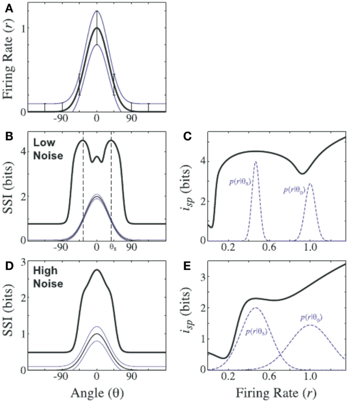
Figure 1. Stimulus specific surprise (i_sp) and stimulus specific information (i_SSI) of an orientation tuned model neuron under two different noise regimes. (A) Tuning curve: mean firing rate (thick line), SD (thin lines) versus stimulus orientation (Θ). Repeated in for (B,D) for clarity. (B) The stimulus specific information i_SSI (indicated as SSI) is maximal in regions of high slope of the tuning curve for the low noise case; (D) for the high noise case i_SSI (indicated as SSI) is maximal at the peak of the tuning curve. (C,E) The corresponding values of the stimulus specific surprise i_sp and the relevant conditional probability distributions. Figure reproduced from Butts and Goldman (2006). Creative Commons (CC BY) Attribution License.

3.2. Importance of the Stimulus Set and Response Features

It may not immediately be visible in the above equations, but central quantities of the above treatment, such as H(S), H(S|r) depend strongly on the choice of the stimulus set 𝒜_S. For example, if one chooses to study the human visual systems with a set of “visual” stimuli in the far infrared end of the spectrum, I(S : R) will most likely be very small and analysis futile (although done properly, a zero value of i_SSI(s : R) for all stimuli will correctly point out that the human visual system does not care or code for any of the infrared stimuli). Hence, characterizing a neural code properly hinges to a large extent on an appropriate choice of stimuli. In this respect, it is safe to assume that a move from artificial stimuli (such as gratings in visual neuroscience) to more natural ones will alter our view of neural codes in the future. A similar argument holds for the response features that are selected for analysis. If any feature is dropped or not measured at all this may distort the information measures above. This may even happen, if the dropped feature, say the exact spike time variable R_ST, seems to carry no mutual information with the stimulus variable when considered alone, i.e., I(S : R_ST) = 0. This is because there may still be synergistic information that can only be recovered by looking at other response variables jointly with R_ST. For example, it would be possible in principle that neither spike time R_ST nor spike rate R_SR carry mutual information with the stimulus variable when considered individually, i.e., I(S : R_ST) = I(S : R_SR) = 0. Still, when considered jointly they may be informative: I(S : R_ST, R_SR) > 0. The problem of omitted response features is almost inevitable in neuroscience, as the full sampling of all parts of a neural system is typically impossible, and we have to work with sub-sampled data. Considering only a subset of (response) variables may systematically alter the apparent dependency structure in the neural system [see Priesemann et al. (2009) for an example]. Therefore, the effects of subsampling should always be kept in mind when interpreting results of studies on neural coding. For many cases, however, it may in the future be possible to exploit regularities in the system, such as the decay of connection density between neurons, to model at least some missing parts of the overall response activity [e.g., by maximum entropy models (Tkacik et al., 2010; Granot-Atedgi et al., 2013; Priesemann et al., 2013b)].

4. Information in Ensemble Coding – Partial Information Decomposition

In neural systems, information is often encoded by ensembles of agents – as evidenced by the success of various “brain reading” and decoding techniques applied to multivariate neural data [e.g., Kriegeskorte et al. (2008)]. Knowing how this information in the ensemble is distributed over the agents can inform the designer of BICS about strategies to distribute the relevant information about a problem over the available agents. These strategies determine properties like the coding capacity of the system as well as its reliability. For example, reliability can be increased by representing the same information in multiple agents, making their information redundant. In contrast, maximizing capacity would require taking into account the full combinatorial possibilities of states of agents, making their coding synergistic.

Here, we investigate the most basic ensemble of just two agents to introduce the concepts of redundant, synergistic, and unique information (Williams and Beer, 2010; Stramaglia et al., 2012, 2014; Harder et al., 2013; Lizier et al., 2013; Barrett, 2014; Bertschinger et al., 2014; Griffith and Koch, 2014; Griffith et al., 2014; Timme et al., 2014), and note that encoding in larger ensembles is still a field of active research. More specifically, we consider an ensemble of two neurons and their responses {R₁, R₂}, after stimulation with stimuli s ∈ A_S = {s₁, s₂,…}, and try to answer the following questions:

1. What information does R_i provide about S? This is the mutual information I(S : R_i) between the responses of one neuron i and the stimulus set.

2. What information does the joint variable R = {R₁, R₂} provide about S? This is the mutual information I(S : R₁, R₂) between the joint responses of the two neurons and the stimulus set.

3. What information does the joint variable R = {R₁, R₂} have about S that we cannot get from observing both variables R₁, R₂ separately? This information is called the synergy, or complementary information, of {R₁, R₂} with respect to S: CI(S : R₁;R₂).

4. What information does one of the variables, say R₁, hold individually about S that we can not obtain from any other variable (R₂ in our case)? This information is the unique information of R₁ about S : UI(S : R₁∖R₂).

5. What information does one of the variables, again say R₁, have about S that we could also obtain by looking at the other variable alone? This information is the redundant, or shared, information of R₁ and R₂ about S: SI(S : R₁;R₂).

Interestingly, only questions 1 and 2 can be answered using standard tools of information theory such as the mutual information. In fact, the answers to the questions 3–5, i.e., the quantification of unique, redundant and synergistic information, need new mathematical concepts as will be shown below.

Before we present more details, we would like to illustrate the above questions by a thought experiment where three visual neurons are recorded simultaneously while being stimulated with a set of four stimuli (Figure 2). For simplicity, we will later consider the coding of these neurons with respect to questions 1–5 only in two pairwise configurations: one configuration composed of two neurons with almost identical receptive fields (RF₁, RF₂), another configuration of two neurons with collinear but spatially displaced receptive fields (RF₁, RF₃) (Figure 2A). These neurons are stimulated with one of the following stimuli (Figure 2B): s₁ does not contain anything at the receptive fields of the three neurons, and the neurons stay inactive; s₂ is a short bar in the receptive fields of neurons 1,2; s₃ is a similar short bar, but over the receptive field of neuron 3, instead of 1,2; s₄ is a long bar covering all receptive fields in the example.

FIGURE 2

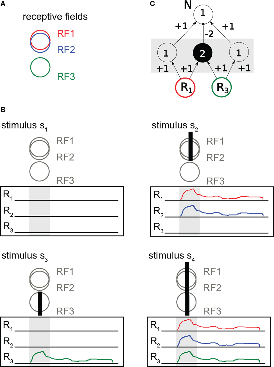
Figure 2. Redundant and synergistic neural coding. (A) Receptive fields (RFs) of three neurons R₁, R₂, and R₃. (B) Set of four stimuli. (C) Circuit for synergistic coding. Responses of neurons R₁, R₃ determine the response of neuron N via an XOR-function. In the hidden circuit in between R₁, R₂, and N open circles denote excitatory neurons, filled circles inhibitory neurons. Numbers in circles are activation thresholds, signed numbers at connecting arrows are synaptic weights.

To make things easy, let us encode responses that we get from these three neurons (colored traces in Figure 2B) in binary form, with a “1” simply indicating that there was a response in our response window (boxes with activity traces in Figure 2).

Classic information theory tells us that if we assume the stimuli to be presented with equal probability $\left(p\left(S=s_i\right)=\frac{1}{4},i=1,\dots 4\right),$ then the entropy of the stimulus set is H(S) = 2 (bit). Obviously, none of the information terms above can be larger than these 2 bits. We also see that each neuron shows activity (binary response = 1) in half of the cases, yielding an entropy H(R_j) = 1 for the responses of each neuron. The responses of the three neurons fully specify the stimulus, and therefore I(S : R₁, R₂, R₃) = 2. To see the mutual information between an individual neuron’s response and the stimulus we may compute I(S : R_i) = H(S) − H(S|R_i). To do this, we remember H(S) = 2 and use that the number of equiprobable outcomes for S drops by half after observing a single neuron (e.g., after observing a response r₁ = 1 of neuron 1, two stimuli remain possible sources of this response – s₂ or s₄). This gives H(S|R_i) = 1, and I(S : R_i) = 1. Hence, each neuron provides 1 bit of information about the stimulus when considered individually. Already here, we see something curious – although each of the three neurons has 1 bit about the stimulus, together they have only 2, not 3 bits. We can see the reason for this “vanishing bit” when considering responses from pairs of neurons, especially the pair {R₁, R₂}.

We now turn to questions 3–5, and ask about a decomposition of the information in joint variables formed from pairs of neurons:

• To understand the concept of redundant (or shared) information, consider the responses of neuron 1 and 2. These two neurons show identical responses to the stimuli. Individually, each of the neurons provides 1 bit of information about the stimulus. Jointly, i.e., if we look at them together ({R₁, R₂}), they still provide only 1 bit: I(S : R₁, R₂) = 1, not 2 bits. This is because the information carried by their responses is redundant. To see this, note that one cannot decide between stimuli s₁ and s₃ if one gets the result (r₁ = 0, r₂ = 0), and similarly one cannot not decide between stimuli s₂ and s₄ if one gets (r₁ = 1, r₂ = 1); other combinations of responses do not occur here. We see that neurons 1 and 2 have exactly the same information about the stimulus, and a measure of redundant information should yield the full 1 bit in this case². We will later see this intuitive argument again as the “Self-Redundancy” axiom (Williams and Beer, 2010).

• To understand the concept of synergy, consider the responses {R₁, R₃} from the second example pair (i.e., neurons 1,3), and ask how much information they have about the presence of exactly one short bar on the screen [i.e., s₂ or s₃, in contrast to a long bar (S₄) or no bar at all (s₁)]. Mathematically, the XOR function indicates whether a short bar is present or not, N = XOR (R₁, R₂). For a neural implementation of the XOR function, see Figure 2C. To examine synergy, we investigate the mutual information between {R₁, R₃}, R₁, R₃, and N. The individual mutual informations of each neuron R₁, R₃ with the downstream neuron N are zero [I(N : R_i) = 0]. However, the mutual information between these two neurons considered jointly and the downstream neuron N equals 1 bit, because the response of N is fully determined by its two inputs: I(N : R₁, R₃) = 1. Thus, there is only synergistic information between R₁ and R₃ about N, in this example about the presence of a single short bar.

• To understand the concept of unique information, consider only the neurons 1, 3 and the two stimuli s₁ and s₃. (The reduced stimulus set S′ is S′ = {s₁, s₃}). It is trivial to see that neuron 1 does not respond to either stimulus, thus the mutual information between neuron 1 and the reduced stimulus set is zero, I(S′ : R₁) = 0. In contrast, the responses of neuron 3 are fully informative about S′, I(S′ : R₃) = 1. Clearly, R₃ provides information about the stimulus that is not present in R₁. In this example, neuron 3 has 1 bit of unique information about the stimulus set S′.

We now introduce the mathematical framework of partial information decomposition that formalizes the intuition in the above examples. We consider a decomposition of the mutual information between a set of two right hand side, or input, variables R₁, R₂, and a left hand side variable, or output variable S, i.e., I(S : R₁, R₂). In general, for a decomposition of this mutual information into unique, redundant, and synergistic information to make sense, the total information from any one variable, e.g., I(S : R₁), should be decomposable into the unique information term UI(S : R₁∖R₂) and the redundant, or shared, information term SI(S : R₁;R₂) that both variables have about S:

$\begin{array}{ccc}\hfill I\left(S:R_1\right)& =\mathit{SI}\left(S:R_1;R_2\right)+\mathit{UI}\left(S:R_1\setminus R_2\right),\hfill & \hfill \\ \hfill I\left(S:R_2\right)& =\mathit{SI}\left(S:R_2;R_1\right)+\mathit{UI}\left(S:R_2\setminus R_1\right).\hfill \end{array}$ (22)

Similarly, the total information I(S : R₁, R₂) from both variables should be decomposable into the two unique information terms UI(S : R₁∖R₂) and UI(S : R₂∖R₁) of each R_i about S, the redundant, or shared, information SI(S : R₁;R₂) that both variables have about S, and the synergistic, or complementary, information CI(S : R₁;R₂) that can only be obtained by considering {R₁, R₂} jointly:

$I\left(S:R_1,R_2\right)=\mathit{UI}\left(S:R_1\setminus R_2\right)+\mathit{UI}\left(S:R_2\setminus R_1\right)+\mathit{SI}\left(S:R_1;R_2\right)+\mathit{CI}\left(S:R_1;R_2\right).$ (23)

Figure 3A shows this so-called partial information decomposition (Williams and Beer, 2010). One sees that the redundant, unique, and synergistic information cannot be obtained by simply subtracting classical mutual information terms. However, if we are given either a measure of redundant, synergistic, or unique information, the other parts of the decomposition can be computed. Hence, classic information theory is insufficient for a partial information decomposition (Williams and Beer, 2010), and a definition of either unique, redundant of synergistic information based on a choice of axioms is needed. A minimal requirement for such axioms, and measures satisfying them, is that they should comply with our intuitive notion of what unique, redundant, and synergistic information should be in some clear cut extreme cases, such as the examples above. The original set of axioms proposed for such a functional definition of redundant (and thereby also unique and synergistic) information comprises three axioms that currently all authors seem to agree on (Williams and Beer, 2010):

1. (Weak) Symmetry: the redundant information that variables R₁, R₂, …, R_n have about S is symmetric under permutations of the variables R₁, R₂, …, R_n.

2. Self-redundancy: the redundant information that R₁ shares with itself about S is just the mutual information I(S : R₁).

3. Monotonicity: the redundant information that variables R₁, R₂, …, R_n have about S is smaller than or equal to the redundant information that variables R₁, R₂, …, R_n−1 have about S. Equality holds if R_n−1 is a function of R_n.

FIGURE 3

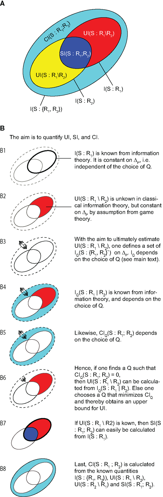
Figure 3. (A) Overview of the contributions to a partial information decompositions of the mutual information I(S:R1;R2). (B) (1–8) Schematic derivation of the definition of unique information by Bertschinger et al. (2014). This figure is meant as a guide to the structure of the original work that should be consulted for the rigorous treatment of the topic.

These three axioms also lead to global positivity, i.e., $\mathit{SI}\left(\cdot :\cdot \right)\ge 0,$$\mathit{CI}\left(\cdot :\cdot \right)\ge 0,$ and $\mathit{UI}\left(\cdot :\cdot \right)\ge 0$ (Williams and Beer, 2010). As said above, these axioms are uncontroversial, although some authors restrict them to only two input variables R₁, R₂ as detailed below (Harder et al., 2013; Rauh et al., 2014). These axioms, however, are not sufficient to uniquely define a measure of either redundant, unique or synergistic information. Therefore, various additional axioms, or assumptions, have been proposed (Williams and Beer, 2010; Harder et al., 2013; Lizier et al., 2013; Bertschinger et al., 2014; Griffith and Koch, 2014; Griffith et al., 2014) that are not all compatible with each other (Bertschinger et al., 2013). Here, we exemplarily discuss the recent choice of an assumption by Bertschinger et al. (2014) to define a measure of unique information, which is, in fact, equivalent to another formulation proposed by Griffith and Koch (2014). The reasons for selecting this particular assumption are that at the time of writing it comes with the richest set of derived theorems, and that it has an appealing link to game theory and utility functions, and thus to measures of success of an agent or a BICS. We note at the outset that this is one of the measures that are defined only for two “input” variables R₁, R₂ and one “output” S (although the R_i themselves may be multivariate RVs). For more details on this restriction see Rauh et al. (2014).

The basic idea of the definition by Bertschinger and colleagues comes from game theory and states that someone (say Alice) who has access to one input variable R₁ with unique information about an output variable S must be able to prove that her variable has information not available in the other. To prove this, Alice can design a bet on the output variable (by choosing a suitable utility function) so that someone else (say Bob) who has only access to the other input variable R₂ will on average loose this bet. Via some intermediate steps, this leads to the (defining) assumption that the unique information only depends on the two marginal probability distributions P(s, r₁) and P(s, r₂), but not on the exact full distribution P(s, r₁, r₂). In other words, the unique information UI should not change when replacing P with a probability distribution Q from the space Δ_p of probability distributions that share these marginals with P:

$\begin{array}{l}{\mathrm{\Delta }}_P=\{Q\in \mathrm{\Delta }:Q\left(S=s,R_1=r_1\right)=P\left(S=s,R_1=r_1\right)\\ \mathrm{and}Q\left(S=s,R_2=r_2\right)=P\left(S=s,R_2=r_2\right)\mathrm{for}\mathrm{all}s\in {\mathcal{A}}_S,r_1\in {\mathcal{A}}_{R_1},r_2\in {\mathcal{A}}_{R_2}\}\end{array}$ (24)

where Δ is the space of all probability distributions on the support of S, R₁, R₁. This motivated the following definition for a measure $\widetilde{UI}$ of unique information:

$\widetilde{\mathit{UI}}\left(S:R_1\setminus R_2\right)=\underset{Q\in {\mathrm{\Delta }}_P}{\mathit{min}}{I}_Q\left(S:R_1|R_2\right),$ (25)

where I_Q(S : R₁|R₂) is a conditional mutual information computed with respect to the joint distribution Q(s, r₁, r₂) instead of P(s, r₁, r₂). Note that this conditional mutual information I_Q(S : R₁|R₂) does change on Δ_p, and that only its minimum is a measure of the (constant) unique information (see Figure 3). As stated above, knowing one of the three parts UI, SI, CI is enough to compute the others. Therefore, the matching definitions of measures for redundant ($\widetilde{SI}$) and shared information ($\widetilde{CI}$) are:

$\widetilde{\mathit{SI}}\left(S:R_1;R_2\right)=\underset{Q\in {\mathrm{\Delta }}_P}{\mathit{max}}\mathit{Co}{I}_Q\left(S:R_1;R_2\right),$ (26)

$\widetilde{\mathit{CI}}\left(S:R_1;R_2\right)=I\left(S:R_1,R_2\right)-\underset{Q\in {\mathrm{\Delta }}_P}{\mathit{min}}{I}_Q\left(S:R_1,R_2\right).$ (27)

where CoI_Q(S;R₁;R₂) = I(S : R₁) − I_Q(S : R₁|R₂) is the so-called co-information (equivalent to the redundancy minus the synergy) for the distribution Q(s, r₁, r₂).

Among the notable properties of the measures defined this way is the fact that they can be found by convex optimization, and that all three measures above have been explicitly shown to be positive. Moreover, the above measures are bounds for any definitions of synergistic CI, shared (redundant) SI, and unique information UI that satisfy equations (22) and (23). That is, it can be shown that:

$\begin{array}{llll}\hfill \mathit{UI}\left(S:R_1\setminus R_2\right)& \le \widetilde{\mathit{UI}}\left(S:R_1\setminus R_2\right),& \hfill & \\ \hfill \mathit{UI}\left(S:R_2\setminus R_1\right)& \le \widetilde{\mathit{UI}}\left(S:R_2\setminus R_1\right),& \hfill & \\ \hfill \mathit{SI}\left(S:R_1;R_2\right)& \ge \widetilde{\mathit{SI}}\left(S:R_1;R_2\right),& \hfill & \\ \hfill \mathit{CI}\left(S:R_1;R_2\right)& \ge \widetilde{\mathit{CI}}\left(S:R_1;R_2\right),& \hfill & \end{array}$

holds (Bertschinger et al., 2014).

The field of information decomposition has seen a rapid development since the initial study of Williams and Beer; however, some major questions remain unresolved so far. Most importantly, the definitions above have acceptable properties, but apply only for the case of decomposing mutual information into contributions of two (sets of) input variables. The structure of such a decomposition for more than two inputs is an active area of research at the moment.

5. Analyzing Distributed Computation in Neural Systems

5.1. Analyzing Neural Coding and Goal Functions in a Domain-Independent Way

The analysis of neural coding strategies presented above relies on our a priori knowledge of the set of task level (e.g., stimulus) features that is encoded in neural responses at the implementation level. If we have this knowledge, information theory will help us to link the two levels. This is somewhat similar to the situation in cryptography where we consider a code “cracked” if we obtain a human-readable plain text message, i.e., we move from the implementation level (encrypted message) to the task level (meaning). However, what happens if the plain text were in a language that one never heard of³? In this case, we would potentially crack the code without ever realizing it, as the plain text still has no meaning for us.

The situation in neuroscience bears resemblance to this example in at least two respects: first, most neurons do not have direct access to any properties of the outside world, rather they receive nothing but input spike trains. All they ever learn and process must come from the structure of these input spike trains. Second, if we as researchers probe the system beyond early sensory or motor areas, we have little knowledge of what is actually encoded by the neurons deeper inside the system. As a result, proper stimulus sets get hard to choose. In this case, the gap between the task- and the implementation level may actually become too wide for meaningful analyses, as noticed recently by Carandini (2012).

Instead of relying on descriptions of the outside world (and thereby involve the task level), we may take the point of view that information processing in a neuron is nothing but the transformation of input spike trains to output spike trains. We may then try to use information theory to link the implementation and algorithmic level, by retrieving a “footprint” of the information processing carried out by a neural circuit. This approach only builds on a very general agreement that neural systems perform at least some kind of information processing. This information processing can be partitioned into the component processes, which determine or predict the next RV of a process Y at time t, Y_t: (1) information storage, (2) information transfer, and (3) information modification. A partition of this kind had already been formulated by Turing [see Langton (1990)], and was recently formalized by Lizier et al. (2014) [see also Lizier (2013)]:

• Information storage quantifies the information contained in the past state variable Y_t−1 of a process that is used by the process at the next RV at t, Y_t (Lizier et al., 2012b). This relatively abstract definition means that an observer will see at least a part of the past information in the process’ past again in its future, but potentially transformed. Hence, information storage can be naturally quantified by a mutual information between the past and the future⁴ of a process.

• Information transfer quantifies the information contained in the state variables X_t−u (found u time steps into the past) of one source process X that can be used to predict information in the future variable Y_t of a target process Y, in the context of the past state variables Y_t−1 of the target process (Schreiber, 2000; Paluš, 2001; Vicente et al., 2011).

• Information modification quantifies the combination of information from various source processes into a new form that is not trivially predictable from any subset of these source processes [for details of this definition also see Lizier et al. (2010, 2013)].

Based on Turing’s general partition of information processing (Langton, 1990), Lizier and colleagues recently proposed an information-theoretic framework to quantify distributed computations in terms of all three component processes locally, i.e., for each part of the system (e.g., neurons or brain areas) and each time step (Lizier et al., 2008c, 2010, 2012b). This framework is called local information dynamics and has been successfully applied to unravel computation in swarms (Wang et al., 2011), in Boolean networks (Lizier et al., 2011b), and in neural models (Boedecker et al., 2012) and data (Wibral et al., 2014a) (also see Section 6 for details on these example applications).

Crucially, information dynamics is the perspective of an observer who measures the processes X and Y and tries to partition the information in Y_t into the apparent contributions from stored, transferred, and modified information, without necessarily knowing the true underlying system structure. For example, such an observer would label any recurring information in Y as information storage, even where such information causally left the system and re-entered Y at a later time (e.g., a stigmergic process).

Other partitions are possible; James et al. (2011), for example, partition information in the present of a process in terms of its relationships to the semi-infinite past and semi-infinite future. In contrast, we focus on the information dynamics perspective laid out above since it quantifies terms, which can be specifically identified as information storage, transfer, and modification, which aligns with many qualitative descriptions of dynamics in complex systems. In particular, the information dynamics perspective is novel in focusing on quantifying these operations on a local scale in space and time.

In the following we present both global and local measures of information transfer, storage, and modification, beginning with the well established measures of information transfer and ending with the highly dynamic field of information modification.

5.2. Information Transfer

The analysis of information transfer was formalized initially by Schreiber (2000) and Paluš (2001), and has seen a rapid surge of interest in neuroscience⁵ and general physiology⁶. Information transfer as measured by the transfer entropy introduced below has recently also been given a thermodynamic interpretation by Prokopenko and Lizier (2014), continuing general efforts to link information theory and thermodynamics (Szilárd, 1929; Landauer, 1961), highlighting the importance of the concept.

5.2.1. Definition

Information transfer from a process X (the source) to another process Y (the target) is measured by the transfer entropy (TE) functional⁷ (Schreiber, 2000):

$\mathit{TE}\left({\mathbf{\text{X}}}_{t-u}\to Y_t\right)=I\left(X_{t-u}:Y_t|Y_{t-1}\right)$ (28)

$={\displaystyle \sum _{y_t\in {\mathcal{A}}_{Y_t,{\mathbf{\text{y}}}_{t-1}}\in {\mathcal{A}}_{{\mathbf{\text{Y}}}_{t-1},{\mathbf{\text{X}}}_{t-u}}\in {\mathcal{A}}_{{\mathbf{\text{X}}}_{t-u}}}}p\left(y_t,y_{t-1},x_{t-u}\right)\log \frac{p\left(y_t|y_{t-1},x_{t-u}\right)}{p\left(y_t|y_{t-1}\right)},$ (29)

where $I\left(\cdot :\cdot |\cdot \right)$ is the conditional mutual information, Y_t is the RV of process Y at time t, and X _t−u, Y _t−1 are the past state-RVs of processes X and Y, respectively. The delay variable u in X _t−u indicates that the past state of the source is to be taken u time steps into the past to account for a potential physical interaction delay between the processes. This parameter need not be chosen ad hoc, as it was recently proven for bivariate systems that the above estimator is maximized if the parameter u is equal to the true delay δ of the information transfer from X to Y (Wibral et al., 2013). This relationship allows one to estimate the true interaction delay δ from data by simply scanning the assumed delay u:

$\mathrm{\delta }=\underset{u}{\text{argmax}}\left[\mathit{TE}\left({\mathbf{\text{X}}}_{t-u}\to Y_t\right)\right]$ (30)

The TE functional can be linked to Wiener–Granger type causality (Wiener, 1956; Granger, 1969; Barnett et al., 2009). More precisely, for systems with jointly Gaussian variables, transfer entropy is equivalent⁸ to linear Granger causality [see Barnett et al. (2009) and references therein]. However, whether the assumption of jointly Gaussian variables is appropriate in a neural setting must be checked carefully for each case (note that Gaussianity of each marginal distribution is not sufficient). In fact, EEG source signals were found to be non-Gaussian (Wibral et al., 2008).

5.2.2. Transfer entropy estimation

When the probability distributions entering equation (28) are known (e.g., in an analytically tractable neural model), TE can be computed directly. However, in most cases, the probability distributions have to be derived from data. When probabilities are estimated naively from the data via counting, and when these estimates are then used to compute information-theoretic quantities such as the transfer entropy, we speak of a “plug in” estimator. Indeed, such plug in estimators has been used in the past, but they come with serious bias problems (Panzeri et al., 2007b). Therefore, newer approaches to TE estimation rely on a more direct estimation of the entropies that TE can be decomposed (Kraskov et al., 2004; Gomez-Herrero et al., 2010; Vicente et al., 2011; Wibral et al., 2014b). These estimators still suffer from bias problems but to a lesser degree (Kraskov et al., 2004). We therefore restrict our presentation to these approaches.

Before we can proceed to estimate TE we will have to reconstruct the states of the processes (see Section 2.1.5). One approach to state reconstruction is time delay embedding (Takens, 1981). It uses past variables X_{t− nτ}, n = 1, 2,… that are spaced in time by an interval τ. The number of these variables and their optimal spacing can be determined using established criteria (Ragwitz and Kantz, 2002; Small and Tse, 2004; Lindner et al., 2011; Faes et al., 2012). The realizations of the states variables can be represented as vectors of the form:

$x_t^d=\left(x_t,x_{t-\mathrm{\tau }},x_{t-\mathrm{2\tau }},...,x_{t-\left(d-1\right)\mathrm{\tau }}\right),$ (31)

where d is the dimension of the state vector. Using this vector notation, transfer entropy can be written as:

$\begin{array}{ccc}\hfill T{E}_{\mathit{SPO}}\left(X_{t-u}\to Y_t\right)& ={\displaystyle \sum _{y_t,{\mathbf{\text{y}}}_{t-1}^{d_y},{\mathbf{\text{x}}}_{t-u}^{d_x}}}p\left(y_t,y_{t-1}^{d_y},x_{t-u}^{d_x}\right)\hfill & \hfill \\ \hfill & \log \frac{p\left(y_t|y_{t-1}^{d_y},x_{t-u}^{d_x}\right)}{p\left(y_t|y_{t-1}^{d_y}\right)},\hfill \end{array}$ (32)

where the subscript SPO (for self prediction optimal) is a reminder that the past states of the target, $y_{t-1}^{d_y},$ have to be constructed such that conditioning on them is optimal in the sense of taking the active information storage in the target correctly into account (Wibral et al., 2013): if one were to condition on $y_{t-w}^{d_y}$ with w≠1, instead of $y_{t-1}^{d_y},$ then the self prediction for Y_t would not be optimal and the transfer entropy would be overestimated.

We can rewrite equation (32) using a representation in the form of four entropies⁹ H(⋅), as:

$\begin{array}{c}T{E}_{\mathit{SPO}}\left(X_{t-u}\to Y_t\right)=H\left(Y_{t-1}^{d_y},X_{t-u}^{d_x}\right)-H\left(y_t,Y_{t-1}^{d_y},X_{t-u}^{d_x}\right)\\ +H\left(y_t,Y_{t-1}^{d_y}\right)-H\left(Y_{t-1}^{d_y}\right).\end{array}$ (33)

Entropies can be estimated efficiently by nearest-neighbor techniques. These techniques exploit the fact that the distances between neighboring data points in a given embedding space are inversely related to the local probability density: the higher the local probability density around an observed data point the closer are the next neighbors. Since next neighbor estimators are data efficient (Kozachenko and Leonenko, 1987; Victor, 2005), they allow to estimate entropies in high-dimensional spaces from limited real data.

Unfortunately, it is problematic to estimate TE by simply applying a naive nearest-neighbor estimator for the entropy, such as the Kozachenko–Leonenko estimator (Kozachenko and Leonenko, 1987), separately to each of the terms appearing in equation (33). The reason is that the dimensionality of the state spaces involved in equation (33) differs largely across terms – creating bias problems. These are overcome by the Kraskov–Stögbauer–Grassberger (KSG) estimator that fixes the number of neighbors k in the highest dimensional space (spanned here by $y_t,y_{t-1}^{d_y},x_{t-u}^{d_x}$) and by projecting the resulting distances to the lower dimensional spaces as the range to look for additional neighbors there (Kraskov et al., 2004). After adapting this technique to the TE formula (Gomez-Herrero et al., 2010), the suggested estimator can be written as:

$T{E}_{\mathit{SPO}}\left(X_{t-u}\to Y_t\right)=\mathrm{\psi }\left(k\right)+⟨\mathrm{\psi }\left(n_{y_{t-1}^{d_y}}+1\right)-\mathrm{\psi }\left(n_{y_t{y}_{t-1}^{d_y}}+1\right)-\mathrm{\psi }\left(n_{y_{t-1}^{d_y}{x}_{t-u}^{d_x}}+1\right){⟩}_t,$ (34)

where ψ denotes the digamma function, the angle brackets (⟨⋅⟩_t) indicate averaging over time for stationary systems, or over an ensemble of replications for non-stationary ones, and k is the number of nearest neighbors used for the estimation. n_(⋅) refers to the number of neighbors, which are within a hypercube that defines the search range around a state vector. As described above, the size of the hypercube in each of the marginal spaces is defined based on the distance to the k-th nearest neighbor in the highest dimensional space.

5.2.3. Interpretation of transfer entropy as a measure at the algorithmic level

TE describes computation at the algorithmic level, not at the level of a physical dynamical system. As such it is not optimal for inference about causal interactions – although it has been used for this purpose in the past. The fundamental reason for this is that information transfer relies on causal interactions, but non-zero transfer entropy can occur without direct causal links, and causal interactions do not necessarily lead to non-zero information transfer (Ay and Polani, 2008; Lizier and Prokopenko, 2010; Chicharro and Ledberg, 2012). Instead, causal interactions may serve active information storage alone (see next section), or force two systems into identical synchronization, where information transfer becomes effectively zero. This might be summarized by stating that transfer entropy is limited to effects of a causal interaction from a source to a target process that are unpredictable given the past of the target process alone. In this sense, TE may be seen as quantifying causal interactions currently in use for the communication aspect of distributed computation. Therefore, one may say that TE measures predictive, or algorithmic information transfer.

A simple thought experiment may serve to illustrate this point: when one plays an unknown record, a chain of causal interactions serve the transfer of information about the music from the record to your brain. Causal interactions happen between the record’s grooves and the needle, the magnetic transducer system behind the needle, and so on, up to the conversion of pressure modulations to neural signals in the cochlea that finally activate your cortex. In this situation, there undeniably is information transfer, as the information read out from the source, the record, at any given moment is not yet known in the target process, i.e., the neural activity in the cochlea. However, this information transfer ceases if the record has a crack, making the needle skip, and repeat a certain part of the music. Obviously, no new information is transferred which under certain mild conditions is equivalent to no information transfer at all. Interestingly, an analysis of TE between sound and cochlear activity will yield the same result: the repetitive sound leads to repetitive neural activity (at least after a while). This neural activity is thus predictable by its own past, under the condition of vanishing neural “noise,” leaving no room for a prediction improvement by the sound source signal. Hence, we obtain a TE of zero, which is the correct result from a conceptual point of view. Remarkably, at the same time the chain of causal interactions remains practically unchanged. Therefore, a causal model able to fit the data from the original situation will have no problem to fit the data of the situation with the cracked record, as well. Again, this is conceptually the correct result, but this time from a causal point of view.

The difference between an analysis of information transfer in a computational sense and causality analysis based on interventions has been demonstrated convincingly in a recent study by Lizier and Prokopenko (2010). The same authors also demonstrated why an analysis of information transfer can yield better insight than the analysis of causal interactions if the computation in the system is to be understood. The difference between causality and information transfer is also reflected in the fact that a single causal structure can support diverse pattern of information transfer (functional multiplicity), and the same pattern of information transfer can be realized with different causal structures (structural degeneracy) as shown by Battaglia (2014b).

5.2.4. Local information transfer

As transfer entropy is formally just a conditional mutual information, we can obtain the corresponding local conditional mutual information [equation (15)] from equation (32). This quantity is called the local transfer entropy (Lizier et al., 2008c). For realizations x_t, y_t of two processes X, Y at time t it reads:

$\mathit{te}\left(X_{t-u}=x_{t-u}\to Y_t=y_t\right)=\log \frac{p\left(y_t|y_{t-1}^{d_y},x_{t-u}^{d_x}\right)}{p\left(y_t|y_{t-1}^{d_y}\right)},$ (35)

As said earlier in the section on basic information theory, the use of local information measures does not eliminate the need for an appropriate estimation of the probability distributions involved. Hence, for a non-stationary process, these distributions will still have to be estimated via an ensemble approach for each time point for the RVs involved, e.g., via physical replications of the system, or via enforcing cyclostationarity by design of the experiment.

The analysis of local transfer entropy has been applied with great success in the study of cellular automata to confirm the conjecture that certain coherent spatiotemporal structures traveling through the network are indeed the main carriers of information transfer (Lizier et al., 2008c) (see further discussion at Section 6.4). Similarly, local transfer entropy has identified coherent propagating wave structures in flocks as information cascades (Wang et al., 2012) (see Section 6.5), and indicated impending synchronization among coupled oscillators (Ceguerra et al., 2011).

5.2.5. Common problems and solutions

Typical problems in TE estimation encompass (1) finite sample bias, (2) the presence of non-stationarities in the data, and (3) the need for multivariate analyses. In recent years, all of these problems have been addressed at least in isolation, as summarized below:

• Finite sample bias can be overcome by statistical testing using surrogate data, where the observed realizations $y_t,y_{t-1}^{d_y},x_{t-u}^{d_x}$ of the RVs $Y_t,Y_{t-1}^{d_y},X_{t-u}^{d_x}$ are reassigned to other RVs of the process, such that the temporal order underlying the information transfer is destroyed [for an example see the procedures suggested in Lindner et al. (2011)]. This reassignment should conserve as many data features of the single process realizations as possible.

• As already explained in the section on basic information theory above, non-stationary random processes in principle require that the necessary estimates of the probabilities in equation (28) are based on physical replications of the systems in question. Where this is impossible, the experimenter should design the experiment in such a way that the processes are repeated in time. If such cyclostationary data are available, then TE should be estimated using ensemble methods as described in Gomez-Herrero et al. (2010) and implemented in the TRENTOOL toolbox (Lindner et al., 2011; Wollstadt et al., 2014).

• So far, we have restricted our presentation of transfer entropy estimation to the case of just two interacting random processes X, Y, i.e., a bivariate analysis. In a setting that is more realistic for neuroscience, one deals with large networks of interacting processes X, Y, Z, …. In this case, various complications arise if the analysis is performed in a bivariate manner. For example, a process Z could transfer information with two different delays δ_Z→X, δ_Z→Y to two other processes X, Y. In this case, a pairwise analysis of transfer entropy between X, Y will yield an apparent information transfer from the process that receives information from Z with the shorter delay to the one that receives it with the longer delay (common driver effect). A similar problem arises if information is transferred first from a process X to Y, and then from Y to Z. In this case, a bivariate analysis will also indicate information transfer from X to Z (cascade effect). Moreover, two sources may transfer information purely synergistically, i.e., the transfer entropy from each source alone to the target is zero, and only considering them jointly reveals the information transfer¹⁰.

From a mathematical perspective, this problem seems to be easily solved by introducing the complete transfer entropy, which is defined in terms of a conditional transfer entropy (Lizier et al., 2008c, 2010):

$\mathit{TE}\left(X_{t-u}\to Y_t|Z^{-}\right)={\displaystyle \sum _{y_t,{\mathbf{\text{y}}}_{\mathbf{\text{t}}-1},{\mathbf{\text{x}}}_{\mathbf{\text{t}}-\mathbf{\text{u}}},{\mathbf{\text{z}}}^{-}}}p\left(y_t,y_{t-1},x_{t-u},z^{-}\right)\log \frac{p\left(y_t|y_{t-1},x_{t-u},z^{-}\right)}{p\left(y_t|y_{t-1},z^{-}\right)},$ (36)

where the state-RV Z⁻ is a collection of the past states of one or more processes in the network other than X, Y. We label equation (36) a complete transfer entropy TE^(c)(X_t−u →Y_t) when we take Z⁻ = V⁻, the set of all processes in the network other than X, Y.

It is important to note that TE and conditional/complete TE are complementary (see mathematical description of this at Section 5.4) – each can reveal aspects of the underlying dynamics that the other does not and both are required for a full description. While conditional TE removes redundancies and includes synergies, knowing that redundancy is present may be important, and local pairwise TE additionally reveals interesting cases when a source is mis-informative about the dynamics (Lizier et al., 2008b,c).

Furthermore, even for small networks of random processes the joint state space of the variables Y_t, Y_t−1, X_t−u, V⁻ may become intractably large from an estimation perspective. Moreover, the problem of finding all information transfers in the network, either from single sources variables into the target or synergistic transfer from collections of source variables to the target, is a combinatorial problem, and can therefore typically not be solved in a reasonable time.

Therefore, Faes et al. (2012), Lizier and Rubinov (2012), and Stramaglia et al. (2012) suggested to analyze the information transfer in a network iteratively, selecting information sources for a target in each iteration either based on magnitude of apparent information transfer (Faes et al., 2012) or its significance (Lizier and Rubinov, 2012; Stramaglia et al., 2012). In the next iteration, already selected information sources are added to the conditioning set [Z⁻ in equation (36)], and the next search for information sources is started. The approach of Stramaglia and colleagues is particular here in that the conditional mutual information terms are computed at each level as a series expansion, following a suggestion by Bettencourt et al. (2008). This allows for an efficient computation as the series may truncate early, and the search can proceed to the next level. Importantly, these approaches also consider synergistic information transfer from more than one source variable to the target. For example, a variable transferring information purely synergistically with Z⁻ maybe included in the next iteration, given that the other variables it transfers information with are already in the conditioning set Z⁻. However, there is currently no explicit indication in the approaches of Faes et al. (2012) and Lizier and Rubinov (2012) as to whether multivariate information transfer from a set of sources to the target is, in fact, synergistic; in addition, redundant links will not be included. In contrast, both redundant and synergistic multiplets of variables transferring information into a target may be identified in the approach of Stramaglia et al. (2012) by looking at the sign of the contribution of the multiplet. Unfortunately, there is also the possibility of cancellation if both types of multivariate information (redundant, synergistic) are present.

5.3. Active Information Storage

Before we present explicit measures of active information storage, a few comments may serve to avoid misunderstanding. Since we analyze neural activity here, measures of active information storage are concerned with information stored in this activity – rather than in synaptic properties, for example¹¹. This is the perspective of what an observer of that activity (not necessarily with any knowledge of the underlying system structure) would attribute as information storage at the algorithmic level, even if the causal mechanisms at the level of a physical dynamical system underpinning such apparent storage were distributed externally to the given variable (Lizier et al., 2012b). As laid out above, storage is conceptualized here as a mutual information between past and future states of neural activity. From this it is clear that there will not be much information storage if the information contained in the future states of neural activity is low in general. If, on the other hand these future states are rich in information but bear no relation to past states, i.e., are unpredictable, again information storage will be low. Hence, large information storage occurs for activity that is rich in information but, at the same time, predictable.

Thus, information storage gives us a way to define the predictability of a process that is independent of the prediction error: information storage quantifies how much future information of a process can be predicted from its past, whereas the prediction error measures how much information can not be predicted. If both are quantified via information measures, i.e., in bits, the error and the predicted information add up to the total amount of information in a random variable of the process. Importantly, these two measures may lead to quite different views about the predictability of a process. This is because the total information can vary considerably over the process, and the predictable and the unpredictable information may thus vary almost independently. This is important for the design of BICS that use predictive coding strategies.

Before turning to the explicit definition of measures of information storage it is worth considering which temporal extent of “past” and “future” states we are interested in: most globally, predictive information (Bialek et al., 2001) or excess entropy (Crutchfield and Packard, 1982; Grassberger, 1986; Crutchfield and Feldman, 2003) is the mutual information between the semi-infinite past and semi-infinite future of a process before and after time point t. In contrast, if we are interested in the information currently used for the next step of the process, the mutual information between the semi-infinite past and the next step of the process, the active information storage (Lizier et al., 2012b) is of greater interest. Both measures are defined in the next paragraphs.

5.3.1. Predictive information/excess entropy

Excess entropy is formally defined as:

$E_{X_t}=\underset{k\to \infty }{\lim }I\left(X_t^{k-}:X_t^{k+}\right)$ (37)

where $X_t^{k-}=\left\{X_t,X_{t-1},\dots ,X_{t-k+1}\right\},$ and $X_t^{k+}=\{X_{t+1},\dots$, $X_{t+k}\}$ indicate collections of the past and future k variables of the process X ¹². These collections of RVs $\left(X_t^{k-},X_t^{k+}\right),$ in the limit k →∞, span the semi-infinite past and future, respectively. In general, the mutual information in equation (37) has to be evaluated over multiple realizations of the process. For stationary processes, however, $E_{X_t}$ is not time-dependent, and equation (37) can be rewritten as an average over time points t and computed from a single realization of the process – at least in principle (we have to consider that the process must run for an infinite time to allow the limit $\underset{k\to \infty }{lim}$for all t):

$E_X={⟨\underset{k\to \infty }{\lim }i\left(x_t^{k-}:x_t^{k+}\right)⟩}_t.$ (38)

Here, $i\left(\cdot :\cdot \right)$ is the local mutual information from equation (14), and $x_t^{k-},x_t^{k+}$ are realizations of $X_t^{k-},X_t^{k+}.$ The limit of k →∞ can be replaced by a finite k_max if a k_max exists such that conditioning on $X_t^{k_{\mathit{max}}-}$ renders $X_t^{k_{\mathit{max}}+}$ conditionally independent of any X_l with l ≤ t − k_max.

Even if the process in question is non-stationary, we may look at values that are local in time as long as the probability distributions are derived appropriately (see Section 2.1.2) (Shalizi, 2001; Lizier et al., 2012b):

$e_{X_t}=\underset{k\to \infty }{lim}i\left(x_t^{k-}:x_t^{k+}\right).$ (39)

5.3.2. Active Information Storage

From a perspective of the dynamics of information processing, we might not be interested in information that is used by a process at some time far in the future, but at the next point in time, i.e., information that is said to be “currently in use” for the computation of the next step (the realization of the next RV) in the process (Lizier et al., 2012b). To quantify this information, a different mutual information is computed, namely the active information storage (AIS) (Lizier et al., 2007, 2012b):

$A_{X_t}=\underset{k\to \infty }{\lim }I\left(X_{t-1}^{k-}:X_t\right).$ (40)

AIS is similar to a measure called “regularity” introduced by Porta et al. (2000), and was also labeled as ρ_u (“redundant portion” of information in X_t) by James et al. (2011).

Again, if the process in question is stationary then $A_{X_t}=\mathrm{const}.=A_X$ and the expected value can be obtained from an average over time – instead of an ensemble of realizations of the process – as:

$A_X={⟨\underset{k\to \infty }{\lim }i\left(x_{t-1}^{k-}:x_t\right)⟩}_t,$ (41)

which can be read as an average over local active information storage (LAIS) values $a_{X_t}$ (Lizier et al., 2012b):

$A_X={⟨a_{X_t}⟩}_t$ (42)

$a_{X_t}=\underset{k\to \infty }{\lim }i\left(x_{t-1}^{k-}:x_t\right).$ (43)

Even for non-stationary processes, we may investigate local active storage values, given the corresponding probability distributions are properly obtained from an ensemble of realizations of X_t, $X_{t-1}^{k-}$:

$a_{X_t}=\underset{k\to \infty }{\lim }i\left(x_{t-1}^{k-}:x_t\right).$ (44)

Again, the limit of k →∞ can be replaced by a finite k_max if a k_max exists such that conditioning on $X_{t-1}^{k_{\mathit{max}}}$ renders X_t conditionally independent of any X_l with l ≤ t − k_max [see equation (16)].

5.3.3. Interpretation of information storage as a measure at the algorithmic level

As laid out above information storage is a measure of the amount of information in a process that is predictable from its past. As such it quantifies, for example, how well activity in one brain area A can be predicted by another area, e.g., by learning its statistics. Hence, questions about information storage arise naturally when asking about the generation of predictions in the brain, e.g., in predictive coding theories (Rao and Ballard, 1999; Friston et al., 2006).

5.4. Combining the Analysis of Local Active Information Storage and Local Transfer Entropy

The two measures of local active information storage and local transfer entropy introduced in the preceding section may be fruitfully combined by pairing storage and transfer values at each point in time and for each agent. The resulting space has been termed the “local information dynamics state space” and has been used to investigate the computational capabilities of cellular automata, by pairing a(y_j,t) and te(x_i,t−1 →y_j,t) for each pair of source and target x_i, y_j at each time point (Lizier et al., 2012a).

Here, we suggest that this concept may be used to disentangle various neural processing strategies. Specifically we suggest to pair the sum¹³ over all local active information storage in the inputs x_i of a target y_j [at the relevant delays u_i, obtained from an analysis of transfer entropy (Wibral et al., 2013)] with the sum of outgoing local information transfers from this target to further targets z_k, for each agent y_j and each time point t:

$\left({\displaystyle \sum _{x_i}}a\left(x_{i,t-u_i}\right),{\displaystyle \sum _{z_k}}\mathit{te}\left(y_{j,t}\to z_{k,t+u_k}\right)\right)$ (45)

where sources x_i and second order targets z_k are defined by the conditions:

$\mathit{te}\left(x_{i,t-u_i}\to y_{j,t}\right)\ne 0,\forall x_{i,t-u_i}$ (46)

$\mathit{te}\left(y_{j,t}\to z_{k,t+u_k}\right)\ne 0,\forall z_{k,t+u_k}.$ (47)

The resulting point set can be used to answer the important question, whether the aggregate outgoing information transfer of an agent is high either for predictable or for surprising input. The former information processing function amounts to a sort of filtering, passing on reliable (predictable) information, and would be linked to something reliable being represented in activity. The latter information processing function is a form of prediction error encoding, where high outgoing information transfer is triggered when surprising, unpredictable information is received (also see Figure 4).

FIGURE 4

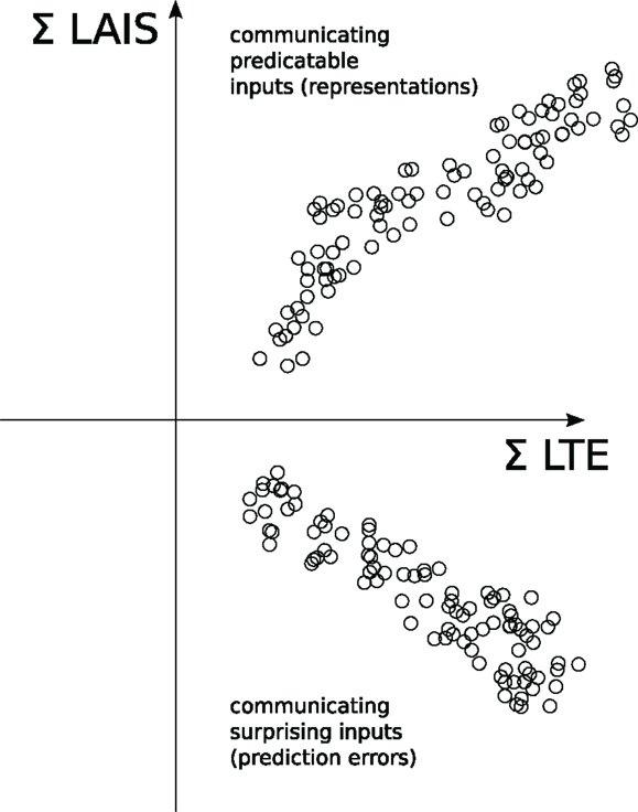
Figure 4. Various information processing regimes in the information state space. ΣLAIS = sum of local active information storage in input, ΣLTE = sum of outgoing local transfer entropy. Each dot represents these values for one agent and time step.

Note that for this type of analysis recordings of at least triplets of connected agents are necessary. This may pose a considerable challenge in experimental neuroscience, but may be extremely valuable to disentangle the information processing goal functions of the various cortical layers, for example. This type of analysis will also be valuable to understand the information processing in evolved BICS, as in these systems the availability of data from triplets of agents is no problem.

5.5. Information Modification and Its Relation to Partial Information Decomposition

Langton (1990) described information modification as an interaction between transmitted and/or stored information that results in a modification of one or the other. Attempts to define information modification more rigorously implemented this basic idea. First attempts at defining a quantitative measure of information modification resulted in a heuristic measure termed local separable information (Lizier et al., 2010), where the local active information storage and the sum over all pairwise local transfer entropies into the target was taken:

$s_{X_t}=a_{X_t}+{\displaystyle \sum _{{\mathbf{\text{Z}}}_{t^{-},i}\in {\mathbf{\text{V}}}_{X_t}\backslash {\mathbf{\text{X}}}_{t-1}}}i\left(x_t:z_{t^{-},i}|x_{t-1}\right),$ (48)

with $V_{X_t}\setminus X_{t-1}=\left\{Z_{t^{-},1},\dots ,Z_{t^{-},G}\right\}$ indicating the set of G past state variables of all processes $Z_{t^{-},i}$ that transfer information into the target variable X_t; note that X_t−1, the history of the target, is explicitly not part of the set. The index t⁻ is a reminder that only past state variables are taken into account, i.e., t⁻ < t. As shown above, the local measures entering the sum are negative if they are mis-informative about the future of the target. Eventually the overall sum, or separable information, might also be negative, indicating that neither the pairwise information transfers, nor the history could explain the information contained in the target’s future. This has been interpreted as a modification of either stored or transferred information.

While this first attempt provided valuable insights in systems like elementary cellular automata (Lizier et al., 2010), it is ultimately heuristic. A more rigorous approach is to look at decomposition of the local information h(x_t) in the realization of a random variable to shed some more light on the issue which part of this information may be due to modification. In this view, the overall information H(X_t), in the future of the target process [or its local form, h(x_t)] can be explained by looking at all sources of information and the history of the target jointly, at least up to the remaining stochastic part (the intrinsic innovation of the random process) in the target, as shown by Lizier et al. (2010) [also see equations (50) and (51)]. In contrast, we cannot decompose this information into pairwise mutual information terms only. As described in the following, the remainder after exhausting pairwise terms is due to synergistic information between information sources and has motivated the suggestion to define information modification based on synergy (Lizier et al., 2013).

To see the differences between a partition considering variables jointly or only in pairwise terms, consider a series of subsets formed from the set of all variables $Z_{t^{-},i}$ (defined above; ordered by i here) that can transfer information into the target, except variables from the target’s own history. The bold typeface in $Z_{t^{-},i}$ is a reminder that we work with a state space representation where necessary. Following the derivation by Lizier et al. (2010), we create a series of subsets $V_{X_t}^g\setminus X_{t-1}$ such that $V_{X_t}^g\setminus X_{t-1}=\left\{Z_{t^{-},1},\dots ,Z_{t^{-},g-1}\right\},$ i.e., the g-th subset only contains the first g − 1 sources. We can decompose the collective transfer entropy from all our source variables, $\mathit{TE}\left(V_{X_t}\setminus X_{t-1}\to X_t\right),$ as a series of conditional mutual information terms, incrementally increasing the set that we condition on:

$\mathit{TE}\left(V_{X_t}\setminus X_{t-1}\to X_t\right)={\displaystyle \sum _{g=1}^G}I\left(X_t:Z_{t^{-},g}|X_{t-1},V_{X_t}^g\setminus X_{t-1}\right).$ (49)

These conditional MI terms are all transfer entropies – starting for g = 1 with a pairwise transfer entropy $\mathit{TE}\left(Z_{t^{-},1}\to X_t\right),$ then with conditional transfer entropies for g = 2…G − 1 and finishing with a complete transfer entropy for g = G, $\mathit{TE}\left(Z_{t^{-},G}\to X_t|V_{X_t}^G\setminus X_{t-1}\right).$ The total entropy of the target H(X_t) can then be written as:

$H\left(X_t\right)=A_{X_{t-1}}+{\displaystyle \sum _{g=1}^G}I\left(X_t:Z_{t^{-},g}|X_{t-1},V_{X_t}^g\setminus X_{t-1}\right)+W_{X_t}$ (50)

where $W_{X_t}$ is the innovation in X_t. If we rewrite the partition in equation (50) in its local form:

$h\left(x_t\right)=a_{X_{t-1}}+{\displaystyle \sum _{g=1}^G}i\left(x_t:z_{t^{-},g}|x_{t-1},v_{X_t}^g\setminus x_{t-1}\right)+w_{X_t},$ (51)

and compare to equation (48), we see that the difference between the potentially mis-informative sum $s_{X_t}$ in equation (48) and the fully accounted for information in h(x_t) from equation (51) lies in the conditioning of the local transfer entropies. This means that the context that the source variables provide for each other is neglected and synergies and redundancies (see Section 4) are not properly accounted for. Importantly, the results of both equations (48) and (51) are identical, if no information is provided either redundantly or synergistically by the sources $Z_{t^{-},g}.$ This observation led Lizier et al. (2013) to propose a more rigorously defined measure of information modification based on the synergistic part of the information transfer from the source variables $Z_{t^{-},g},$ and the targets history X_t−1 to the target X_t. This definition of information modification has several highly desirable properties. However, it relies on a suitable definition of synergy, which is currently only available for the case of two source variables (see Section 4). As there is currently a considerable debate on how to define the part of a the mutual information I(Y : {X₁, …, X_i,…}), which is synergistically provided by a larger set of source variables X_i [but see Gomez-Herrero et al. (2010)], the question of how to best measure information modification may still be considered open.

6. Application Examples

6.1. Active Information Storage in Neural Data

Here, we present two very recent applications of (L)AIS to neural data and their estimation strategies for the PDFs. In both, estimation of (L)AIS was done using the JAVA information dynamics toolkit (Lizier, 2012c, 2014b) and state space reconstruction was performed in TRENTOOL (Lindner et al., 2011) [for details, see Gomez et al. (2014) and Wibral et al. (2014a)]. The first study investigated AIS in magnetoencephalographic (MEG) source signals from patients with autism spectrum disorder (ASD), and reported a reduction of AIS in the hippocampus in patients compared to healthy controls (Gomez et al., 2014) (Figure 5). In this study, the strategy for obtaining an estimate of the PDF was to use only baseline data (between stimulus presentations) to guarantee stationarity of the data. Results from this study align well with predictive coding theories (Rao and Ballard, 1999; Friston et al., 2006) of ASD [also see Gomez et al. (2014), and references therein]. The significance of this study in the current context lies in the fact, which it explicitly sought to measure the information processing consequences at the algorithmic level of changes in neural dynamics in ASD at the implementation level.

FIGURE 5

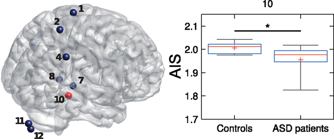
Figure 5. AIS in ASD patients compared to controls. (Left) Investigated MEG source locations (spheres; red = significantly lower AIS in ASD, blue = not sign.). (Right) Box and whisker plot for LAIS in source 10 (Hippocampus, corresponding to red sphere), where significant differences in AIS between patients and controls were found. Modified from Gomez et al. (2014); creative commons attribution license (BB CY 3.0).

The second study (Wibral et al., 2014a) analyzed LAIS in voltage sensitive dye (VSD) imaging data from cat visual cortex. The study found low LAIS in the baseline before the onset of a visual stimulus, negative LAIS directly after stimulus onset and sustained increases in LAIS for the whole stimulation period, despite changing raw signal amplitude (Figure 6). These observed information profiles constrain the set of possible underlying algorithms being implemented in the cat’s visual cortex. In this study, all available data were pooled, both from baseline and stimulation periods, and also across all recording sites (VSD image pixels). Pooling across time is unusual, but reasonable insofar as neurons themselves also have to deal with non-stationarities as they arise, and a measure of neurally accessible LAIS should reflect this. Pooling across all sites in this study was motivated by the argument that all neural pools seen by VSD pixels are capable of the same dynamic transitions as they were all in the same brain area. Thus, pixels were treated as physical replications for the estimation of the PDF. In sum, the evaluation strategy of this study is applicable to non-stationary data, but delivers results that strongly depend on the data included. Its future application therefore needs to be informed by precise estimates of the time scales at which neurons may sample their input statistics.

FIGURE 6

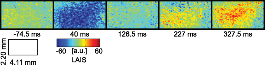
Figure 6. LAIS in VSD data from cat visual cortex (area 18), before and after presentation of a visual stimulus at time t = 0 ms. Modified from Wibral et al. (2014a); creative commons attribution license (BB CY 3.0).

6.2. Active Information Storage in a Robotic System

Recurrent neural networks (RNNs) consist of a reservoir of nodes or artificial neurons connected in some recurrent network structure (Maass et al., 2002; Jaeger and Haas, 2004). Typically, this structure is constructed at random, with only the output neurons connections trained to perform a given task. This approach is becoming increasingly popular for non-linear time-series modeling and robotic applications (Boedecker et al., 2012; Dasgupta et al., 2013). The use of Intrinsic Plasticity based techniques (Schrauwen et al., 2008) is known to assist performance of such RNNs in general, although this method is still outperformed on memory capacity tasks, for example, by the implementation of certain changes to the network structure (Boedecker et al., 2009).

To address this issue, Dasgupta et al. (2013) add an on-line rule to adapt the “leak-rate” of each neuron based on the AIS of its internal state. The leak-rate is reduced where the AIS is below a certain threshold, and increased where it is above. The technique was shown to improve performance on delayed memory tasks, both for benchmark tests and in embodied wheeled and hexapod robots. Dasgupta et al. (2013) describe the effect of their technique as speeding up or slowing down the dynamics of the reservoir based on the time-scale(s) of the input signal. In terms of Marr’s levels, we can also view this as an intervention at the algorithmic level, directly adjusting the level of information storage in the system in order to affect the higher-level computational goal of enhanced performance on memory capacity tasks. It is particularly interesting to note the connection in information storage features across these different levels here.

6.3. Balance of Information Processing Capabilities Near Criticality

It has been conjectured that the brain may operate in a self-organized critical state (Beggs and Plenz, 2003), and recent evidence demonstrates that the human brain is at least very close to criticality, albeit slightly sub-critical (Priesemann et al., 2013a, 2014). This prompts the question of what advantages would be delivered by operating in such a critical state. From a dynamical systems perspective, one may suggest that the balance of stability (from ordered dynamics) with perturbation spreading (from chaotic dynamics) in this regime (Langton, 1990) gives rise to the scale-free correlations and emergent structures that we associate with computation in natural systems. From an information dynamics perspective, one may suggest that the critical regime represents a balance between capabilities of information storage and information transfer in the system, with too much of either one decaying the ability for emergent structures to carry out the complementary function (Langton, 1990; Lizier et al., 2008b, 2011b).

Several studies have upheld this interpretation of maximized but balanced information processing properties near the critical regime. In a study of random Boolean networks it was shown that TE and AIS are in an optimal balance near the critical point (Lizier et al., 2008b, 2011b). This is echoed by findings for recurrent neural networks (Boedecker et al., 2012) and for maximization of transfer entropy in the Ising model (Barnett et al., 2013), and maximization of entropy in neural models and recordings (Haldeman and Beggs, 2005; Shew and Plenz, 2013). From Marr’s perspective, we see here that at the algorithmic level the optimal balance of these information processing operations yields the emergent and scale-free structures associated with the critical regime at the implementation level. This reflects the ties between Marr’s levels as described in Section 6.2. These theoretical findings on computational properties at the critical point are of great relevance to neuroscience, due to the aforementioned importance of criticality in this field.

6.4. Local Information Dynamics in Cellular Automata

Cellular automata (CAs) are discrete dynamical systems with an array of cells that synchronously update their value as a function of a fixed number of spatial neighbors cells, using a uniform rule (Wolfram, 2002). CAs are a classic complex system where, despite their simplicity, emergent structures arise. These include gliders, which are coherent structures moving against regular background domains. These gliders and their interactions have formed the basis of analysis of cellular automata as canonical examples of nature-inspired distributed information processing (e.g., in a distributed “density” classification process to determine whether the initial state had a majority of “1” or “0” states) (Mitchell, 1998). In particular (moving), gliders were conjectured to transmit information across the CA, static gliders to store information, and their collisions or interactions to process information in “computing” new macro-scale dynamics of the CA.

Local transfer entropy, active information storage and separable information were applied to CAs to produce spatiotemporal local information dynamics profiles in a series of experiments (Lizier et al., 2008c, 2010, 2012b; Lizier, 2013, 2014a). The results of these experiments confirmed the long-held conjectures that gliders are the dominant information transfer entities in CAs, while blinkers and background domains are the dominant information storage components, and glider/particle collisions are the dominant information modification events. These results are crucial in demonstrating the alignment between our qualitative understanding of emergent information processing in complex systems and our new ability to quantify such information processing via these measures. These insights could only be gained by using local information measures, as studying averages alone tells us nothing about the presence of these spatiotemporal structures.

For our purposes, a crucial step was the extension of this analysis to a CA rule (known as ψ_par), which was evolved to perform the density classification task outlined above (Lizier, 2013; Lizier et al., 2014), since we may interpret this with Marr’s levels (Section 2.2). Spatiotemporal profiles of local information dynamics for a sample run of this density classification rule are shown in Figure 7, and may be reproduced using the DemoFrontiersBitsFromBiology2014.m script in the demos/octave/CellularAutomata demonstration distributed with the Java Information Dynamics Toolkit (Lizier, 2014b). In this example, the classification of the density of the initial CA state is the clear goal of the computation (task level). At the algorithmic level, our local information dynamics analysis allowed direct identification of the roles of the emergent structures arising on the CA after a short initial transient Figure 7. For example, this analysis revealed markers that CA regions had identified local majorities of “0” or “1” (see the wholly white or black regions, or checkerboard patterns indicating uncertainty). These regions are identified as storing this information in Figure 7B. The analysis also quantifies the role of several glider types in communicating the presence of these local majorities and the strength of those majorities (see the slow and faster glider structures identified as information transfer in Figures 7C,D), and the role of glider collisions resolving competing local majorities.

FIGURE 7

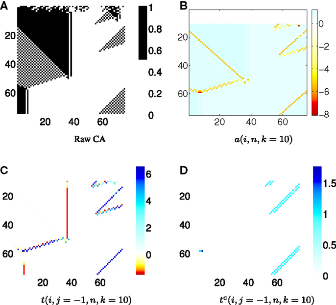
Figure 7. Local information dynamics in rule ψ_par. Local information dynamics in rule ψ_par with r = 3 for the raw values displayed in (A) (black for “1,” white for “0”). Seventy-five time steps are displayed for 75 cells, starting from an initial random state. Notice that a short initial transient occurs after that the emergent structures arise. For the spatiotemporal information dynamics plots (B–D), we use a history length k = 10 (therefore, the measures are undefined and not plotted for n ≤ 10), and all units are in bits. We have (B) Local active information storage a(i, n, k = 10); (C) Local apparent or pairwise transfer entropy one cell to the left t(i, j = − 1, n, k = 10); and (D) Local complete transfer entropy one cell to the left t^c(i, j = − 1, n, k = 10). After Lizier et al. (2014).

6.5. Information Cascades in Swarms and Flocks

Swarming or flocking refers to the collective behavior exhibited in movement by a group of animals (Lissaman and Shollenberger, 1970; Parrish and Edelstein-Keshet, 1999), including the emergence of patterns and structures such as cascades of perturbations traveling in a wave-like manner, splitting, and reforming of groups and group avoidance of obstacles. Such behavior is thought to provide biological advantages, e.g., protection from predators. Realistic simulation of swarm behavior can be generated using three simple rules for individuals in the swarm, based on separation, alignment, and cohesion with others (Reynolds, 1987).

Wang et al. (2012) analyzed the local information storage and transfer dynamics exhibited in the patterns of motion in a swarm model, based on time-series of (relative) headings and speeds of each individual. Most importantly, this analysis quantitatively revealed the coherent cascades of motion in the swarm as waves of large, coherent information transfer [as had previously been conjectured, e.g., see Couzin et al. (2006) and Bikhchandani et al. (1992)].

These “information cascades” are analogous to the gliders in CAs (above), and strongly constrain the possible algorithms being implemented in the swarm here. When viewed using Marr’s levels they have a similar algorithmic role of carrying information coherently and efficiently across the swarm, while the implementation of the information here is simply in the relative heading and speed of the individuals. The goal of the computation (task level) for the swarm depends on the current environment, but may be to avoid predators, or efficiently transport the whole group to nesting or food sites.

6.6. Transfer Entropy Guiding Self-Organization in a Snakebot

Lizier et al. (2008a) inverted the usual use of transfer entropy, applying it for the first time as a fitness function in the evolution of adaptive behavior, as an example of guided self-organization (Prokopenko, 2009, 2014). This experiment utilized a snakebot – a snake-like robot with separately controlled modules along its body, whose individual actuation was evolved via genetic programing to maximize transfer entropy between adjacent modules. The actual motion of the snake emerged from the interaction between the modules and their environment. While the approach did not result in a particularly fast-moving snake (as had been hypothesized), it did result in coherent traveling information waves along the snake, which were revealed only by local transfer entropy.

These coherent information waves are akin to gliders in CAs and cascades in swarms (above), suggesting that such waves may emerge as a resonant mode in evolution for information flow. This may be because they are robust and optimal for coherent communication over long distances, and may be simple to construct via evolutionary steps. Again, we may use Marr’s levels here to identify the goal of the computation (task level) as to transfer information between the snake’s modules here (perhaps information about the terrain encountered). At the algorithmic level, the coherent waves carry this information efficiently along the snake’s whole body, while the implementation is simply in the attempted actuation of the modules on joints and their interaction (tempered by the environment).

7. Conclusion and Outlook

Neural systems perform acts of information processing in the form of distributed (biological) computation, and many of the more complex computations and emergent information processing capabilities remain mysterious to date. Information theory can help to advance our understanding in two ways.

On the one hand, neural information processing can be quantitatively partitioned into its component processes of information storage, transfer, and modification using information-theoretic tools (Section 5). These observations allow us to derive constraints on possible algorithms served by the observed neural dynamics. That is to say, these measures of how information is processed allow us to narrow in on the algorithm(s) being implemented in the neural system. Importantly, this can be done without necessarily understanding the underlying causal structure precisely.

On the other hand, the representations that these algorithms operate on, can be guessed by analyzing the mutual information between human-understandable descriptions of relevant concepts and quantities in our experiments and indices of neural activity (Section 3). This helps to identify which parts of the real world neural systems care for. However, care must be taken when asking such questions about neural codes or representations, as the separation of how neurons code uniquely, redundantly, and synergistically has not been solved completely to date (Section 4).

Taken together, the knowledge about representations and possible algorithms describes the operational principles of neural systems at Marr’s algorithmic level. Such information-theoretic insights may hint at solutions for solving ill-defined real world problems that biologically inspired computing systems have to face with their constrained resources.

Author Contributions

VP, MW, and JL wrote and critically revised the manuscript.

Conflict of Interest Statement

The Review Editor Michael Harre declares that, despite having collaborated with author Joseph T. Lizier, the review process was handled objectively and no conflict of interest exists. The authors declare that the research was conducted in the absence of any commercial or financial relationships that could be construed as a potential conflict of interest.

Acknowledgments

We thank Patricia Wollstadt and Lucas Rudelt for proof reading of the manuscript. Funding: MW was supported by LOEWE-Grant “Neuronale Koordination Forschungsschwerpunkt Frankfurt.” VP received financial support from the German Ministry for Education and Research (BMBF) via the Bernstein Center for Computational Neuroscience (BCCN) Göttingen under Grant No. 01GQ1005B.

Footnotes

1. ^Called the “computational level” by Marr originally. This terminology, however, collides with other meanings of computation used in this text.
2. ^Note that the fact that both neurons have the same amount of information (1 bit) is not sufficient in general for redundancy, although it is in this special case, as 1 bit is also the mutual information between the responses considered jointly and the stimuli.
3. ^See, for example, the Navajo code during World War Two that was never deciphered (Fox, 2014).
4. ^We consider ourselves having information up to time t−1, predicting the future values at t.
5. ^Paluš (2001), Chávez et al. (2003), Hadjipapas et al. (2005), Leistritz et al. (2006), Gourevitch and Eggermont (2007), Barnett et al. (2009), Garofalo et al. (2009), Sabesan et al. (2009), Staniek and Lehnertz (2009), Buehlmann and Deco (2010), Besserve et al. (2010a,b), Li and Ouyang (2010), Lüdtke et al. (2010), Vakorin et al. (2009, 2010, 2011), Amblard and Michel (2011), Ito et al. (2011), Lindner et al. (2011), Lizier et al. (2011a), Neymotin et al. (2011), Vicente et al. (2011); Wibral et al. (2011), Battaglia et al. (2012), Stetter et al. (2012), Bedo et al. (2014), Butail et al. (2014), Battaglia (2014a), Chicharro (2014), Kawasaki et al. (2014), Liu and Pelowski (2014), Marinazzo et al. (2014a,b,c), McAuliffe (2014), Montalto et al. (2014), Orlandi et al. (2014), Porta et al. (2014), Razak and Jensen (2014), Rowan et al. (2014), Shimono and Beggs (2014), Thivierge (2014), Untergehrer et al. (2014), van Mierlo et al. (2014), Varon et al. (2014), Yamaguti and Tsuda (2014), Zubler et al. (2014).
6. ^Faes and Nollo (2006), Faes et al. (2011a,b, 2014a,b), Faes and Porta (2014).
7. ^A functional maps from the relevant probability distribution (i.e., functions) to the real numbers. In contrast, an estimator maps from empirical data, i.e., a set of real numbers, to the real numbers.
8. ^To a constant factor of 2.
9. ^For continuous-valued RVs, these entropies are differential entropies.
10. ^Again, cryptography may serve as an example here. If an encrypted message is received, there will be no discernible information transfer from encrypted message to plain text without the key. In the same way, there is no information transfer from the key alone to the plain text. It is only when encrypted message and key are combined that the relation between the combination of encrypted message and key on the one side and the plain text on the other side is revealed.
11. ^See the distinction made between passive storage in synaptic properties and active storage in dynamics by Zipser et al. (1993).
12. ^In principle, these could harness embedding delays, as defined in equation (31)
13. ^More complex ways of combining incoming active information storage are conceivable.

References

Amblard, P. O., and Michel, O. J. (2011). On directed information theory and Granger causality graphs. J. Comput. Neurosci. 30, 7–16. doi: 10.1007/s10827-010-0231-x

Pubmed Abstract | Pubmed Full Text | CrossRef Full Text | Google Scholar

Ay, N., and Polani, D. (2008). Information flows in causal networks. Adv. Complex Syst. 11, 17. doi:10.1142/S0219525908001465

CrossRef Full Text | Google Scholar

Barnett, L., Barrett, A. B., and Seth, A. K. (2009). Granger causality and transfer entropy are equivalent for Gaussian variables. Phys. Rev. Lett. 103, 238701. doi:10.1103/PhysRevLett.103.238701

Pubmed Abstract | Pubmed Full Text | CrossRef Full Text | Google Scholar

Barnett, L., Lizier, J. T., Harré, M., Seth, A. K., and Bossomaier, T. (2013). Information flow in a kinetic Ising model peaks in the disordered phase. Phys. Rev. Lett. 111, 177203. doi:10.1103/PhysRevLett.111.177203

Pubmed Abstract | Pubmed Full Text | CrossRef Full Text | Google Scholar

Barrett, A. B. (2014). An exploration of synergistic and redundant information sharing in static and dynamical Gaussian systems. arXiv:1411.2832.

Google Scholar

Battaglia, D. (2014a). “Function follows dynamics: state-dependency of directed functional influences,” in Directed Information Measures in Neuroscience eds M. Wibral, R. Vicente, and J. T. Lizier (Heidelberg: Springer), 111–135. doi:10.1007/978-3-642-54474-3

CrossRef Full Text | Google Scholar

Battaglia, D. (2014b). “Function follows dynamics: state-dependency of directed functional influences,” in Directed Information Measures in Neuroscience (Understanding Complex Systems), eds M. Wibral, R. Vicente, and J. T. Lizier (Berlin: Springer), 111–135.

Google Scholar

Battaglia, D., Witt, A., Wolf, F., and Geisel, T. (2012). Dynamic effective connectivity of inter-areal brain circuits. PLoS Comput. Biol. 8:e1002438. doi:10.1371/journal.pcbi.1002438

Pubmed Abstract | Pubmed Full Text | CrossRef Full Text | Google Scholar

Bedo, N., Ribary, U., and Ward, L. M. (2014). Fast dynamics of cortical functional and effective connectivity during word reading. PLoS ONE 9:e88940. doi:10.1371/journal.pone.0088940

Pubmed Abstract | Pubmed Full Text | CrossRef Full Text | Google Scholar

Beggs, J. M., and Plenz, D. (2003). Neuronal avalanches in neocortical circuits. J. Neurosci. 23, 11167–11177.

Pubmed Abstract | Pubmed Full Text | Google Scholar

Bertschinger, N., Rauh, J., Olbrich, E., and Jost, J. (2013). “Shared information—new insights and problems in decomposing information in complex systems,” in Proceedings of the European Conference on Complex Systems 2012, eds T. Gilbert, M. Kirkilionis, and G. Nicolis (Springer), 251–269. doi:10.1007/978-3-319-00395-5_35

CrossRef Full Text | Google Scholar

Bertschinger, N., Rauh, J., Olbrich, E., Jost, J., and Ay, N. (2014). Quantifying unique information. Entropy 16, 2161–2183. doi:10.3390/e16042161

CrossRef Full Text | Google Scholar

Besserve, M., Scholkopf, B., Logothetis, N. K., and Panzeri, S. (2010a). Causal relationships between frequency bands of extracellular signals in visual cortex revealed by an information theoretic analysis. J. Comput. Neurosci. 29, 547–566. doi:10.1007/s10827-010-0236-5

Pubmed Abstract | Pubmed Full Text | CrossRef Full Text | Google Scholar

Besserve, M., Schölkopf, B., Logothetis, N. K., and Panzeri, S. (2010b). Causal relationships between frequency bands of extracellular signals in visual cortex revealed by an information theoretic analysis. J. Comput. Neurosci. 29, 547–566. doi:10.1007/s10827-010-0236-5

Pubmed Abstract | Pubmed Full Text | CrossRef Full Text | Google Scholar

Bettencourt, L. M., Gintautas, V., and Ham, M. I. (2008). Identification of functional information subgraphs in complex networks. Phys. Rev. Lett. 100, 238701. doi:10.1103/PhysRevLett.100.238701

CrossRef Full Text | Google Scholar

Bialek, W., Nemenman, I., and Tishby, N. (2001). Predictability, complexity, and learning. Neural Comput. 13, 2409–2463. doi:10.1162/089976601753195969

Pubmed Abstract | Pubmed Full Text | CrossRef Full Text | Google Scholar

Bikhchandani, S., Hirshleifer, D., and Welch, I. (1992). A theory of fads, fashions, custom, and cultural change as informational cascades. J. Polit. Econ. 100, 992–1026. doi:10.1086/261849

CrossRef Full Text | Google Scholar

Boedecker, J., Obst, O., Lizier, J. T., Mayer, N. M., and Asada, M. (2012). Information processing in echo state networks at the edge of chaos. Theory Biosci. 131, 205–213. doi:10.1007/s12064-011-0146-8

Pubmed Abstract | Pubmed Full Text | CrossRef Full Text | Google Scholar

Boedecker, J., Obst, O., Mayer, N. M., and Asada, M. (2009). Initialization and self-organized optimization of recurrent neural network connectivity. HFSP J. 3, 340–349. doi:10.2976/1.3240502

Pubmed Abstract | Pubmed Full Text | CrossRef Full Text | Google Scholar

Buehlmann, A., and Deco, G. (2010). Optimal information transfer in the cortex through synchronization. PLoS Comput. Biol. 6:e1000934. doi:10.1371/journal.pcbi.1000934

Pubmed Abstract | Pubmed Full Text | CrossRef Full Text | Google Scholar

Butail, S., Ladu, F., Spinello, D., and Porfiri, M. (2014). Information flow in animal-robot interactions. Entropy 16, 1315–1330. doi:10.3390/e16031315

CrossRef Full Text | Google Scholar

Butts, D. A. (2003). How much information is associated with a particular stimulus? Network 14, 177–187. doi:10.1088/0954-898X/14/2/301

Pubmed Abstract | Pubmed Full Text | CrossRef Full Text | Google Scholar

Butts, D. A., and Goldman, M. S. (2006). Tuning curves, neuronal variability, and sensory coding. PLoS Biol. 4:e92. doi:10.1371/journal.pbio.0040092

Pubmed Abstract | Pubmed Full Text | CrossRef Full Text | Google Scholar

Carandini, M. (2012). From circuits to behavior: a bridge too far? Nat. Neurosci. 15, 507–509. doi:10.1038/nn.3043

Pubmed Abstract | Pubmed Full Text | CrossRef Full Text | Google Scholar

Ceguerra, R. V., Lizier, J. T., and Zomaya, A. Y. (2011). “Information storage and transfer in the synchronization process in locally-connected networks,” in 2011 IEEE Symposium on Artificial Life (ALIFE) (Paris: IEEE), 54–61.

Google Scholar

Chávez, M., Martinerie, J., and Le Van Quyen, M. (2003). Statistical assessment of nonlinear causality: application to epileptic EEG signals. J. Neurosci. Methods 124, 113–128. doi:10.1016/S0165-0270(02)00367-9

Pubmed Abstract | Pubmed Full Text | CrossRef Full Text | Google Scholar

Chicharro, D. (2014). “Parametric and non-parametric criteria for causal inference from time-series,” in Directed Information Measures in Neuroscience (Springer), 195–219.

Google Scholar

Chicharro, D., and Ledberg, A. (2012). When two become one: the limits of causality analysis of brain dynamics. PLoS ONE 7:e32466. doi:10.1371/journal.pone.0032466

Pubmed Abstract | Pubmed Full Text | CrossRef Full Text | Google Scholar

Couzin, I. D., James, R., Croft, D. P., and Krause, J. (2006). “Social organization and information transfer in schooling fishes,” in Fish Cognition and Behavior (Fish and Aquatic Resources), eds C. Brown, K. N. Laland, and J. Krause (New York: Blackwell Publishing), 166–185.

Google Scholar

Crowley, K., and Siegler, R. S. (1993). Flexible strategy use in young children’s tic-tac-toe. Cogn. Sci. 17, 531–561. doi:10.1207/s15516709cog1704_3

CrossRef Full Text | Google Scholar

Crutchfield, J. P., and Feldman, D. P. (2003). Regularities unseen, randomness observed: levels of entropy convergence. Chaos 13, 25–54. doi:10.1063/1.1530990

Pubmed Abstract | Pubmed Full Text | CrossRef Full Text | Google Scholar

Crutchfield, J. P., and Packard, N. (1982). Symbolic dynamics of one-dimensional maps: entropies, finite precision, and noise. Int. J. Theor. Phys. 21, 433–466. doi:10.1007/BF02650178

CrossRef Full Text | Google Scholar

Dasgupta, S., Wörgötter, F., and Manoonpong, P. (2013). Information dynamics based self-adaptive reservoir for delay temporal memory tasks. Evol. Syst. 4, 235–249. doi:10.1007/s12530-013-9080-y

CrossRef Full Text | Google Scholar

Dewdney, A. (1989). A tinkertoy computer that plays tic-tac-toe. Scientific American 120–121.

Google Scholar

DeWeese, M. R., and Meister, M. (1999). How to measure the information gained from one symbol. Network 10, 325–340. doi:10.1088/0954-898X/10/4/303

Pubmed Abstract | Pubmed Full Text | CrossRef Full Text | Google Scholar

Faes, L., Marinazzo, D., Montalto, A., and Nollo, G. (2014a). Lag-specific transfer entropy as a tool to assess cardiovascular and cardiorespiratory information transfer. IEEE Trans. Biomed. Eng. 61, 2556–2568. doi:10.1109/TBME.2014.2323131

Pubmed Abstract | Pubmed Full Text | CrossRef Full Text | Google Scholar

Faes, L., Nollo, G., Jurysta, F., and Marinazzo, D. (2014b). Information dynamics of brain – heart physiological networks during sleep. New J. Phys. 16, 105005. doi:10.1088/1367-2630/16/10/105005

CrossRef Full Text | Google Scholar

Faes, L., and Nollo, G. (2006). Bivariate nonlinear prediction to quantify the strength of complex dynamical interactions in short-term cardiovascular variability. Med. Biol. Eng. Comput. 44, 383–392. doi:10.1007/s11517-006-0043-3

Pubmed Abstract | Pubmed Full Text | CrossRef Full Text | Google Scholar

Faes, L., Nollo, G., and Porta, A. (2011a). Information-based detection of nonlinear granger causality in multivariate processes via a nonuniform embedding technique. Phys. Rev. E Stat. Nonlin. Soft Matter Phys. 83(5 Pt 1), 051112. doi:10.1103/PhysRevE.83.051112

Pubmed Abstract | Pubmed Full Text | CrossRef Full Text | Google Scholar

Faes, L., Nollo, G., and Porta, A. (2011b). Non-uniform multivariate embedding to assess the information transfer in cardiovascular and cardiorespiratory variability series. Comput. Biol. Med. 42, 290–297. doi:10.1016/j.compbiomed.2011.02.007

Pubmed Abstract | Pubmed Full Text | CrossRef Full Text | Google Scholar

Faes, L., Nollo, G., and Porta, A. (2012). Non-uniform multivariate embedding to assess the information transfer in cardiovascular and cardiorespiratory variability series. Comput. Biol. Med. 42, 290–297. doi:10.1016/j.compbiomed.2011.02.007

Pubmed Abstract | Pubmed Full Text | CrossRef Full Text | Google Scholar

Faes, L., and Porta, A. (2014). “Conditional entropy-based evaluation of information dynamics in physiological systems,” in Directed Information Measures in Neuroscience (Springer), 61–86.

Google Scholar

Fano, R. (1961). Transmission of Information. Cambridge, MA: The MIT Press.

Google Scholar

Fox, M. (2014). Chester nez, 93, dies; navajo words washed from mouth helped win war. The New York Times.

Google Scholar

Friston, K., Kilner, J., and Harrison, L. (2006). A free energy principle for the brain. J. Physiol. Paris 100, 70–87. doi:10.1016/j.jphysparis.2006.10.001

CrossRef Full Text | Google Scholar

Gardner, W. A. (1994). “An introduction to cyclostationary signals,” in Cyclostationarity in Communications and Signal Processing, ed. W. A. Garnder (New York: IEEE Press), 1–90.

Google Scholar

Gardner, W. A., Napolitano, A., and Paura, L. (2006). Cyclostationarity: half a century of research. Signal Processing 86, 639–697. doi:10.1016/j.sigpro.2005.06.016

CrossRef Full Text | Google Scholar

Garofalo, M., Nieus, T., Massobrio, P., and Martinoia, S. (2009). Evaluation of the performance of information theory-based methods and cross-correlation to estimate the functional connectivity in cortical networks. PLoS ONE 4:e6482. doi:10.1371/journal.pone.0006482

Pubmed Abstract | Pubmed Full Text | CrossRef Full Text | Google Scholar

Gomez, C., Lizier, J. T., Schaum, M., Wollstadt, P., Grützner, C., Uhlhaas, P., et al. (2014). Reduced predictable information in brain signals in autism spectrum disorder. Front. Neuroinformatics 8:9. doi:10.3389/fninf.2014.00009

Pubmed Abstract | Pubmed Full Text | CrossRef Full Text | Google Scholar

Gomez-Herrero, G., Wu, W., Rutanen, K., Soriano, M. C., Pipa, G., and Vicente, R. (2010). Assessing coupling dynamics from an ensemble of time series. arXiv:1008.0539.

Google Scholar

Gourevitch, B., and Eggermont, J. J. (2007). Evaluating information transfer between auditory cortical neurons. J. Neurophysiol. 97, 2533–2543. doi:10.1152/jn.01106.2006

Pubmed Abstract | Pubmed Full Text | CrossRef Full Text | Google Scholar

Granger, C. W. J. (1969). Investigating causal relations by econometric models and cross-spectral methods. Econometrica 37, 424–438. doi:10.2307/1912791

CrossRef Full Text | Google Scholar

Granot-Atedgi, E., Tkacik, G., Segev, R., and Schneidman, E. (2013). Stimulus-dependent maximum entropy models of neural population codes. PLoS Comput. Biol. 9:e1002922. doi:10.1371/journal.pcbi.1002922

Pubmed Abstract | Pubmed Full Text | CrossRef Full Text | Google Scholar

Grassberger, P. (1986). Toward a quantitative theory of self-generated complexity. Int. J. Theor. Phys. 25, 907–938. doi:10.1007/BF00668821

CrossRef Full Text | Google Scholar

Griffith, V., Chong, E. K. P., James, R. G., Ellison, C. J., and Crutchfield, J. P. (2014). Intersection information based on common randomness. Entropy 16, 1985–2000. doi:10.3390/e16041985

CrossRef Full Text | Google Scholar

Griffith, V., and Koch, C. (2014). “Quantifying synergistic mutual information,” in Guided Self-Organization: Inception, Volume 9 of Emergence, Complexity and Computation, ed. M. Prokopenko (Berlin: Springer), 159–190.

Google Scholar

Hadjipapas, A., Hillebrand, A., Holliday, I. E., Singh, K. D., and Barnes, G. R. (2005). Assessing interactions of linear and nonlinear neuronal sources using meg beamformers: a proof of concept. Clin. Neurophysiol. 116, 1300–1313. doi:10.1016/j.clinph.2005.01.014

Pubmed Abstract | Pubmed Full Text | CrossRef Full Text | Google Scholar

Haldeman, C., and Beggs, J. M. (2005). Critical branching captures activity in living neural networks and maximizes the number of metastable states. Phys. Rev. Lett. 94, 058101. doi:10.1103/PhysRevLett.94.058101

CrossRef Full Text | Google Scholar

Harder, M., Salge, C., and Polani, D. (2013). Bivariate measure of redundant information. Phys. Rev. E Stat. Nonlin. Soft Matter Phys. 87, 012130. doi:10.1103/PhysRevE.87.012130

Pubmed Abstract | Pubmed Full Text | CrossRef Full Text | Google Scholar

Havenith, M. N., Yu, S., Biederlack, J., Chen, N.-H., Singer, W., and Nikolić, D. (2011). Synchrony makes neurons fire in sequence, and stimulus properties determine who is ahead. J. Neurosci. 31, 8570–8584. doi:10.1523/JNEUROSCI.2817-10.2011

Pubmed Abstract | Pubmed Full Text | CrossRef Full Text | Google Scholar

Ito, S., Hansen, M. E., Heiland, R., Lumsdaine, A., Litke, A. M., and Beggs, J. M. (2011). Extending transfer entropy improves identification of effective connectivity in a spiking cortical network model. PLoS ONE 6:e27431. doi:10.1371/journal.pone.0027431

Pubmed Abstract | Pubmed Full Text | CrossRef Full Text | Google Scholar

Jaeger, H., and Haas, H. (2004). Harnessing nonlinearity: predicting chaotic systems and saving energy in wireless communication. Science 304, 78–80. doi:10.1126/science.1091277

Pubmed Abstract | Pubmed Full Text | CrossRef Full Text | Google Scholar

James, R. G., Ellison, C. J., and Crutchfield, J. P. (2011). Anatomy of a bit: information in a time series observation. Chaos 21, 037109. doi:10.1063/1.3637494

Pubmed Abstract | Pubmed Full Text | CrossRef Full Text | Google Scholar

Johansson, R. S., and Birznieks, I. (2004). First spikes in ensembles of human tactile afferents code complex spatial fingertip events. Nat. Neurosci. 7, 170–177. doi:10.1038/nn1177

Pubmed Abstract | Pubmed Full Text | CrossRef Full Text | Google Scholar

Kawasaki, M., Uno, Y., Mori, J., Kobata, K., and Kitajo, K. (2014). Transcranial magnetic stimulation-induced global propagation of transient phase resetting associated with directional information flow. Front. Hum. Neurosci. 8:173. doi:10.3389/fnhum.2014.00173

Pubmed Abstract | Pubmed Full Text | CrossRef Full Text | Google Scholar

Knill, D. C., and Pouget, A. (2004). The Bayesian brain: the role of uncertainty in neural coding and computation. Trends Neurosci. 27, 712–719. doi:10.1016/j.tins.2004.10.007

Pubmed Abstract | Pubmed Full Text | CrossRef Full Text | Google Scholar

Kozachenko, L., and Leonenko, N. (1987). Sample estimate of entropy of a random vector. Probl. Info. Transm. 23, 95–100.

Google Scholar

Kraskov, A., Stoegbauer, H., and Grassberger, P. (2004). Estimating mutual information. Phys. Rev. E Stat. Nonlin. Soft Matter Phys. 69(6 Pt 2), 066138. doi:10.1103/PhysRevE.69.066138

Pubmed Abstract | Pubmed Full Text | CrossRef Full Text | Google Scholar

Kriegeskorte, N., Mur, M., Ruff, D. A., Kiani, R., Bodurka, J., Esteky, H., et al. (2008). Matching categorical object representations in inferior temporal cortex of man and monkey. Neuron 60, 1126–1141. doi:10.1016/j.neuron.2008.10.043

Pubmed Abstract | Pubmed Full Text | CrossRef Full Text | Google Scholar

Landauer, R. (1961). Irreversibility and heat generation in the computing process. IBM J. Res. Dev. 5, 183–191. doi:10.1073/pnas.1219672110

Pubmed Abstract | Pubmed Full Text | CrossRef Full Text | Google Scholar

Langton, C. G. (1990). Computation at the edge of chaos: phase transitions and emergent computation. Physica D 42, 12–37. doi:10.1016/0167-2789(90)90064-V

CrossRef Full Text | Google Scholar

Leistritz, L., Hesse, W., Arnold, M., and Witte, H. (2006). Development of interaction measures based on adaptive non-linear time series analysis of biomedical signals. Biomed. Tech. (Berl) 51, 64–69. doi:10.1515/BMT.2006.012

Pubmed Abstract | Pubmed Full Text | CrossRef Full Text | Google Scholar

Li, X., and Ouyang, G. (2010). Estimating coupling direction between neuronal populations with permutation conditional mutual information. Neuroimage 52, 497–507. doi:10.1016/j.neuroimage.2010.05.003

Pubmed Abstract | Pubmed Full Text | CrossRef Full Text | Google Scholar

Lindner, M., Vicente, R., Priesemann, V., and Wibral, M. (2011). Trentool: a Matlab open source toolbox to analyse information flow in time series data with transfer entropy. BMC Neurosci. 12:119. doi:10.1186/1471-2202-12-119

Pubmed Abstract | Pubmed Full Text | CrossRef Full Text | Google Scholar

Lissaman, P. B. S., and Shollenberger, C. A. (1970). Formation flight of birds. Science 168, 1003–1005. doi:10.1126/science.168.3934.1003

CrossRef Full Text | Google Scholar

Liu, T., and Pelowski, M. (2014). A new research trend in social neuroscience: towards an interactive-brain neuroscience. Psych J. 3, 177–188. doi:10.1002/pchj.56

CrossRef Full Text | Google Scholar

Lizier, J. (2014a). “Measuring the dynamics of information processing on a local scale in time and space,” in Directed Information Measures in Neuroscience, eds M. Wibral, R. Vicente, and J. T. Lizier (Berlin: Springer), 161–193. Understanding Complex Systems.

Google Scholar

Lizier, J. T. (2012c). JIDT: An Information-Theoretic Toolkit for Studying the Dynamics of Complex Systems. Available at: http://code.google.com/p/information-dynamics-toolkit/

Google Scholar

Lizier, J. T. (2013). The Local Information Dynamics of Distributed Computation in Complex Systems. Springer Theses, Springer, Berlin.

Google Scholar

Lizier, J. T. (2014b). JIDT: an information-theoretic toolkit for studying the dynamics of complex systems. Front. Robot. AI 1:11. doi:10.3389/frobt.2014.00011

CrossRef Full Text | Google Scholar

Lizier, J. T., Flecker, B., and Williams, P. L. (2013). “Towards a synergy-based approach to measuring information modification,” in 2013 IEEE Symposium on Artificial Life (ALIFE) (Singapore: IEEE), 43–51.

Google Scholar

Lizier, J. T., Heinzle, J., Horstmann, A., Haynes, J.-D., and Prokopenko, M. (2011a). Multivariate information-theoretic measures reveal directed information structure and task relevant changes in fMRI connectivity. J. Comput. Neurosci. 30, 85–107. doi:10.1007/s10827-010-0271-2

Pubmed Abstract | Pubmed Full Text | CrossRef Full Text | Google Scholar

Lizier, J. T., Pritam, S., and Prokopenko, M. (2011b). Information dynamics in small-world Boolean networks. Artif. Life 17, 293–314. doi:10.1162/artl_a_00040

Pubmed Abstract | Pubmed Full Text | CrossRef Full Text | Google Scholar

Lizier, J. T., and Prokopenko, M. (2010). Differentiating information transfer and causal effect. Eur. Phys. J. B 73, 605–615. doi:10.1140/epjb/e2010-00034-5

CrossRef Full Text | Google Scholar

Lizier, J. T., Prokopenko, M., Tanev, I., and Zomaya, A. Y. (2008a). “Emergence of glider-like structures in a modular robotic system,” in ALIFE, eds S. Bullock, J. Noble, R. Watson, and M. A. Bedau (Cambridge, MA: MIT Press), 366–373.

Google Scholar

Lizier, J. T., Prokopenko, M., and Zomaya, A. Y. (2008b). “The information dynamics of phase transitions in random Boolean networks,” in Proceedings of the Eleventh International Conference on the Simulation and Synthesis of Living Systems (ALife XI), Winchester, UK, eds S. Bullock, J. Noble, R. Watson, and M. A. Bedau (Cambridge, MA: MIT Press), 374–381.

Google Scholar

Lizier, J. T., Prokopenko, M., and Zomaya, A. Y. (2008c). Local information transfer as a spatiotemporal filter for complex systems. Phys. Rev. E Stat. Nonlin. Soft Matter Phys. 77(2 Pt 2), 026110. doi:10.1103/PhysRevE.77.026110

Pubmed Abstract | Pubmed Full Text | CrossRef Full Text | Google Scholar

Lizier, J. T., Prokopenko, M., and Zomaya, A. Y. (2007). “Detecting non-trivial computation in complex dynamics,” in Proceedings of the 9th European Conference on Artificial Life (ECAL 2007), Volume 4648 of Lecture Notes in Computer Science, eds L. Almeida, M. Rocha, E. Costa, I. Harvey, and A. Coutinho (Berlin: Springer), 895–904.

Google Scholar

Lizier, J. T., Prokopenko, M., and Zomaya, A. Y. (2010). Information modification and particle collisions in distributed computation. Chaos 20, 037109. doi:10.1063/1.3486801

Pubmed Abstract | Pubmed Full Text | CrossRef Full Text | Google Scholar

Lizier, J. T., Prokopenko, M., and Zomaya, A. Y. (2012a). Coherent information structure in complex computation. Theory Biosci. 131, 193–203. doi:10.1007/s12064-011-0145-9

Pubmed Abstract | Pubmed Full Text | CrossRef Full Text | Google Scholar

Lizier, J. T., Prokopenko, M., and Zomaya, A. Y. (2012b). Local measures of information storage in complex distributed computation. Inf. Sci. 208, 39–54. doi:10.1016/j.ins.2012.04.016

CrossRef Full Text | Google Scholar

Lizier, J. T., Prokopenko, M., and Zomaya, A. Y. (2014). “A framework for the local information dynamics of distributed computation in complex systems,” in Guided Self-Organization: Inception, Volume 9 of Emergence, Complexity and Computation, ed. M. Prokopenko (Berlin: Springer), 115–158.

Google Scholar

Lizier, J. T., and Rubinov, M. (2012). Multivariate construction of effective computational networks from observational data. Max Planck Preprint 25/2012, Max Planck Institute for Mathematics in the Sciences.

Google Scholar

Lüdtke, N., Logothetis, N. K., and Panzeri, S. (2010). Testing methodologies for the nonlinear analysis of causal relationships in neurovascular coupling. Magn. Reson. Imaging 28, 1113–1119. doi:10.1016/j.mri.2010.03.028

Pubmed Abstract | Pubmed Full Text | CrossRef Full Text | Google Scholar

Maass, W., Natschläger, T., and Markram, H. (2002). Real-time computing without stable states: a new framework for neural computation based on perturbations. Neural Comput. 14, 2531–2560. doi:10.1162/089976602760407955

CrossRef Full Text | Google Scholar

MacKay, D. J. C. (2003). Information Theory, Inference and Learning Algorithms. Cambridge, MA: Cambridge University Press.

Google Scholar

Marinazzo, D., Gosseries, O., Boly, M., Ledoux, D., Rosanova, M., Massimini, M., et al. (2014a). Directed information transfer in scalp electroencephalographic recordings: insights on disorders of consciousness. Clin. EEG Neurosci. 45, 33–39. doi:10.1177/1550059413510703

Pubmed Abstract | Pubmed Full Text | CrossRef Full Text | Google Scholar

Marinazzo, D., Pellicoro, M., Wu, G., Angelini, L., Cortés, J. M., and Stramaglia, S. (2014b). Information transfer and criticality in the Ising model on the human connectome. PLoS ONE 9:e93616. doi:10.1371/journal.pone.0093616

Pubmed Abstract | Pubmed Full Text | CrossRef Full Text | Google Scholar

Marinazzo, D., Wu, G., Pellicoro, M., and Stramaglia, S. (2014c). “Information transfer in the brain: insights from a unified approach,” in Directed Information Measures in Neuroscience (Understanding Complex Systems), eds M. Wibral, R. Vicente, and J. T. Lizier (Berlin: Springer), 87–110.

Google Scholar

Markram, H. (2006). The blue brain project. Nat. Rev. Neurosci. 7, 153–160. doi:10.1038/nrn1848

CrossRef Full Text | Google Scholar

Marr, D. (1982). Vision: A Computational Investigation into the Human Representation and Processing of Visual Information. New York, NY: Henry Holt and Co., Inc.

Google Scholar

McAuliffe, J. (2014). 14. The new math of EEG: symbolic transfer entropy, the effects of dimension. Neurophysiol. Clin. 125, e17. doi:10.1016/j.clinph.2013.12.017

CrossRef Full Text | Google Scholar

Mitchell, M. (1998). “Computation in cellular automata: a selected review,” in Non-Standard Computation, eds T. Gramß, S. Bornholdt, M. Groß, M. Mitchell, and T. Pellizzari (Weinheim: Wiley-VCH Verlag GmbH & Co. KGaA), 95–140.

Google Scholar

Montalto, A., Faes, L., and Marinazzo, D. (2014). Mute: a matlab toolbox to compare established and novel estimators of the multivariate transfer entropy. PLoS ONE 9:e109462. doi:10.1371/journal.pone.0109462

Pubmed Abstract | Pubmed Full Text | CrossRef Full Text | Google Scholar

Neymotin, S. A., Jacobs, K. M., Fenton, A. A., and Lytton, W. W. (2011). Synaptic information transfer in computer models of neocortical columns. J. Comput. Neurosci. 30, 69–84. doi:10.1007/s10827-010-0253-4

Pubmed Abstract | Pubmed Full Text | CrossRef Full Text | Google Scholar

O’Keefe, J., and Recce, M. L. (1993). Phase relationship between hippocampal place units and the EEG theta rhythm. Hippocampus 3, 317–330. doi:10.1002/hipo.450030307

CrossRef Full Text | Google Scholar

Orlandi, J. G., Stetter, O., Soriano, J., Geisel, T., and Battaglia, D. (2014). Transfer entropy reconstruction and labeling of neuronal connections from simulated calcium imaging. PLoS ONE 9:e98842. doi:10.1371/journal.pone.0098842

Pubmed Abstract | Pubmed Full Text | CrossRef Full Text | Google Scholar

Paluš, M. (2001). Synchronization as adjustment of information rates: detection from bivariate time series. Phys. Rev. E Stat. Nonlin. Soft Matter Phys. 63, 046211. doi:10.1103/PhysRevE.63.046211

Pubmed Abstract | Pubmed Full Text | CrossRef Full Text | Google Scholar

Panzeri, S., Senatore, R., Montemurro, M. A., and Petersen, R. S. (2007a). Correcting for the sampling bias problem in spike train information measures. J. Neurophysiol. 98, 1064–1072. doi:10.1152/jn.00559.2007

Pubmed Abstract | Pubmed Full Text | CrossRef Full Text | Google Scholar

Panzeri, S., Senatore, R., Montemurro, M. A., and Petersen, R. S. (2007b). Correcting for the sampling bias problem in spike train information measures. J. Neurophysiol. 98, 1064–1072. doi:10.1152/jn.00559.2007

Pubmed Abstract | Pubmed Full Text | CrossRef Full Text | Google Scholar

Parrish, J. K., and Edelstein-Keshet, L. (1999). Complexity, pattern, and evolutionary trade-offs in animal aggregation. Science 284, 99–101. doi:10.1126/science.284.5411.99

Pubmed Abstract | Pubmed Full Text | CrossRef Full Text | Google Scholar

Porta, A., Faes, L., Bari, V., Marchi, A., Bassani, T., Nollo, G., et al. (2014). Effect of age on complexity and causality of the cardiovascular control: comparison between model-based and model-free approaches. PLoS ONE 9:e89463. doi:10.1371/journal.pone.0089463

Pubmed Abstract | Pubmed Full Text | CrossRef Full Text | Google Scholar

Porta, A., Guzzetti, S., Montano, N., Pagani, M., Somers, V., Malliani, A., et al. (2000). Information domain analysis of cardiovascular variability signals: evaluation of regularity, synchronisation and co-ordination. Med. Biol. Eng. Comput. 38, 180–188. doi:10.1007/BF02344774

Pubmed Abstract | Pubmed Full Text | CrossRef Full Text | Google Scholar

Priesemann, V., Munk, M. H. J., and Wibral, M. (2009). Subsampling effects in neuronal avalanche distributions recorded in vivo. BMC Neurosci. 10:40. doi:10.1186/1471-2202-10-40

Pubmed Abstract | Pubmed Full Text | CrossRef Full Text | Google Scholar

Priesemann, V., Valderrama, M., Wibral, M., and Le Van Quyen, M. (2013a). Neuronal avalanches differ from wakefulness to deep sleep – evidence from intracranial depth recordings in humans. PLoS Comput. Biol. 9:e1002985. doi:10.1371/journal.pcbi.1002985

Pubmed Abstract | Pubmed Full Text | CrossRef Full Text | Google Scholar

Priesemann, V., Wibral, M., and Triesch, J. (2013b). Learning more by sampling less: subsampling effects are model specific. BMC Neurosci. 14(Suppl. 1):414. doi:10.1186/1471-2202-14-S1-P414

CrossRef Full Text | Google Scholar

Priesemann, V., Wibral, M., Valderrama, M., Pröpper, R., Le Van Quyen, M., Geisel, T., et al. (2014). Spike avalanches in vivo suggest a driven, slightly subcritical brain state. Front. Syst. Neurosci. 8:00001. doi:10.3389/fnsys.2014.00108

Pubmed Abstract | Pubmed Full Text | CrossRef Full Text | Google Scholar

Prokopenko, M. (2009). Guided self-organization. HFSP J. 3, 287–289. doi:10.2976/1.3233933

CrossRef Full Text | Google Scholar

Prokopenko, M. (ed.) (2014). Guided Self-Organization: Inception, Volume 9 of Emergence, Complexity and Computation. Berlin: Springer.

Google Scholar

Prokopenko, M., and Lizier, J. T. (2014). Transfer entropy and transient limits of computation. Sci. Rep. 4, 5394. doi:10.1038/srep05394

Pubmed Abstract | Pubmed Full Text | CrossRef Full Text | Google Scholar

Ragwitz, M., and Kantz, H. (2002). Markov models from data by simple nonlinear time series predictors in delay embedding spaces. Phys. Rev. E Stat. Nonlin. Soft Matter Phys. 65(5 Pt 2), 056201. doi:10.1103/PhysRevE.65.056201

Pubmed Abstract | Pubmed Full Text | CrossRef Full Text | Google Scholar

Rao, R. P., and Ballard, D. H. (1999). Predictive coding in the visual cortex: a functional interpretation of some extra-classical receptive-field effects. Nat. Neurosci. 2, 79–87. doi:10.1038/4580

Pubmed Abstract | Pubmed Full Text | CrossRef Full Text | Google Scholar

Rauh, J., Bertschinger, N., Olbrich, E., and Jost, J. (2014). Reconsidering unique information: towards a multivariate information decomposition. arXiv:1404.3146.

Google Scholar

Razak, F. A., and Jensen, H. J. (2014). Quantifying ‘causality’ in complex systems: understanding transfer entropy. PLoS ONE 9:e99462. doi:10.1371/journal.pone.0099462

Pubmed Abstract | Pubmed Full Text | CrossRef Full Text | Google Scholar

Reynolds, C. W. (1987). “Flocks, herds and schools: a distributed behavioral model,” in SIGGRAPH ‘87 Proceedings of the 14th Annual Conference on Computer Graphics and Interactive Techniques, Volume 21, ACM (New York, NY: ACM), 25–34.

Google Scholar

Rowan, M. S., Neymotin, S. A., and Lytton, W. W. (2014). Electrostimulation to reduce synaptic scaling driven progression of Alzheimer’s disease. Front. Comput. Neurosci. 8:39. doi:10.3389/fncom.2014.00039

Pubmed Abstract | Pubmed Full Text | CrossRef Full Text | Google Scholar

Sabesan, S., Good, L. B., Tsakalis, K. S., Spanias, A., Treiman, D. M., and Iasemidis, L. D. (2009). Information flow and application to epileptogenic focus localization from intracranial EEG. IEEE Trans. Neural Syst. Rehabil. Eng. 17, 244–253. doi:10.1109/TNSRE.2009.2023291

Pubmed Abstract | Pubmed Full Text | CrossRef Full Text | Google Scholar

Schrauwen, B., Wardermann, M., Verstraeten, D., Steil, J. J., and Stroobandt, D. (2008). Improving reservoirs using intrinsic plasticity. Neurocomputing 71, 1159–1171. doi:10.1016/j.neucom.2007.12.020

CrossRef Full Text | Google Scholar

Schreiber, T. (2000). Measuring information transfer. Phys. Rev. Lett. 85, 461–464. doi:10.1103/PhysRevLett.85.461

Pubmed Abstract | Pubmed Full Text | CrossRef Full Text | Google Scholar

Shalizi, C. R. (2001). Causal Architecture, Complexity and Self-Organization in Time Series and Cellular Automata. Ph.D. thesis, University of Wisconsin-Madison, Madison, WI.

Google Scholar

Shannon, C. E. (1948). A mathematical theory of communication. Bell Sys. Tech. J. 27, 379–423. doi:10.1002/j.1538-7305.1948.tb01338.x

CrossRef Full Text | Google Scholar

Shew, W. L., and Plenz, D. (2013). The functional benefits of criticality in the cortex. Neuroscientist 19, 88–100. doi:10.1177/1073858412445487

Pubmed Abstract | Pubmed Full Text | CrossRef Full Text | Google Scholar

Shimono, M., and Beggs, J. M. (2014). Functional clusters, hubs, and communities in the cortical microconnectome. Cereb. Cortex doi:10.1093/cercor/bhu252

Pubmed Abstract | Pubmed Full Text | CrossRef Full Text | Google Scholar

Small, M., and Tse, C. (2004). Optimal embedding parameters: a modelling paradigm. Physica D 194, 283–296. doi:10.1016/j.physd.2004.03.006

CrossRef Full Text | Google Scholar

Smirnov, D. A. (2013). Spurious causalities with transfer entropy. Phys. Rev. E Stat. Nonlin. Soft Matter Phys. 87, 042917. doi:10.1103/PhysRevE.87.042917

Pubmed Abstract | Pubmed Full Text | CrossRef Full Text | Google Scholar

Staniek, M., and Lehnertz, K. (2009). Symbolic transfer entropy: inferring directionality in biosignals. Biomed. Tech. (Berl) 54, 323–328. doi:10.1515/BMT.2009.040

Pubmed Abstract | Pubmed Full Text | CrossRef Full Text | Google Scholar

Stetter, O., Battaglia, D., Soriano, J., and Geisel, T. (2012). Model-free reconstruction of excitatory neuronal connectivity from calcium imaging signals. PLoS Comput. Biol. 8:e1002653. doi:10.1371/journal.pcbi.1002653

Pubmed Abstract | Pubmed Full Text | CrossRef Full Text | Google Scholar

Stramaglia, S., Cortes, J. M., and Marinazzo, D. (2014). Synergy and redundancy in the granger causal analysis of dynamical networks. New J. Phys. 16, 105003. doi:10.1088/1367-2630/16/10/105003

CrossRef Full Text | Google Scholar

Stramaglia, S., Wu, G.-R., Pellicoro, M., and Marinazzo, D. (2012). Expanding the transfer entropy to identify information circuits in complex systems. Phys. Rev. E Stat. Nonlin. Soft Matter Phys. 86, 066211. doi:10.1103/PhysRevE.86.066211

Pubmed Abstract | Pubmed Full Text | CrossRef Full Text | Google Scholar

Szilárd, L. (1929). Über die entropieverminderung in einem thermodynamischen system bei eingriffen intelligenter wesen (On the reduction of entropy in a thermodynamic system by the intervention of intelligent beings). Z. Phys. 53, 840–856. doi:10.1007/BF01341281

CrossRef Full Text | Google Scholar

Takens, F. (1981). “Detecting strange attractors in turbulence, chapter 21,” in Dynamical Systems and Turbulence, Warwick 1980, Volume 898 of Lecture Notes in Mathematics, eds D. Rand and L.-S. Young (Berlin: Springer), 366–381.

Google Scholar

Thivierge, J.-P. (2014). Scale-free and economical features of functional connectivity in neuronal networks. Phys. Rev. E Stat. Nonlin. Soft Matter Phys. 90, 022721. doi:10.1103/PhysRevE.90.022721

Pubmed Abstract | Pubmed Full Text | CrossRef Full Text | Google Scholar

Timme, N., Alford, W., Flecker, B., and Beggs, J. M. (2014). Synergy, redundancy, and multivariate information measures: an experimentalist’s perspective. J. Comput. Neurosci. 36, 119–140. doi:10.1007/s10827-013-0458-4

Pubmed Abstract | Pubmed Full Text | CrossRef Full Text | Google Scholar

Tkacik, G., Prentice, J. S., Balasubramanian, V., and Schneidman, E. (2010). Optimal population coding by noisy spiking neurons. Proc. Natl. Acad. Sci. U.S.A. 107, 14419–14424. doi:10.1073/pnas.1004906107

Pubmed Abstract | Pubmed Full Text | CrossRef Full Text | Google Scholar

Treves, A., and Panzeri, S. (1995). The upward bias in measures of information derived from limited data samples. Neural Comput. 7, 399–407. doi:10.1162/neco.1995.7.2.399

CrossRef Full Text | Google Scholar

Untergehrer, G., Jordan, D., Kochs, E. F., Ilg, R., and Schneider, G. (2014). Fronto-parietal connectivity is a non-static phenomenon with characteristic changes during unconsciousness. PLoS ONE 9:e87498. doi:10.1371/journal.pone.0087498

Pubmed Abstract | Pubmed Full Text | CrossRef Full Text | Google Scholar

Vakorin, V. A., Kovacevic, N., and McIntosh, A. R. (2010). Exploring transient transfer entropy based on a group-wise ICA decomposition of eeg data. Neuroimage 49, 1593–1600. doi:10.1016/j.neuroimage.2009.08.027

Pubmed Abstract | Pubmed Full Text | CrossRef Full Text | Google Scholar

Vakorin, V. A., Krakovska, O. A., and McIntosh, A. R. (2009). Confounding effects of indirect connections on causality estimation. J. Neurosci. Methods 184, 152–160. doi:10.1016/j.jneumeth.2009.07.014

Pubmed Abstract | Pubmed Full Text | CrossRef Full Text | Google Scholar

Vakorin, V. A., Mišić, B., Krakovska, O., and McIntosh, A. R. (2011). Empirical and theoretical aspects of generation and transfer of information in a neuromagnetic source network. Front. Syst. Neurosci. 5:96. doi:10.3389/fnsys.2011.00096

Pubmed Abstract | Pubmed Full Text | CrossRef Full Text | Google Scholar

van Mierlo, P., Papadopoulou, M., Carrette, E., Boon, P., Vandenberghe, S., Vonck, K., et al. (2014). Functional brain connectivity from EEG in epilepsy: seizure prediction and epileptogenic focus localization. Prog. Neurobiol. 121, 19–35. doi:10.1016/j.pneurobio.2014.06.004

Pubmed Abstract | Pubmed Full Text | CrossRef Full Text | Google Scholar

Varon, C., Montalto, A., Jansen, K., Lagae, L., Marinazzo, D., Faes, L., et al. (2014). “Interictal cardiorespiratory variability in temporal lobe and absence epilepsy in childhood,” in Proc. of the 8th Conference of the European Study Group on Cardiovascular Osciliations. Tento.

Google Scholar

Vicente, R., Wibral, M., Lindner, M., and Pipa, G. (2011). Transfer entropy – a model-free measure of effective connectivity for the neurosciences. J. Comput. Neurosci. 30, 45–67. doi:10.1007/s10827-010-0262-3

Pubmed Abstract | Pubmed Full Text | CrossRef Full Text | Google Scholar

Victor, J. (2005). Binless strategies for estimation of information from neural data. Phys. Rev. E Stat. Nonlin. Soft Matter Phys. 72, 051903. doi:10.1103/PhysRevE.66.051903

Pubmed Abstract | Pubmed Full Text | CrossRef Full Text | Google Scholar

Wang, X. R., Lizier, J. T., and Prokopenko, M. (2011). Fisher information at the edge of chaos in random Boolean networks. Artif. Life 17, 315–329. doi:10.1162/artl_a_00041

Pubmed Abstract | Pubmed Full Text | CrossRef Full Text | Google Scholar

Wang, X. R., Miller, J. M., Lizier, J. T., Prokopenko, M., and Rossi, L. F. (2012). Quantifying and tracing information cascades in swarms. PLoS ONE 7:e40084. doi:10.1371/journal.pone.0040084

Pubmed Abstract | Pubmed Full Text | CrossRef Full Text | Google Scholar

Wibral, M., Lizier, J. T., Vögler, S., Priesemann, V., and Galuske, R. (2014a). Local active information storage as a tool to understand distributed neural information processing. Front. Neuroinformatics 8:1. doi:10.3389/fninf.2014.00001

Pubmed Abstract | Pubmed Full Text | CrossRef Full Text | Google Scholar

Wibral, M., Vicente, R., and Lindner, M. (2014b). “Transfer entropy in neuroscience,” in Directed Information Measures in Neuroscience (Understanding Complex Systems), eds M. Wibral, R. Vicente, and J. T. Lizier (Berlin: Springer), 3–36.

Google Scholar

Wibral, M., Pampu, N., Priesemann, V., Siebenhühner, F., Seiwert, H., Lindner, M., et al. (2013). Measuring information-transfer delays. PLoS ONE 8:e55809. doi:10.1371/journal.pone.0055809

Pubmed Abstract | Pubmed Full Text | CrossRef Full Text | Google Scholar

Wibral, M., Rahm, B., Rieder, M., Lindner, M., Vicente, R., and Kaiser, J. (2011). Transfer entropy in magnetoencephalographic data: quantifying information flow in cortical and cerebellar networks. Prog. Biophys. Mol. Biol. 105, 80–97. doi:10.1016/j.pbiomolbio.2010.11.006

Pubmed Abstract | Pubmed Full Text | CrossRef Full Text | Google Scholar

Wibral, M., Turi, G., Linden, D. E. J., Kaiser, J., and Bledowski, C. (2008). Decomposition of working memory-related scalp ERPS: crossvalidation of fMRI-constrained source analysis and ICA. Int. J. Psychophysiol. 67, 200–211. doi:10.1016/j.ijpsycho.2007.06.009

Pubmed Abstract | Pubmed Full Text | CrossRef Full Text | Google Scholar

Wiener, N. (1956). “The theory of prediction,” in Modern Mathematics for the Engineer, ed. E. F. Beckmann (New York, NY: McGraw-Hill), p. 165–190.

Google Scholar

Williams, P. L., and Beer, R. D. (2010). Nonnegative decomposition of multivariate information. arXiv:1004.2515.

Google Scholar

Wolfram, S. (2002). A New Kind of Science. Champaign, IL: Wolfram Media.

Google Scholar

Wollstadt, P., Martínez-Zarzuela, M., Vicente, R., Díaz-Pernas, F. J., and Wibral, M. (2014). Efficient transfer entropy analysis of non-stationary neural time series. PLoS ONE 9:e102833. doi:10.1371/journal.pone.0102833

Pubmed Abstract | Pubmed Full Text | CrossRef Full Text | Google Scholar

Yamaguti, Y., and Tsuda, I. (2014). Mathematical modeling for evolution of heterogeneous modules in the brain. Neural Netw. 62, 3–10. doi:10.1016/j.neunet.2014.07.013

Pubmed Abstract | Pubmed Full Text | CrossRef Full Text | Google Scholar

Zipser, D., Kehoe, B., Littlewort, G., and Fuster, J. (1993). A spiking network model of short-term active memory. J. Neurosci. 13, 3406–3420.

Pubmed Abstract | Pubmed Full Text | Google Scholar

Zubler, F., Gast, H., Abela, E., Rummel, C., Hauf, M., Wiest, R., et al. (2014). Detecting functional hubs of ictogenic networks. Brain Topogr. 28(2), 305–17. doi:10.1007/s10548-014-0370-x

Pubmed Abstract | Pubmed Full Text | CrossRef Full Text | Google Scholar