Incremental embodied chaotic exploration of self-organized motor behaviors with proprioceptor adaptation

1. Introduction

In nature, living systems are imbued with multiple, interacting mechanisms for self-regulation and adaptation. The ability to adapt at multiple levels is crucial to survival by enabling continuous, sophisticated, integrated mechanisms for development, learning, repair, and growth. Adaptation is fundamental to life and is at the heart of intelligent behavior. However, our understanding of the fundamental processes underlying such adaptation is still limited. In recent years, cognitive science has taught us to acknowledge the embodied nature of life in understanding adaptive behavior (Wheeler, 2005; Pfeifer and Bongard, 2007). This means that some of the most important mechanism of adaptation are best understood in terms of their relation to the dynamic interactions between environment, body, and “internal processing,” where the latter might refer to a nervous system, a set of interacting chemical reactions, or both (McGregor et al., 2012); in higher animals, we tend to use the shorthand of brain-body-environment interactions.

This greater appreciation of the importance of framing behavior in terms of brain-body-environment interactions has transferred to robotics and AI, directly leading to efforts to exploit various ready-made functionalities provided by the intrinsic properties of embodied systems (Pfeifer and Iida, 2004). A recent strand of work has built on the growing body of observations of chaotic dynamics in the nervous system, which suggests that such intrinsic dynamics can underpin crucial periods in animal development when brain-body-environment dynamics are explored in a spontaneous way as part of the process of acquiring motor skills. This led to a number of roboticists investigating the exploitation of intrinsic chaotic dynamics to develop locomotion systems for articulated autonomous robots (Kuniyoshi and Suzuki, 2004; Steingrube et al., 2010). It was demonstrated that chaotic dynamics emerging spontaneously from interactions between neural circuitry, bodies, and environments can be used to power a kind of search process enabling an embodied system to explore its own possible motor behaviors. Shim and Husbands (2012) advanced the method by showing, for the first time, how to harness chaos in a general goal-directed way such that desired adaptive sensorimotor behaviors can be explored, captured, and learned. They developed a general and fully dynamic embodied neural system, which exploits chaotic search through adaptive bifurcation, for the real-time goal-directed exploration and learning of the possible locomotion patterns of an articulated robot of an arbitrary morphology in an unknown environment.

This paper focuses on a new, extended version of the original architecture introduced in Shim and Husbands (2012), which now allows the iterative use of embodied chaotic exploration through the addition of proprioceptor adaptation. It is shown how the overall search process for this new architecture has a close relationship to evolutionary methods: it involves a kind of replication with variation of the whole phase space of the system (embodying a population of motor behavior attractors), with a bias toward preserving both the more stable and fitter regions (a kind of selective force). This work demonstrates how the integrated interaction of a number of adaptive processes, with a sophisticated search process at the core, can be used to address one of the great general challenges of embodied AI: the autonomous learning of goal-directed, self-organized complex behaviors.

Eiben has recently outlined three grand challenges for evolutionary robotics (Eiben, 2014). The second of these calls for robots that evolve in real-time and real space. If such robots are to evolve behavioral capabilities in an open-ended way, they must, like biological systems, develop multiple levels of somatic adaptation and self-regulation in order to deal with noise, variation, and degradation, in order to learn to cope with new and unexpected situations, and in order to move toward general intelligent behavior. The work presented in this paper gives an indication of some of the kinds of mechanisms that might be involved in achieving that goal. By drawing out the analogies between evolution and our iterative, real-time, on-board process, it also point toward possible intrinsic mechanisms that might be involved in creating Darwinian processes that could continually run within the nervous systems of future robots (Fernando et al., 2012).

After providing further background in the next section, this paper presents the materials and methods used in the research, followed by the results of a number of experiments with the architecture developed in this work. The paper closes with a discussion of the results, pointing out the parallels with evolutionary methods, and suggests possible future directions. Analysis focuses on a simple biomechanical model whose tractability allows a detailed portrait of the overall dynamics and properties of the exploration and learning processes.

2. Background

2.1. Chaos in the Nervous System

There is a growing body of observations of intrinsic chaotic dynamics in the nervous system (Guevara et al., 1983; Rapp et al., 1985; Freeman and Viana Di Prisco, 1986; Wright and Liley, 1996; Terman and Rubin, 2007). Some studies indicate such dynamics in animal motor behaviors at both the neural level (Rapp et al., 1985; Terman and Rubin, 2007) and at the level of body and limb movement (Riley and Turvey, 2002). These seem particularly prevalent during developmental and learning phases (e.g., when learning to coordinate limbs) (Ohgi et al., 2008). The existence of such dynamics in both normal and pathological brain states, at both global and microscopic scales (Wright and Liley, 1996), and in a variety of animals, supports the idea that chaos plays a fundamental role in neural mechanisms (Skarda and Freeman, 1987; Kuniyoshi and Sangawa, 2006). Although the functional roles of chaotic dynamics in the nervous system are far from understood, a number of intriguing proposals have been put forward. Freeman and colleagues have hypothesized that chaotic background states in the rabbit olfactory system provide the system with continued open-endedness and readiness to respond to completely novel as well as familiar input, without the requirements for an exhaustive memory search (Skarda and Freeman, 1987). Kuniyoshi and Sangawa (2006) made the important suggestion that chaotic dynamics underpin crucial periods in animal development when brain-body-environment dynamics are explored in a spontaneous way as part of the process of acquiring motor skills. Recent robotics studies have demonstrated that chaotic neural networks can indeed power the self-exploration of brain-body-environment dynamics in an embodied system, discovering stable patterns that can be incorporated into motor behaviors (Kuniyoshi and Suzuki, 2004; Kinjo et al., 2008; Pitti et al., 2010). As indicated in the previous section, this work has been fundamentally extended to allow goal-directed (fitness-directed) search (Shim and Husbands, 2010; Shim and Husbands, 2012).

2.2. Embodied Goal-Directed Chaotic Exploration

Conventional optimization and search strategies generally use random perturbations of the system parameters to search the space of possible solutions. We have previously developed a new method which uses the intrinsic chaotic dynamics of the system to naturally power a search process without the need for external sources of noise (Shim and Husbands, 2010; Shim and Husbands, 2012). Importantly, it does not require off-line evaluations of many instances of the system, nor the construction of internal simulation models or the like – it arises naturally from the integrated and intrinsic dynamics of the system and requires no prior knowledge of the environment or body morphology. We employed the concept of chaotic mode transition with external feedback (Davis, 1990; Aida and Davis, 1994; Davis, 1998), which exploits the intrinsic chaoticity of the dynamics of a multi-mode system as a perturbation force to explore multiple synchronized states of the system, and stabilizes the system dynamics by decreasing its chaoticity according to a feedback signal that evaluates the system behavior. In our previous studies of robot locomotion, the coexistence of multiple behaviors arises partly from the fact that neural elements are only coupled indirectly, through physical embodiment (Kuniyoshi and Sangawa, 2006). The dynamics of neuro-body-environmental interactions lead to the self-organization of multiple synchronized states (movements) and the transient coordinated dynamics between them. The chaotic search is driven by an evaluation signal which measures how well the locomotor behavior of a robot matches the desired criteria (e.g., locomote as fast as possible). This signal is used to control a bifurcation parameter which alters the chaoticity of the system. During exploration, the bifurcation parameter continuously drives the system between stable and chaotic regimes. If the performance reaches the desired level, the bifurcation parameter decreases to zero and the system stabilizes. A learning process that acts in tandem with the chaotic exploration captures and memorizes these high performing motor patterns by activating and then adapting the connections between the neural elements.

While this architecture was shown to have many powerful properties, including the ability to re-adapt after damage or other changes to the body (Shim and Husbands, 2012), it was not iterative in the sense of evolutionary search. Once the chaotic exploration had found a high fitness attractor and the neural learning mechanism had kicked in, the process was essentially completed. If the fitness decreased (e.g., due to damage to the body or significant changes to the environment), the neural connections were deactivated and the process started from scratch again, finding a new attractor to fit the changed circumstances. There was no sense of gradual changes in the system state space with inheritance of properties from one stage to the next. The new architecture presented in this paper dispenses with the inter-neural learning stage, but instead introduces a mechanism for proprioceptor adaptation which operates in tandem with the chaotic exploration to allow an iterative process whereby the system state space is gradually warped (mutated) until highly fit dynamics are found. This allows pathways through state space that would not have been taken by the original system and hence many additional, fitter attractors now become accessible to this new version. The details are explained later in Section 3.

2.3. Spinal Circuit Proprioceptor Adaptation

The neural architecture developed in this paper is inspired by the organization of spinobulbar units in the vertebrate spinal cord and medulla oblongata (the lower part of the brainstem which deals with autonomic, rhythmic, involuntary functions). There is increasing evidence to suggest that the circuits involved in this area are highly plastic over multiple levels spanning individual synapses to whole spinal interneurons. It is now widely accepted that activity-dependent events can shape the locomotor network during development (Goulding, 2004; Jean-Xavier et al., 2007; Nishimura et al., 1996). Activity-dependent patterns have also been shown to be necessary for motor axon guidance (Hanson and Landmesser, 2004) and for shaping the topology of cutaneous sensory inputs (Schouenberg, 2004). These and other findings demonstrate that the spinal motor circuitry is not strictly hard-wired (as originally believed) but undergoes changes during its lifetime.

As well as changes during developmental periods, there is strong evidence that spinal circuit plasticity also occurs as an integral part of mechanisms underlying reflex and other motor behaviors (Dietz, 2003). While reflexes have been shown to play a fundamental role during locomotion (Grillner and Wallen, 1985; Cohen et al., 1988; Stein et al., 1997), spinal circuit plasticity is observed even at the level of the simple reflex arc (Wolpaw et al., 1983; Wolpaw, 1987). For instance, recordings from cats suggest that the stretch and cutaneous reflexes are modulated during the locomotor cycle (Akazawa et al., 1982; Bronsing et al., 2005). In this context, adaptive reflexes can be thought of as mechanisms to coordinate behavior [e.g., involving supraspinal descending commands which regulate the activity of static and dynamic gamma motor neurons (Cohen et al., 1988; Prochazka, 2010)]. A recent modeling study (Marques et al., 2014) proposed a developmental model of human leg hopping that incorporates the self-organization of reflex circuits by spontaneous muscle twitching (Petersson et al., 2003) followed by the gain modulation of those reflexes (proprioceptor adaptation) to generate stable hopping behaviors. Although we use a novel architecture and method, these strands of work are major inspirations, particularly for the incorporation of proprioceptor adaptation as a mechanism for circuit plasticity.

3. Materials and Methods

3.1. System Architecture

The overall architecture of the system is illustrated in Figure 1. The right hand side of the figure shows the overall scheme with reference to the simple physical system on the left, which uses three “muscles” acting in concert to move a mass. The neural architecture generalizes and extends that presented in Shim and Husbands (2012), which was inspired by the organization of spinobulbar units in the vertebrate spinal cord and the medulla oblongata, and was itself a generalization of Kuniyoshi and Sangawa (2006). It incorporates a kind of proprioceptor adaptation as a mechanism for circuit plasticity. Each degree of freedom of the embodied system is controlled by an actuator (muscle) connected to a (alpha) motor neuron, which integrates descending commands from a corresponding central pattern generator (CPG) neuron and proprioceptive signals from all actuators/muscles. Each actuator/muscle conveys three types of proprioceptive signal: one corresponding to group Ia muscle spindle afferents (signals from sensors) which measures the rate of change of stretch (or rotation), one corresponding to group II muscle spindle afferents which measures the degree of stretch (or rotation), and one corresponding to the signal from the golgi tendon organ (group Ib) providing muscle force information. The first two of these proprioceptive signals are fed from all muscles/actuators to each alpha neuron (the red connections in Figure 1). In addition, each CPG unit is fed by each of the three proprioceptive signals from its corresponding muscle/actuator (the blue connections in Figure 1). These are integrated and modulated by a sensor adaptation module (SAM) before being passed to the CPG unit. Each CPG neuron is an extended Fitzhugh–Nagumo oscillator (Fitzhugh, 1961; Nagumo et al., 1962). Thus the CPG and alpha neurons receive sensory signals that integrate information from the body-environment interaction dynamics experienced by the system. Hence, as there are no lateral connections between either the CPG units or the alpha neurons, any coupling will be indirect, via bodily and environmental interactions. The network of oscillators, coupled through physical embodiment, has multiple synchronized states (modes) that reflect the body schema and its interactions with the environment, each of which can be regarded as a potential candidate for meaningful motor behavior. The exploration process, powered by adaptive bifurcation through the feedback evaluation signal, allows the system to become entrained in these modes, sampling them until one is found that is stable and high performing. The afferent weights (red arrows) of the alpha motor neurons are subject to a form of adaptation which is integrated with the chaotic exploration by being smoothly triggered at the end of each exploration epoch. This learning process (proprioceptor adaptation) changes some of the dynamical properties of the embodied system, thus deforming (mutating) its state space (Figure 2). The new state space inherits most of the properties of the previous one, but new potential pathways for the chaotic exploration process have been opened up, leading to the discovery of new, potentially fitter attractors. The process then repeats indefinitely or until some stopping criteria is met. Thus, exploration and learning are merged as a continuous dynamical process. The architecture can be applied to a physical system with an arbitrary number of degrees of freedom (one CPG/alpha/muscle group per degree of freedom).

FIGURE 1

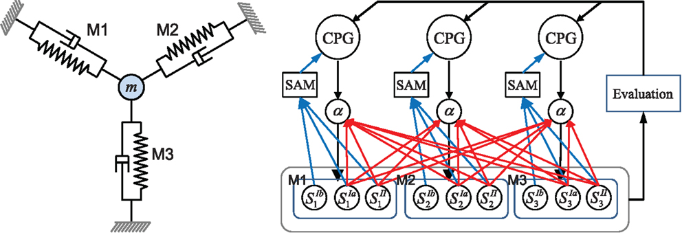
Figure 1. Left: the simple physics model used in some of the later investigations and right: the overall system architecture. A point mass is connected by three muscles (M1–M3) that are anchored at three equidistant positions. Each muscle is driven by an alpha motor neuron which integrates the descending command from the corresponding CPG neuron and the proprioceptive group Ia and II afferents (muscle spindles) from all muscles. CPGs also receive input from muscle spindles and are additionally fed by golgi tendon organ afferents (group Ib) providing muscle force information. Proprioceptive signals are integrated and modulated by a sensor adaptation module (SAM) before being sent to the CPG. An evaluation signal modulates the global bifurcation parameter of the CPGs, which drives the system between stable and chaotic regimes. The afferent weights (red arrows) of the alpha motor neurons are subject to adaptation which is guided by the evaluation signal. The architecture can be extended for a physical system of arbitrary degrees of freedom. See text for further details.

FIGURE 2

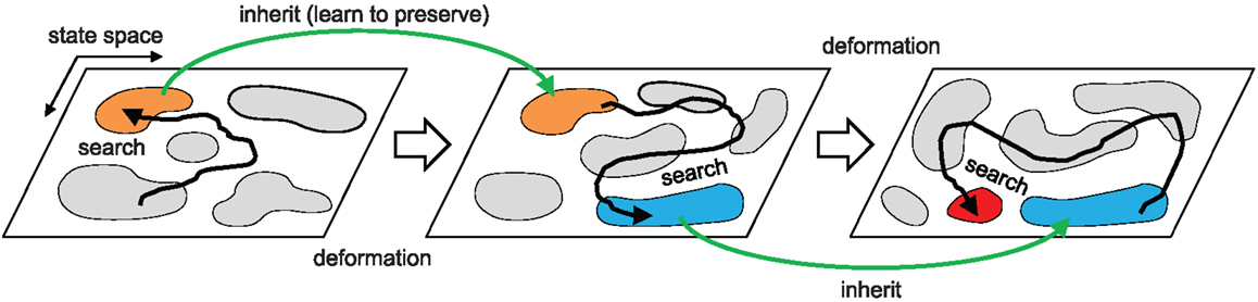
Figure 2. Overall search dynamics of the method. Chaotic exploration samples the population of attractors (motor patterns) that describe the intrinsic dynamics of the embodied system by driving the system orbit through the state space. The orbit is entrained in a high performing basin of attraction and the dynamics is further stabilized by proprioceptor adaptation. This process warps (mutates) the attractor landscape producing a new landscape that inherits major parts of the structure of the previous state space. The process repeats.

The method can be interpreted as an iterative, continuous, and deterministic version of stochastic trial-and-error search, which exploits the intrinsic chaotic behavior of the system. After describing the approach in more technical detail, we will demonstrate its application to two example embodied systems.

3.2. Central Pattern Generator and Adjustable Chaoticity of the Embodied System

Each alpha neuron is driven by the descending rhythmic signal generated from a corresponding CPG neuron (x^cpg), which receives only local sensory input from its corresponding muscle (Figure 1). A CPG neuron is modeled as an extended Fitzhugh–Nagumo [also known as Bonhöffer van der Pol (BVP)] oscillator (Fitzhugh, 1961; Nagumo et al., 1962), which was originally a simplification of the full Hodgkin Huxley spiking model (Hodgkin and Huxley, 1952), but its oscillatory membrane potential is often used for rhythm generation. A CPG neuron i operates according to the following coupled differential equations:

$\mathrm{\tau }{\dot{x}}_i^{\mathrm{cpg}}=c\left(x_i-\frac{x_i^3}{3}-y_i+z\right)+\mathrm{\delta }\left(I_i\left(s\right)-x_i\right)$ (1)

$\mathrm{\tau }{\dot{y}}_i^{\mathrm{cpg}}=\frac{1}{c}\left(x_i-b{y}_i+a\right)+\mathrm{\epsilon }{I}_i\left(s\right)$ (2)

$x_i=x_i^{\mathrm{cpg}}+x_T,y_i=y_i^{\mathrm{cpg}}+y_T$ (3)

where τ is a time constant, and a = 0.7, b = 0.675, c = 1.75 are the fixed parameters of the oscillator. The oscillator output is transformed by [x_T, y_T] = [−0.21387, 0.72019] in order to set the center of oscillation to the origin for further computational convenience. δ = 0.013 and ε = 0.022 are the coupling strengths for afferent input I(s) which is a function of the linear sum of proprioceptive sensor output s, processed by the sensor adaptation module (SAM) (Figure 1). I(s) can be viewed as integrated information from the interaction dynamics of the muscles, forming indirect couplings through physical embodiment (Kuniyoshi and Sangawa, 2006). z is the global control parameter for adjusting the chaoticity of the neuro-physical system. Asai et al. (2003a,b) demonstrated that changing one of the control parameters of two weakly coupled identical BVP oscillators (breaking symmetry) can produce various behaviors ranging from stable to chaotic dynamics. Our system can be regarded in this way by treating a CPG unit and the rest of the system (the physical system plus all other CPGs) as a pair of coupled oscillators. Just as with two standard coupled oscillators, a CPG sends information to the rest of system and receives information from it via I(s). In this way, every CPG views the rest of system as an identical BVP oscillator, treating the whole system as two scale-free coupled oscillators. Following Asai’s findings (Asai et al., 2003a), z is changed in the range [0.41, 0.73] allowing the neuromechanical system to exhibit stable limit cycles at z = 0.73 whereas z = 0.41 produces maximum chaoticity. All parameters values used were determined after preliminary experiments to find suitable values which enable the exploration capability of the system [for further details see Shim and Husbands (2012)].

For each CPG, the SAM performs homeostatic adaptation (Turrigiano and Nelson, 2004; Turrigiano, 2008) for sensor input by calibrating the raw sensor signal s from the corresponding muscle using a linear transformation, which continuously adjusts the amplitude and offset of the periodic sensor signal in order to emulate the CPG output. Since the z of the CPG is varied, the emulated input I(s) tries to mimic the waveform of the CPG at fixed z = 0.73 as in Asai’s two coupled BVP system. As outlined earlier, s is composed of group Ia and II type afferent signals together with input from a group Ib type signal, which is modeled as the normalized tension experienced by the muscle S^Ib = (k/k₀)((l − r)/r) (or its equivalent for rotational actuators). Observations from biology suggest that the Ib signal should be weighted more heavily than the other types (Conway et al., 1987; Pearson et al., 1992; Pearson, 2008). Hence, given raw sensor signal s, the adaptation function I(s) is:

$s=S^{\mathit{Ib}}+0.6\left(S^{\mathit{Ia}}+S^{\mathit{II}}\right)$ (4)

$I\left(s\right)=\left(s-\overline{s}\right)e^A+\left(\overline{s}+B\right)$ (5)

${\mathrm{\tau }}_h\dot{A}=\sqrt{p_{\mathrm{bvp}}}-\sqrt{\overline{{\left(I\left(s\right)-\overline{I\left(s\right)}\right)}^2}}$ (6)

${\mathrm{\tau }}_h\dot{B}=-\overline{I\left(s\right)}$ (7)

where $\overline{x}$ represents the low-pass filtered value of x as calculated from ${\mathrm{\tau }}_{h}d\overline{x}∕\mathit{dt}=-\overline{x}+x.$ The raw sensor signal s is linearly transformed by a multiplicative factor e^A and an additive factor B. A is updated by comparing the difference of the square root of the temporal average of the squares of the isolated BVP output (p_bvp ≈ 1.3932 at z = 0.73) and the transformed incoming signal I(s), which is analogous to the signal energy that reflects its strength or amplitude. B is updated by the offset deviation of I(s) from zero. The time scale of adaptation (τ_h) should be set longer than that of the oscillator, normally an order of magnitude larger. Again, all parameters values used were either taken from the literature or determined after preliminary experiments to find suitable values which enable the exploration capability of the system. The regulation of sensory activation achieved by this homeostatic mechanism not only ensures the systematic control of system chaoticity by the feedback signal, but also ensures that the neuro-mechanical system maintains a certain level of information exchange close to that of a weakly coupled oscillator pair so that their dynamics are regulated within an appropriate range to generate flexible yet correlated activities. This enables efficient chaotic exploration regardless of the physical properties of the robotic system and the type of sensors.

3.3. Performance Driven Feedback Bifurcation

The evaluation signal is determined by a ratio of the actual performance to the desired performance. The actual performance E can be any measurable value from the physical system. It can be defined as, for example, the forward speed of a robot, the power consumption of a mechanical system, or any hand-designed metric expressed as a function of physical variables of the system.

The time course of the bifurcation parameter μ ∈ (0, 1) is tied to the evaluation signal determined by the ratio of the actual performance to the desired performance, and it is used to control the CPG parameter z according to:

$z=0.73-0.\mathrm{32\mu }H\left(\mathrm{\mu }-\mathrm{ϵ}\right)$ (8)

${\mathrm{\tau }}_{\mathrm{\mu }}\dot{\mathrm{\mu }}=-\mathrm{\mu }+G\left(E∕E_d\right),G\left(x\right)=1∕\left(1+e^{16x-8}\right)$ (9)

${\mathrm{\tau }}_d{\dot{E}}_d=-E_d+E,{\mathrm{\tau }}_d={\mathrm{\tau }}_E\left(4H\left({\dot{E}}_d\right)+1\right)$ (10)

where τ_μ and τ_d are time constants and E_d is the desired performance. G(x) implements a decreasing sigmoid function which maps monotonically from (0, 1): maximally chaotic to (1, 0): stable regime. The heaviside function H(x) is used in order to ensure z does not fluctuate unnecessarily in the stable regime of the system by forcing the influence of the bifurcation parameter to zero when it is below a small threshold (μ < ϵ = 0.001). These two aspects ensure smooth stabilization. Since the method is intended for use in the most general case, where the robotic system is arbitrary, we do not have prior knowledge of what level of performance it can achieve. Using the concept of a goal setting strategy (Barlas and Yasarcan, 2006), the dynamics of the desired performance, E_d, are modeled as a temporal average of the actual performance, such that the expectation of a desired goal is influenced by the history of the actual performance experienced. This is captured in the “leaky integrator” equation for E_d above which encourages as high a performance as possible by dynamically varying E_d with rachet-like dynamics. The dynamics of the desired performance asymmetrically decays toward the actual performance by differentiating the decay rate τ_d, such that the rate of decrease is set five-fold lower than the rate of increase. The parameters values and form of functions used were determined after preliminary experiments to find suitable values.

Concrete examples of E are given later when we describe the embodied systems used in experiments with the method.

3.4. Weight Learning for Proprioceptive Afferents

The learning algorithm for the weights of the reflex circuit is based on the adaptive synchronization learning method of Doya and Yoshizawa (1992). Learning is activated at each epoch of the chaotically driven discovery process, once a motor pattern whose performance exceeds the current expectation has been found. This is similar to reward-modulated Hebbian, or exploratory Hebbian learning (Legenstein et al., 2010; Hoerzer et al., 2014). The change of weight w_ij of an alpha motor neuron i is given by:

$\frac{d{w}_{\mathit{ij}}}{\mathit{dt}}=\mathrm{\eta }\left\{\left({\mathrm{\alpha }}_i-\overline{{\mathrm{\alpha }}_i}\right)-{\displaystyle \sum _{k=1}^{2N}}{w}_{\mathit{ik}}\left(S_k-\overline{S_k}\right)\right\}\left(S_j-\overline{S_j}\right)$ (11)

${\mathrm{\tau }}_{\mathrm{\eta }}\frac{d\mathrm{\eta }}{\mathit{dt}}=-\mathrm{\eta }+H\left(\mathrm{ϵ}-\mathrm{\mu }\right)$ (12)

where α is the motor neuron output, S is a proprioceptive input (see the next section for details of how these are calculated), and $\overline{x}$ is the running average of x as calculated from ${\mathrm{\tau }}_{h}d\overline{x}∕\mathit{dt}=-\overline{x}+x,$ which is used to eliminate any bias effect from the offset of oscillatory signals so that learning is performed for phase synchronization between the alpha motor neuron and its afferent sum. The adaptive learning rate η smoothly activates reflex learning whenever the system enters the stable regime (when μ < ϵ = 0.001) by discovering a fit motor pattern. For the full derivation of the equation (11), see Shim and Husbands (2012).

4. Results and Analysis

The performance and properties of the new systems architecture were investigated with three simulated embodied models. In the first set of experiments, a minimal biomechanical model was used – the tractability of this model allowed detailed analysis, including visualizing the way the system’s state space changes throughout the search process. The second and third set of experiments involved a swimming robot learning to locomote and a legged robot learning to locomote, respectively; these systems were simulated using the ODE physics engine (Smith, 1998). These robot systems provide an indication of how the method translates to a more practical system involving more complex brain-body-environment interactions. The main focus of the results and analysis is on the simple biomechanical model as its tractability allows a more fundamental understanding of the method at work. The robot examples are intended more as illustrative case studies to demonstrate that the method can be applied to a variety of systems. Full analysis of these system is outside the scope of this paper and will be the subject of future work, but a sufficiently detailed analysis of the swimmer example is given to show that the method operates in a similar way to when applied to the simple biomechanical system.

4.1. Application to a Simple Biomechanical Model

A minimal physical system which is often used to model the dynamics of a compliant biomechanical system, at an abstract level, is a non-linear mass-spring network (Hill, 1938; Winters and Woo, 1990; Johnson et al., 2014). In this work, we chose a simple two dimensional system which has a single point mass driven by three simulated muscles which are modeled as spring-damper complexes (Figure 1, left). The system is chosen for its tractability and its abstract link to biological actuation, as well as its direct link to potential linear robot actuators. It has the basic elements of an (simulated) embodied system acting in the world through actuation and (proprioceptive) sensory feedback. The mathematical description of the dynamics of a mass connected by N muscles is:

$\dot{\mathbf{\text{x}}}=\mathbf{\text{v}}$ (13)

$\dot{\text{v}}=\frac{1}{m}{\displaystyle \sum _{i=1}^N}{F}_i+F_{\mathrm{e}}\left(t\right)$ (14)

$F_i=\left(-k_i\left(l_i-r_i\right)-c_i{\dot{l}}_i\right)e_i$ (15)

where x ∈ ℝ² and v ∈ ℝ² are the position and velocity of a point mass m. F _i represents the muscle force (with spring and damper constants k and c) exerted on the mass in the direction of e _i which is the unit vector in the direction of (x − p _i), where p _i is the position vector of the opposite end of the spring (of either another moving mass or a fixed anchor). l_i and ${\dot{l}}_i$ are the length and its derivative of the spring, and r_i is the rest length. F_e(t) is the external force (if it exists) acting on the mass.

A muscle is actuated by a simple yet biologically relevant model proposed by Ekeberg (1993), where the motor neuron output linearly controls a muscle spring constant (k_i). Each motor neuron output (α_i) consists of the corresponding CPG command signal $\left(x_i^{\mathrm{cpg}}\right)$ and the weighted sum of the proprioceptive inputs from the primary and secondary afferents of all muscle spindles, two per muscle (S^Ia and S^II), according to:

$k_i=k_{i0}+\tanh \left({\mathrm{\alpha }}_i\right)$ (16)

${\mathrm{\alpha }}_i=x_i^{\mathrm{cpg}}+g{\displaystyle \sum _{p=1}^{2N}}{w}_{\mathit{ip}}{S}_p$ (17)

$S_p=\left\{\begin{array}{ll}{S}_j^{\mathit{Ia}}=\mathit{sgn}\left({\dot{l}}_j\right)\sqrt{\left|{\dot{l}}_j\right|∕r_j},& \mathrm{if}p\mathrm{is}\mathrm{odd}\\ S_j^{\mathit{II}}=\left(l_j-r_j\right)∕r_j,& \mathrm{if}p\text{is even}& \end{array}\right.$ (18)

$j=\lceil \frac{p}{2}\rceil$ (19)

where g determines the contribution of proprioceptive input and k_i0 is the reference level of muscle stiffness. j indexes the muscles and p indexes the afferents (two per muscle, hence the use of the ceiling operator), N is the total number of muscles. The weights, representing peripheral feedback strengths, are the instantiation of the functional effect of spinal circuit plasticity. The approximation of the primary and secondary afferent from muscle spindles are modeled using muscle length and its stretching velocity. For the sake of simplicity, the primary afferents are modeled as the square root of muscle stretch velocity, and the secondary afferents are modeled using the muscle deformation from its resting length [similar to Marques et al. (2014)], both in units of muscle resting length. From the perspective of peripheral weight learning under periodic movements, as in this study, this allows a compact and convenient description of spindle afferents for dealing with phase relationship between CPGs, muscles, and peripheral sensors, because the sensor signals are decomposed into clearly distinguished phase components (90° phase shift between group Ia and II signals).

The fixed parameters for the mechanical model were set as: m = 1, k₀ = 1, c = 2, r_i = 1, and g = 0.1. The initial muscle length at the equilibrium position of the mass is 1. These values were chosen after preliminary experiments as they give a wide range of possible behaviors.

In our simple spring-mass system, the evaluation measure, E, is defined as a function of the phase relationship between CPG output signals, which is the theoretical analog of the locomotion performance of a robot as a function of interlimb phase relationships. The phase relationship of the three muscles used in this work can be expressed by two variables which are the phase differences between CPG 1 and 2 (φ₁₂), and between 1 and 3 (φ₁₃), which are updated at every moment when CPG 1 crosses its zero phase from 0₋ to 0₊. Thus the performance can be defined over a two dimensional manifold (on a torus, φ ∈ [−π, π]) by f :(φ₁₂, φ₁₃) ↦ E, which can be used to effectively visualize the system behavior on a 2D performance map. A simple performance landscape P can be defined by a mixed Gaussian functions on the surface of the 2-torus as follows:

$P={\displaystyle \sum _i}{m}_i{e}^{-\left(x_i^2+y_i^2\right)∕\left(2{\mathrm{\sigma }}_i^2\right)}$ (20)

$x_i=\min \left(\mathrm{2\pi }-|{\mathrm{\phi }}_{12}-x_{0i}|,|{\mathrm{\phi }}_{12}-x_{0i}|\right)$ (21)

$y_i=\min \left(\mathrm{2\pi }-|{\mathrm{\phi }}_{13}-y_{0i}|,|{\mathrm{\phi }}_{13}-y_{0i}|\right).$ (22)

For each individual Gaussian function i, (x_{0 i}, y_{0 i}) is the mean, m_i is the maximum, and ${\mathrm{\sigma }}_i^2$ is the variance. The actual performance E at any time instance is then given by leaky-integrating P over a short time scale in order to bias higher scores toward longer residence near that performance.

${\mathrm{\tau }}_e\dot{E}=-E+P$ (23)

See Figure 5 for the performance landscape, built from Gaussians, used in this study such that the system is required to perform non-trivial behavior (the highest peak, with height 1.0, is in the least stable region). Although abstract, this evaluation measure is very useful for a detailed analysis and visualization of how the system works, as will be shown later.

Both the quantitative analyses and qualitative observation of system behaviors were performed by numerical simulations of the above model. The time constants for the fast and slow dynamics were set based on the CPG period T ≈ 8.1 s. The rest of the parameters were set to: τ_e = τ_h = 5T, τ_d = 25T, and τ_μ = τ_η = T [based on previous experience these values were known to give good results (Shim and Husbands, 2012)]. Both the neural and physical simulations were integrated using the Runge-Kutta 4th order method with a step size of 0.001 s. The system is defined as “stable” or in the “stable regime” when the global bifurcation parameter is μ < 0.001 (as the parameter increases the system becomes more ‘unstable’) – all the CPG oscillations are gradually synchronized to have a certain phase relationship by indirect coupling through physical embodiment. Therefore, the entire neuromechanical system can be treated as a single autonomous dynamical system that consists of variables describing the dynamics of both the neural and physical parts. The same parameter values were used with the simulated robotic models described later (Section 4.5).

The following sections will mainly focus on the simple biomechanical model because its tractability allows detailed investigation and analysis giving useful insights into the properties of the overall approach. We first study how the initial unadapted system behaves from a dynamical systems perspective through which the system behaviors can be described and visualized in terms of the phase relationships of each oscillating degree of freedom. Various analyses are applied to describe the chaotic exploration process, followed by comparisons between the basic (no reflex learning) system and the system with reflex learning. The results are then extended to the locomotion of the simulated robotic systems, which includes interactions between the body and environmental forces.

4.2. Attractor Landscape of the Simple Biomechanical System

As each CPG is physically disconnected and is weakly excited only by its corresponding local afferent inputs, there is no significant deformation of the shape of the CPG limit cycle. The motion of the mass is driven by the damped spring muscles which are in turn driven by the corresponding CPGs, and the slow adaptive variables change passively due to these fast dynamics. Thus, as mentioned earlier, the behavior of our simple mass spring system can be represented by the phase relationships of the three CPG output signals at any time instance using two phase differences; i.e., based on CPG 1, the phase differences between CPG 1 and 2 (φ₁₂), and between CPG 1 and 3 (φ₁₃). This allows a particular coordinated motion of the neuromechanical system to be expressed on the two dimensional manifold of a 2-torus, where each axis on the surface represents the phase difference in the range [−π, π] (Figure 3). In this phase space, a particular synchronized oscillation of the system in a stable regime, after persisting for a sufficient duration, is shown as a point attractor whose neighbors converge to that point. The system in a stable regime can exhibit multi-period dynamics which is expressed as multiple points on the phase space. Other non-stationary dynamics in the system correspond to unstable regimes (or exploration regimes, where μ > 0.001) which can exhibit quasiperiodic dynamics expressed as a continuous line traces, and chaotic dynamics shown as scattered points (see Figure 3). In the space between the stable attractors in the stable regime of the system, there are various transient dynamics which the system undergoes before being entrained to the attractors. These transient states have different speeds of approach at different locations on the phase space, which represent the various stabilities of the transient phase relationships. Thus by representing the system like this, in terms of phase differences, it can be treated as a discrete dynamical system whose orbit is expressed as the time varying trace of a point on the phase space thus created.

FIGURE 3

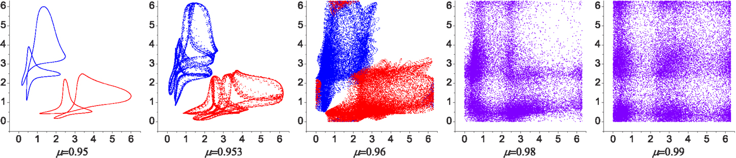
Figure 3. Poincaré maps for the phase evolution of the system with different chaoticities. The relative phases of CPG 2 and 3 were plotted [in the range (0, 2π) rad] when CPG 1 crosses zero phase. Over most of the range of the bifurcation parameter μ the system has two stable patterns (with small variations) as shown in the attractor landscape in Figure 5 (red region near B and C). Near the maximum value of μ the attractors start to lose their stability and are eventually merged into a chaotic dynamics. The two coexisting weakly chaotic attractors can be seen in some narrow region near μ = 0.96, which is reminiscent of the crisis-type route to chaos.

Figure 4 shows the numerically generated attractor landscape of the “basic” system in the stable regime where the reflex weights are homosynaptically set to 1, meaning each alpha motor neuron receives its proprioceptive afferents only from the corresponding muscle with a unit strength (w_ij = 1 if (j − 1)div2 = (i − 1) else w_ij = 0). Figure 4A is generated by plotting the phases of CPG 2 and 3 whenever CPG 1 completes its revolution. Independent simulations were started from uniformly spaced 20 × 20 inital points on the phase space with small random deviations (ξ = 0.01), each of which was run for more than 300 revolutions. The system has two stable point attractors at points (-2.87, 1.09) and (1.09, -2.87), which correspond to circular motions of the mass in opposite directions. The basins of these attractors occupy corresponding phase sub-spaces divided by unstable invariant sets, which are the heteroclinic connection between the unstable point (0, 0) and saddle point [≈(2.2, 2.2)]. The stability map of the phase space including other transient dynamics is visualized by color coded densities for each binned location (Figure 4B). As well as the two stable patterns, some relatively stable transient dynamics (i.e., dynamics which are relatively persistent, only changing slowly – which we refer to as “effective attractors”) are also regarded as candidate solutions for useful patterns. These slowly varying patterns can be easily captured and memorized by an external learning process (Shim and Husbands, 2012), because these patterns are sustained long enough to be used as the supervising signals for a learner.

FIGURE 4

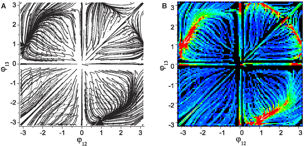
Figure 4. (A) Attractor landscape of the basic system in the stable regime where the reflex weights are homosynaptically set to 1. The diagram shows phase relationships between two different sets of CPGs for the simple biomechanical model. Each axis represents the phase difference between the outputs of CPGs 1–2 and 1–3. See text for further details. (B) Stability landscapes (2D histogram) for same: pixel colors represent the density of pattern appearance (visit duration). Colors are coded from blue (low density) to red (high), and black represents zero appearance due to the limited simulation time and the finite number of initial points.

The attractor landscape of the basic system reveals that a few groups of effective attractors are distributed symmetrically over the phase space. In order to perform a simple analysis of the statistics of the exploration behavior of system, we consider four different regions in phase space located in each quadrant, where the three quadrants (1st, 2nd, and 4th) have highly stable group of patterns (near the red points) and one quadrant (3rd) has patterns with the lowest stability. The total durations of the system orbit in each quadrant was counted for 400 runs as shown in the bar graph in Figure 5, which clearly shows how long the system stays within each quadrant. In order to perform chaotic exploration through performance driven bifurcation, the performance of each point on the phase space was defined by four gaussian hills [equations (20–22)], whose peaks are located at the specified mean locations in each quadrant (A–D). This performance map is designed such that the quadrant containing the most unstable pattern group (A) has the highest performance; thus, the goal of exploration is to visit and stay in the higher performing area as long (often) as possible despite of its low stability which counteracts the approach of the system orbit to that area. This makes the overall required behavior suitably challenging.

FIGURE 5

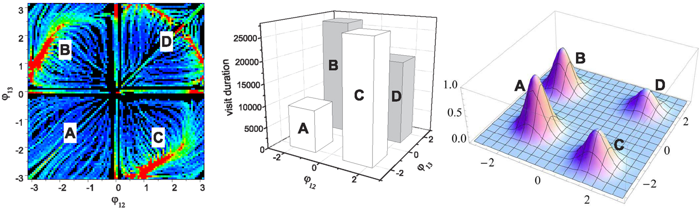
Figure 5. Assignment of performance on the initial (basic) landscape (leftmost). The performance map (rightmost) is generated by mixed Gaussian functions (of variance σ² = 0.4) whose mean positions are A:(-1.4, -1.3), B:(-1.9, 1.5), C:(1.5, -1.9), and D:(1.8, 1.8). The middle image shows the statistics of the visit durations in each of the four phase regions. The height of each bar is simply the total sum of the values at all points in each quadrant of the basic landscape, which represents the average stability of the corresponding quadrant. Note this is not the result of chaotic search, but it is just a simplified quantification of the basic landscape shown in Figure 4. These four bars effectively describe how long and how often the system orbit stays around each of the four search positions defined by the performance map (A,B,C,D) when chaotic exploration is enabled. The performance map was defined such that the pattern in the least stable region A has the highest score (peak value of 1.0). The other three peak performances were set to: B = 0.8, C = 0.6, D = 0.4.

4.3. Driving the System Orbit through Adaptive Bifurcation

The stable dynamics of the system begins to fluctuate as the global bifurcation parameter μ increases, exhibiting a series of dynamics from quasiperiodicity to chaos (Figure 3). While two coupled BVP oscillators always exhibit non-stationary dynamics for the entire positive range of μ > 0, the embodimentally coupled neuromechanical systems shows stronger synchronization of CPGs, such that over most of the range of the bifurcation parameter μ, two stable patterns are evident (with a small variations), as in the stable regime (stable behaviors as in Figure 4). Near the maximum value of μ each of the stable attractors start to lose their stability and exhibit a series of non-stationary dynamics from quasiperiodic to chaos until they are eventually merged to create a single chaotic dynamics, which relates to the crisis-type route to chaos. In the higher chaotic regime, the complex transitory dynamics drives the system such that it briskly wanders around phase space: thus providing the mechanism powering exploration.

During exploration, the bifurcation parameter is controlled by the performance evaluation according to equations (8–10), which continuously drives the system between stable and chaotic regimes. Figure 6 shows a visualization of a couple of example epochs of chaotic search by feedback driven bifurcation. The continuous exploration behavior of the system is clearly seen as a series of jumps from one phase region to another according to the ratio of the actual to desired evaluation signals. When the actual performance becomes higher than the desired performance within a small tolerance ϵ, the system is regarded as having discovered a pattern and it stabilizes the orbit by setting the control parameter μ to zero. If the discovered pattern is stable, the system yields a stationary state without further exploration, where the ratio of actual performance to desired performance balances at slightly above unity with a small sub-tolerant fluctuation (Shim and Husbands, 2010; Shim and Husbands, 2012). However, in order to investigate the statistics of the long term behavior of the exploration process, the performance map is designed such that the stable patterns do not have high performance, making it extremely hard for the system to settle in a stationary state, forcing it to continuously explore and visit the four transient patterns (Figure 5). Thus, after the system enters the stable regime by visiting a transient pattern, the performance will gradually decrease as the system orbit drifts away from the pattern; this triggers the resumption of exploration (making the system leave the stable regime) by the destabilization of the system through changes to μ.

FIGURE 6

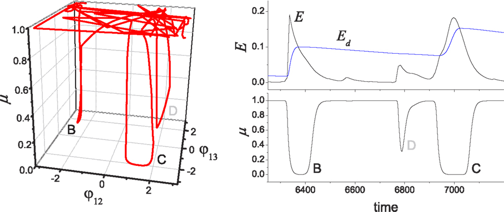
Figure 6. Chaotic jump between attractors. (Left) An example of chaotic exploration is shown in (φ₁₂, φ₁₃, μ) space, and (right) the time course of performance (E) and desired performance (E_d) is shown with the global bifurcation parameter (μ). The system orbit jumps from the stable regimes near pattern B to pattern C, where the complete approach to be near pattern D failed due to the insufficient level of E/E_d.

By running the chaotic exploration for a sufficient amount of time, an analysis was generated of how the basic system explores and becomes entrained to each group of patterns, as illustrated in Figures 7A–C. The simulation was run for more than 1.2 × 10⁵ oscillation periods and the visits of the system to each quadrant was counted, which represents the visits to the regions occupied by each pattern. The visited locations on the phase space in the stable regime shows that feedback driven exploration found a variety of transient patterns wherever a reasonable density of patterns exists. Since the slow dynamics of the desired performance E_d decays asymmetrically (rate of decrease is lower than rate of increase), the system is biased toward the higher performing patterns. The exploration bias is also influenced by the stability of patterns and the relative differences of their performances. The exploration process’s visit duration in each region (Figure 7B) shows that the duration in region A (which has the highest performances) exceeded that of pattern D despite its low stability (as in Figure 5 middle), although the two most stable patterns (patterns B and C) still dominate the total residence time. However, the visit frequencies (count) regardless of the duration of each visit (Figure 7C) reveal that the pattern A is most frequently visited followed by patterns B–D, which is the exact order of their performance level. These results demonstrate that the chaotic exploration process acts as intended with the new architecture. The next section describes the improved exploration process produced by incorporating reflex learning into an iterative version of the method. Here the system not only visits and stays longer in the higher performing patterns, but also enables visits to a wider variety of patterns by adaptively deforming the stability landscape of phase space.

FIGURE 7

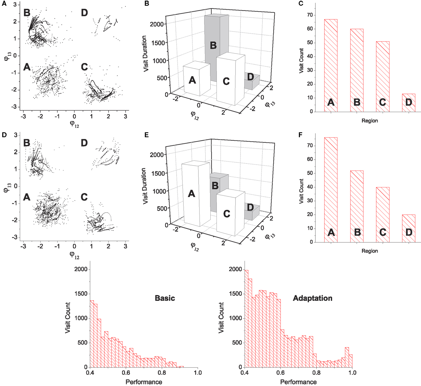
Figure 7. Statistics of pattern search by chaotic exploration without (A–C) and with (D–F) reflex learning (both simulations are run for 12,000 CPG periods). (A,D) Visited points are plotted on the phase space whenever the system is in the stable regime (i.e., when the global bifurcation parameter is μ < 0.001). (B,E) Total visit durations near each pattern in units of CPG revolution, i.e., the number of points in each quadrant in (A,D). (C,F) The number of visits to each region. Visiting events are counted only when the system entered into the stable regime from the exploration regime (increase count whenever μ falls below 0.001). (Bottom row) Histograms of visit count vs performance. The appearance of performance values are calculated using a bin size of 0.2.

4.4. Exploration with Reflex Learning

To address the effect of reflex learning, we first investigate how the attractor landscape of the simple biomechanical embodied system is deformed by changing the weight strengths of proprioceptive afferents. Starting from the attractor landscape of the basic system (unit weights), a pattern is selected by either manually stabilizing the transient dynamics or choosing one of the stable dynamics by spontaneous entrainment. After the system is stabilized, the phase locked oscillations between alpha motor neurons and muscle sensors are used as the target pattern for the reflex learning, which tries to maintain the selected coordinated dynamics. The fixation of system is achieved by disconnecting all sensor inputs to CPGs, so that the phase differences between CPGs are anchored without further drift. This forcibly stabilizes the movement of the entire neuromechanical system, hence fixing the phase relationship between the alpha motor neurons and muscle sensors. Reflex learning is enabled as in equation (11), and is run until either all weights are converged or a certain time limit is reached. Using the newly obtained reflex weights, the inputs to CPGs are re-enabled (in case of manual fixation), and the new (deformed) attractor landscape is generated by the same method as in Figure 4. This procedure is repeated to generate a sequence of landscapes as shown in Figure 8.

FIGURE 8

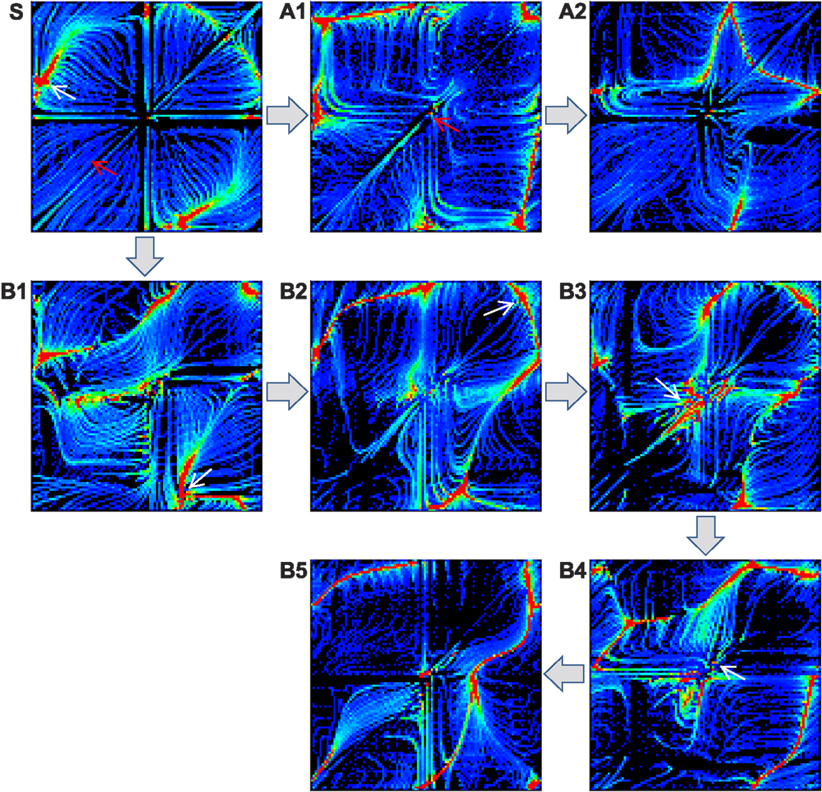
Figure 8. Deformation of attractor landscape by reflex learning. Starting from the basic system (S), the reflex circuit is learnt (until the full convergence of weights) for the selected patterns (which are indicated by red and white arrows) on the current landscape to generate a deformed landscape. This procedure (select-learn-deform) is repeated for the consecutive landscapes. Except the red arrow on S (intentionally fixed to the highest performing pattern), only the stable patterns were selected on the corresponding landscapes, i.e., one of the red colored regions which is found by running the system for sufficient duration. Two example sequences of landscape deformations are shown: S-A1-A2 (indicated by patterns with red arrows) and S-B1-B2-B3-B4-B5 (white arrows).

The figure shows two different sequences starting from two initally selected patterns (indicated by arrows in Figure 8S), one is from a stable pattern by spontaneous entrainment (white arrow) and the other is from a manually fixed transient pattern (red arrow). The first sequence (A1–A2) was started from the highest performing pattern (pattern A in Figure 5, manually selected) in order to see whether the deformation of the landscape is positively influenced by the selection of the desired pattern, whereas the second sequence (B1–B5) was started from a randomly entrained stable pattern. The experiment shows that learning for a specific unstable pattern has little immediate effect on increase in stability of the region near that pattern. Even if we know in advance the location of a high performing attractor, forcibly applying reflex learning directly toward that attractor gives us little immediate help in stabilizing the region near that attractor if its location is unstable. Rather, a more promising way to reach the unstable high performing region is to follow a less direct “natural path” by learning for naturally emerging attractors which are stable. The latter sequence (B1 to B3) is of this kind, because it involves learning for sub-optimal but naturally selected patterns resulted in more stabilization of the desired region as the state space is gradually changed by the learning process. Both learning sequences show that the reflex learning creates/deforms the stable regions (attractor basins) while it generally preserves the regions near the previously selected patterns if the previous pattern is stable enough. This shows that over the course of landscape deformation by learning, the more stable regions survive longer in the consecutive landscapes, there being more chance of discovery of similar patterns near that region by the exploration process. Therefore, the exploration-learning procedure also promotes the search of patterns which have better stability and higher performance, naturally opening up new, sometimes circuitous, routes to higher performance regions. Hence the reflex learning process can be thought of as a kind of replication with variation of the whole phase space with a bias toward preserving both the more stable and fitter regions. As will be discussed later, this means that the dynamics of the overall iterated exploration-learning process begins to have much in common with evolutionary search.

During exploration, reflex learning is adaptively enabled by equation (12). Whenever the system enters a stable regime by pattern discovery, the reflex weights are learnt so as to achieve the synchronization of alpha motor activity and proprioceptive input signals – a process which tries to sustain the currently discovered pattern. If the visited pattern is transient, the system returns to the exploration regime due to the degeneration of the evaluation signal, and the learning is disabled. Exploration is resumed on the new landscape modified by the previously learnt reflex circuit. Since the performance map was previously defined such that the system only visits transient patterns, the system with reflex learning also continuously alternates between the stable regime and exploration regime, and the statistics of long term exploration behavior were analyzed for this version of the system. Figure 7 shows the comparison of the exploration processes without (A–C) and with (D–F) reflex learning. The visit duration statistics show that the system with reflex learning stays longer in the desired region (higher performing but initially having low stability), which means that the system orbit has overcome the instability of the desired patterns by actively changing the attractor landscape of the phase space by learning. By the adaptive deformation of the attractor landscape, the system is able to visit new patterns which were hard, or even impossible, to reach in the previous landscape. The deformation of the attractor landscape can be interpreted as the creation of new attractors and the destruction of existing ones, driven by chaotic dynamics.

Both systems show that the visit count of the desired region A is the highest among the four regions due to the exploration bias toward higher performance. Higher performing patterns tend to be more visited because of the use of slowly decaying desired performance (E_d, the performance threshold in order to enter the stable regime). For example, if E_d goes higher than 0.8 (peak score of region B) due to the previous discovery of the pattern in region A (peak score 1.0), approaching only the patterns in region A, whose performance is higher than 0.8, can stabilize the system until E_d falls lower than 0.8. Thus, only the patterns whose performances are higher than the current value of E_d have a chance to be visited, which gives a higher probability to the visit of higher performing patterns. Given the total simulation time for both system, the system with learning stays longer at each visit than the basic system, so its total visit count within a specified simulation duration is lower. Nonetheless, the visit counts figures show that the system with learning still visited region A more often than the basic system. The performance histograms also show that exploration with learning visited the highest performing patterns (E ≳ 0.9) which could not be accessed at all by the basic system. This indicates that the learning system can explore a wider variety of patterns with greater stability by employing adaptive landscape deformation.

Figure 9 shows color coded plots which allow us to visualize the performance levels of the visited patterns of the basic (A–C) and learning (D–F) system. The residence of the system in each region (A, D) shows that the system with learning has a greater density of points in the highest performing region (3rd quadrant). Studying the visited points with maximum performance in each visit (C, F) also shows that the system with reflex learning discovered higher performing patterns than those that could be reached by the basic system.

FIGURE 9

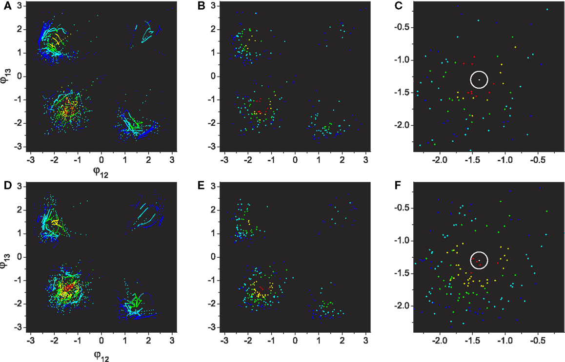
Figure 9. Performances of visited regions through exploration. (A–C): Basic system. (D–F): System with adaptation. All plot points are color coded by their performance from blue to red (0.0 ≤ E ≤ 1.0, increase step of 0.2). (A,D) The same plots as Figure 7 except the points are colored by their performance levels. (B,E) Plots depicting only the points of maximum performances within each visit. (C,F) Magnification of the 3rd quadrant (lower left) of (B,E), which contains the highest performing patterns. The center of the white circle is the highest performance (E = 1.0) defined in the phase space.

Together these results demonstrate the power of the integrated use of the two adaptive processes (chaotic exploration, reflex learning) to iteratively deform the state space toward the most amenable dynamics for finding and persisting with high performance behavior.

4.5. Experiments with Simulated Robotic Systems

The results described above were extended to the generation of locomotion behavior in two simulated robotic systems in order to see the effect of exploration with reflex learning in a more practical situation which addresses embodied behavior through neuro-body-environmental interaction. Robotic systems with and without reflex learning were both able to readily find high performing patterns that provided efficient locomotion motion through appropriate coordination of limbs. However, the system with learning found higher performance patterns in both cases. In both cases, the required behavior was to move straight ahead in an efficient manner. The simulated robots used are shown in Figure 10. The parameters for the exploration and learning systems were identical in each of the three applications, demonstrating the generality of the method.

FIGURE 10

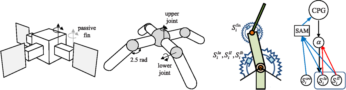
Figure 10. Robot simulation models. The three finned 2D swimmer has thin rigid fins at the end of each arm which are attached by a passive torsional spring. The quadruped has four legs attached to a spherically shaped torso, and the limbs are joined by upper and lower joints for horizontal and vertical leg movements. A torsional muscle is attached at a virtual frame on the parental limb in order to facilitate the movement of the joint angle within a specified range, up to where the stretched angle of two antagonistic torsional muscles at the neutral position of the joint becomes double the rest angle. The swimmer uses fin angles, S^fin for CPG sensor input (S^CPG), whereas the quadruped uses muscle force sensors S^Ib.

4.5.1. Swimming robot

The swimming robot used for locomotion studies is shown in Figure 10. The three fins are used for locomotion in a simulated underwater environment. The swimmer was constructed using a 3D rigid body simulator, but it was constrained to move only on the x–y plane, so that it effectively undergoes 2D dynamics. Each fin of the 2D swimmer was modeled as a non-linear damped torsional spring, which is subject to simulated hydrodynamics (Shim and Kim, 2006). Each arm is driven by a pair of antagonistic torsional muscles which is the angular version of the mass-spring system described earlier, so the system has a total of six CPG-muscle units. Proprioceptive information is similar to that for the linear muscles of the previous model, except using angular velocity and displacement, and the muscle force information from the group Ib afferent was replaced by the bending angle of the (passive) fin which represents the hydrodynamic force exerted on the fin surface. This latter quantity is fed, with opposite signs, to the sensor adaptation modules of the corresponding pair of CPGs. This reflects the interactions between arm movements and the hydrodynamic environment. Because the fins are passive, their interactions with hydrodynamic forces as they are driven indirectly by the limbs, results in subtle, complex dynamics which, coupled with the fact that there are an odd number of limbs, makes the task more challenging than it might at first appear.

To produce the desired locomotion behavior, the evaluation measure for the robot was based on its forward speed. Since the system has no prior knowledge of the body morphology of the robot, it does not have direct access to the direction of movement or information on body orientation. In order to facilitate steady movement in one direction without gyrating in a small radius, the center of mass velocity of the robot was continuously averaged over a small time window, and its magnitude was used as the performance of the system. The performance signal E at any time instance was calculated by applying a leaky integrator equation to the velocity vector, v, as follows:

$E\left(t\right)=\left|\right|\overline{\text{v}}\left|\right|,$ (24)

${\mathrm{\tau }}_E\frac{d\overline{\text{v}}}{\mathit{dt}}=-\overline{\text{v}}+\text{v}.$ (25)

The time scale of integration was set as τ_E = 5T where T is the period of an oscillator, the neural system parameters were the same as for the simple biomechanical model, other robot model parameters are given in the Supplementary Material; for further details of this robot model, see Shim and Husbands (2012).

Figures 11–15 give insight into the behaviors developed and the performance of the method in this application. Figures 13 and 14 illustrate high and medium performing behaviors respectively. E > 0.6 indicates a high performing locomotion behavior, E < 0.2 is a very poor one and in between values medium performance.

FIGURE 11

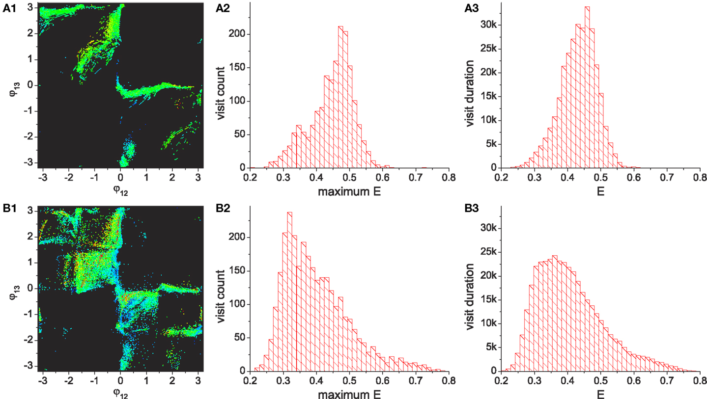
Figure 11. Chaotic exploration of 3-fin swimmer [(A1–A3): Basic system. (B1–B3): System with reflex learning). (A1,B1) are the phase difference plots of three limb movements which are chosen as the representative behaviors of the system driven by six CPGs. Whenever the system stabilizes to a pattern, the phase difference between limb 1–2 and 1–3 were plotted using colors representing their performance [from blue to red: 0.2 ≤ E ≤ 0.6, black if E < 0.2 (very poor performance), red if high performing (E > 0.6)]. (A2,A3) and (B2,B3) are histograms representing the visit count and duration for each performance bin. The visit count histogram is produced for the maximum performance reached at each visit span.

FIGURE 12

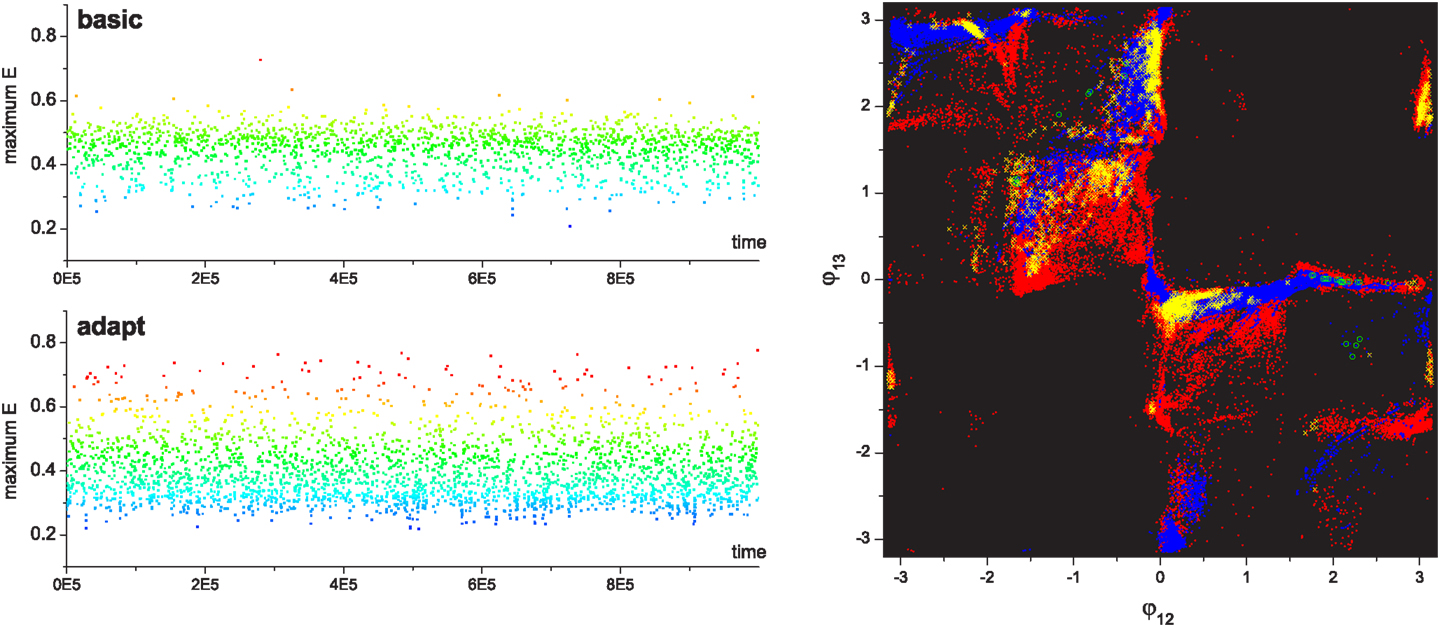
Figure 12. [Left] Time course of max performance at each visit in finned swimmer exploration. Plots are color coded as in Figure 11. [Right] Superposed image of phase difference plots from Figures 11A1,B1. Visited points of the basic system (blue) is shown over the system with adaptation (red), and the points whose performances are higher than 0.6 are shown as cyan circles (basic) and yellow crosses (adaptation). It can be seen that a large part of the high performing behaviors produced by reflex learning are located near the edge of areas of basic behaviors, indicating that a small difference in limb phase relationships made by adaptation can result in large performance differences, indicating a rugged fitness landscape.

FIGURE 13

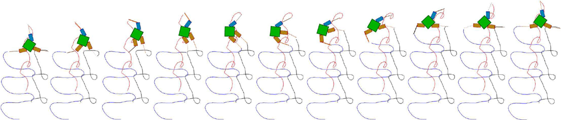
Figure 13. Snapshots of a high performing three fin swimmer locomotion showing fin tip trajectories (E = 0.81). The snapshots are laid out left to right showing a sequence where the robot is swimming upwards in a trajectory which is very close to a straight line. Color coded fin tip traces (one color for each fin) are shown trailing the robot, indicating the regular, but fairly complex motion, of the fins.

FIGURE 14

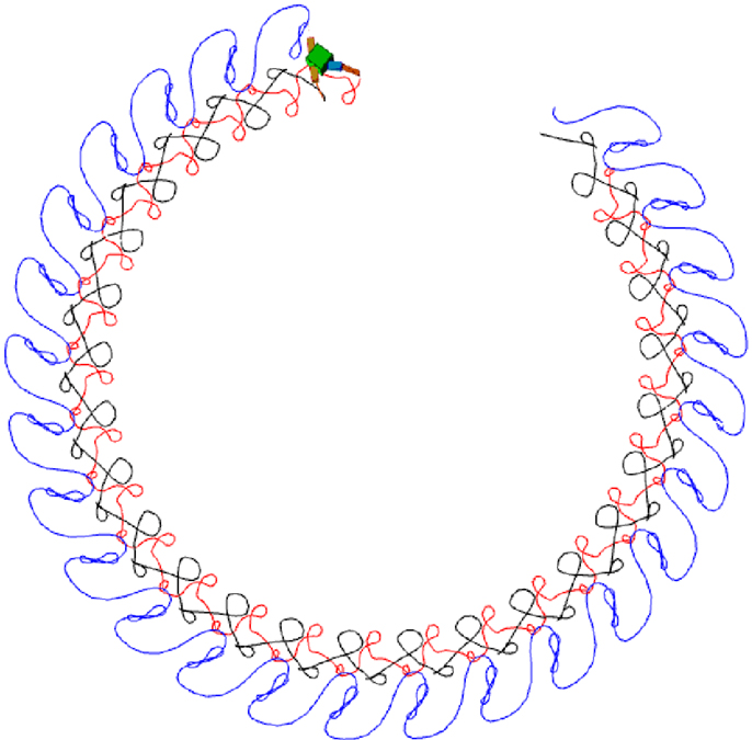
Figure 14. Snapshots, a less well performing circular locomotion (E = 0.5), performed by a swimming robot. The figure shows a sequence of color coded fin tip movements (as in Figure 13) indicating the circular path taken by the robot (which does not score as well as straight line motion). Again it can be seen that the fins make regular, repeated, fairly complex movements.

FIGURE 15

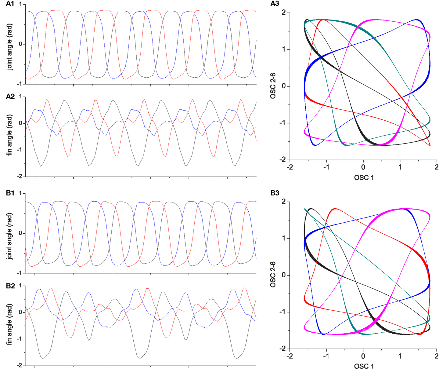
Figure 15. Two locomotor behaviors of the three finned swimmer. (A1–A3) shows an example of high performing locomotion (E ≈ 0.8, the behavior shown in Figure 13); (A1): Joint angles, (A2): Passive fin angles, and (A3): The output of CPG oscillators 2–6 vs. oscillator 1. (B1–B3) describe one of the less well performing behaviors [E ≈ 0.5, the behavior shown in Figure 14 which is a similar motion to that in Figure 13 but moving on a circle (lower performance than straight motion)]. Even if the interlimb coordination in (B1) is similar to (A1), the slight deviations in the phase relationship and amplitude from (A1) results in significant differences in fin bending due to the non-linear interaction of body and fluid forces [see differences between (A2) and (B2)]. More visible differences can be seen between the oscillator output trajectories (A3,B3).

Analysis of statistics for the exploration of robot locomotor patterns is shown in Figure 11. Since the robotic system has six CPG modules whose phase patterns cannot be visualized on the 2D phase space, the phase differences between movements of the three arms were used to represent the behavior of system. It is clearly shown that the robot with reflex learning visited a wider variety of patterns and found higher performing patterns than the basic system. Interestingly, the histograms for the performances of visited patterns shows that the performances of the most frequently visited patterns are around 0.5 in the basic system, whereas the system with learning most frequently visited patterns whose performances are around 0.3. It can be inferred that in this case a sizeable proportion of the newly visited patterns created by reflex learning have a lower performances, but even so a significant portion of them have higher performances than exist in the basic system. This also can be seen in the time course of the performances of visited patterns (Figure 12). The far denser band of red dots (high performing patterns) on the bottom left time course clearly demonstrates the efficacy of the method with reflex learning. This point is also reinforced in the phase differences plot at the right of the figure where we can see far more, and far more widely spread, high performing points resulting from the method with adaptation (reflex learning) turned on. It can be seen from these two figures that the system with learning discovered not only more higher performing patterns, but also far more lower performing ones than the basic system. We can understand this by considering that in contrast to the smoothly distributed performances of the simple mass-spring model, the performance space of the robotic system is highly rugged. This is because a small deviation of phase relationships from some high performing locomotion pattern can suddenly destroy ongoing behavior, especially in the case of underwater or aerodynamic locomotion where the robot must deal with stalling effect (as in the example here). As the reflex learning process deforms the state space, creating new attractors, because of the ruggedness of the landscape, many of these will be of lower fitness – however, they still open up new pathways to higher performing patterns as can be seen here in the case of the swimming robot. This tells us that the method performs well in complex, rugged fitness landscapes.

Figures 13 and 14 show, respectively, typical high and medium performing behaviors. It can be seen that the method readily develops regular motor patterns that allow smooth movement through the simulated fluid. Figure 15 illustrates the oscillatory motions underlying these behaviors. The CPG output plots at the right of the figure show both how stable dynamics have been developed, and how small changes in the relationships between the oscillators result in subtle changes to the arm and fin motions (as indicated in the time course plots to the left of the figure) which in turn result in significant changes in overall behavior. Such changes are effectively explored and exploited by the method.

4.6. Walking Robot

In order to further demonstrate the generality of the method, it was also applied to a legged robot as shown in Figure 10. A simulated quadruped robot with two actuators per leg (requiring 4 CPG oscillators per leg) was used and the required behavior was forward locomotion across a flat plane. The same framework was used as in the previous two examples, with the number of actuators now 8, each driven by a pair of antagonistic “muscles,” resulting in 16 CPG oscillators. Parameter values were the same as in the swimming robot example and the same performance formulation of the performance measure, E, was used [equation (24)].

A typical good behavior developed by the method (with reflex learning) is shown in Figure 16. The simple quadruped, with a spherical body, is illustrated at the top of the figure in a series of snapshots as it walks in a straight line left to right. Details of the physical parameters used for the simulated robot are given in the Supplementary Material. The time course plots of joint angles and muscle forces, and the oscillator output plots, show that the method has again readily developed stable motor patterns that allow the coordination of the legs to generate efficient walking. Many of the discovered legged motions included some foot slippage, which is energy-inefficient if too great. However, an interesting and unexpected discovery was that the method found particular combinations of different foot slips and asymmetric limb movements resulting in close to straight locomotion of the whole body (as an alternative to bilaterally symmetric gaits).

FIGURE 16

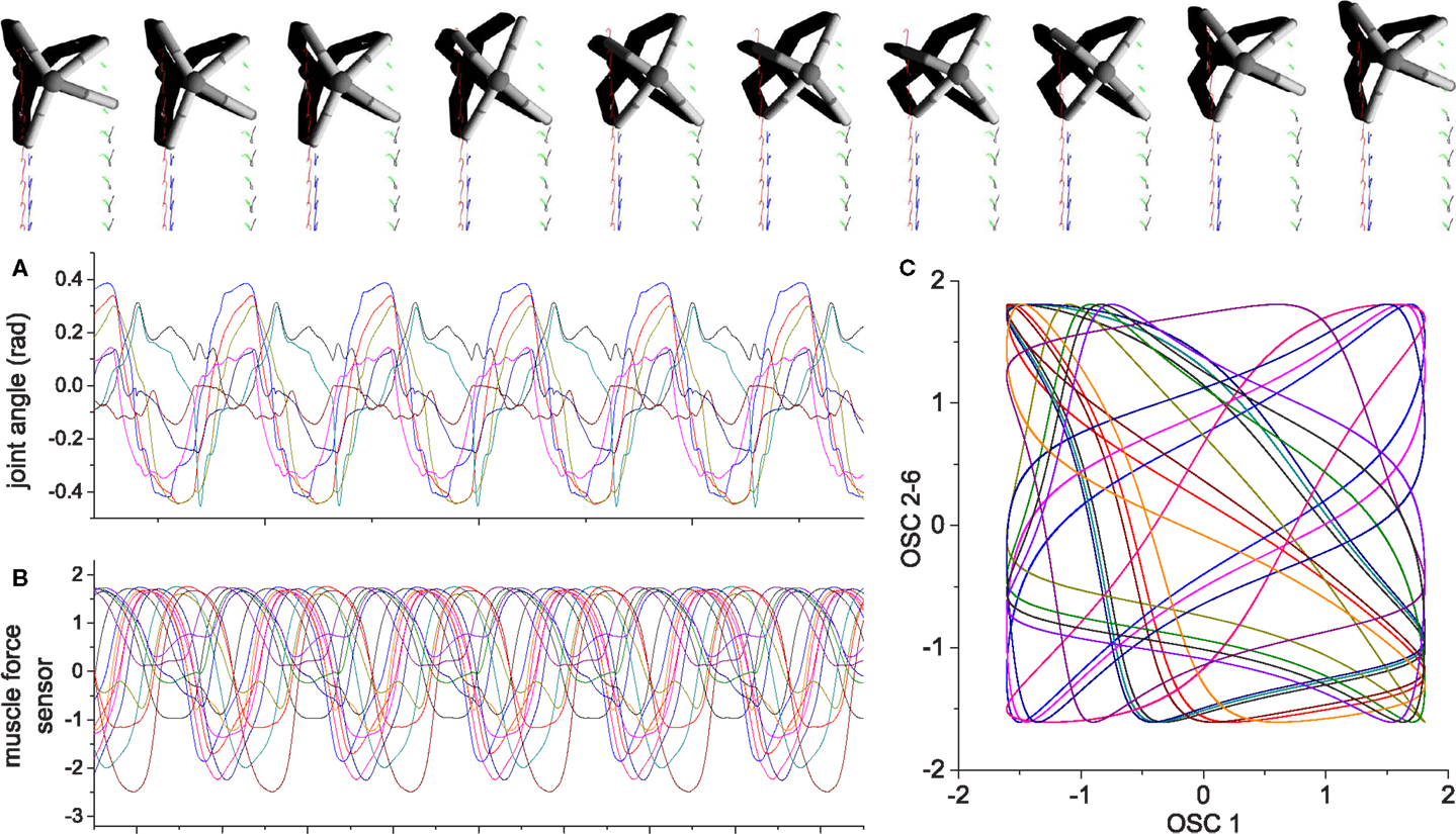
Figure 16. An example of quadruped locomotion. Colored traces in the snapshot images represent the foot contact trajectories of each leg. (A,B) are time plots of the 8 joint angles and 16 muscle force sensors, (C) depicts the output of oscillators 2–16 vs. oscillator 1. The parameters of the physical model are given in the Supplementary Material. Muscle force is calculated in the same way same as the previous examples, except the signal is low-pass filtered (by a leaky-integrator equation) with time constant τ = 0.25 in order to prevent strong jerky signals from muscle sensors at the time of stance-to-swing transition (because of simulated Coulomb friction).

It is outside the scope of this paper to analyze this walking example in greater depth; it is given as a simple illustrative case study to make clear the generality of the method. The same general framework, and set of parameters, has been successfully applied to three quite different examples.

5. Discussion

The results in the previous section demonstrate the power of the integrated use of the two adaptive processes (chaotic exploration, reflex learning) to iteratively deform the state space toward the most amenable dynamics for finding stable high performance behavior. The iterative approach was shown to be more powerful than a basic non-iterative approach with new paths to higher fitness attractors being opened up by the more sophisticated method.

Creation does not emerge from a zero-base but is stacked on previous habits and experiences, and the loose channel of information flow for this creative process is structured by body-environmental constraints. Our system implements continuous and fully dynamic exploration-learning-self-tuning sequences where the previous learning experience creates new routes to undiscovered regions in the search space which could not be reached in past explorations. Chaos sensitizes the system to leave currently habituated (motor) patterns and enables exploration of new patterns within the landscape of patterns which are self-organized by the given physical embodiment. The shape of the landscape is defined by the stability of self-organized patterns and the system orbit is entrained in one of the basins of attraction by chaotic exploration with adaptive bifurcation.

While the chaotic nature of the oscillator dynamics (depending on the z parameter) is well established in the literature (Asai et al., 2003a) and the chaotic regime of the simple biomechanical system is demonstrated by the classic scattered points of the Poincaré map of the phase evolution of the system (Figure 3), quantifying the chaotic nature of the overall dynamics of the simulated robotic systems is more involved. This requires fairly complex sets of calculations based around Lyapunov analysis (Wolf et al., 1985; Rosenstein et al., 1993). The amount of space required to explain and present the calculations puts such an analysis outside the scope of this paper. However, an analysis, for simulated robots very similar to the ones used in this paper, is given in Shim (2013) demonstrating the chaotic nature of their dynamics during the exploration phase.

The overall process has a number of interesting parallels with evolutionary dynamics. The whole system (literally) embodies a population of (motor behavior) attractors, which are sampled by chaotic exploration. The propriocetor learning process warps (mutates) the state space such that a new landscape of attractors is created, but one that inherits the major properties of the previous (ancestor) landscape (replication with variation). The process repeats with the new population being sampled by chaotic exploration. The overall search dynamics are vividly illustrated in Figure 8. The evaluation mechanism effectively selects a sufficiently fit attractor which then directly influences the creation of the new landscape through application of the proprioceptor adaptation mechanism. The dynamics of E_d, the desired performance level, controlled by τ_d [equation (10)], is analogous to selection pressure. The current form of the system is like an ultra elitist evolutionary algorithm: only a single fit member of the population directly influences the next generation, other members only having an indirect effect through influencing the way the population is sampled by chaotic search. An interesting extension, and the focus of further work, will be to incorporate (fitness dependent) influence from a larger sample of the population in creating the new attractor landscape. This will then create solidly Darwinian neurodynamics in a neural architecture that is both practical and fully biologically plausible. This work thus points toward possible fully integrated and intrinsic mechanisms, based entirely on neuro-body-environment interaction dynamics, that might be involved in creating Darwinian processes that could continually run within the nervous systems of future robots (Fernando et al., 2012) without the need for off-line processing or sleight-of-hand magic black boxes.

Since the population of attractors is effectively implicit – the intrinsic dynamics of the system drive it to sample the space of attractors – our embodied system can be thought of as a kind of generative search process. The overall brain-body-environment system (literally) embodies a population of motor pattern attractors through its dynamics; it cannot help but sample them during the exploration phases. This is loosely analogous to the generative statistical models used by estimation of distribution algorithms (EDAs) (Pelikan et al., 2000, Larraaga and Lozano, 2002), which are well established as part of the evolutionary computing canon. Instead of using an explicit population of solutions and the traditional machinery of evolutionary algorithms, EDAs employ a (often Bayesian) probabilistic model of the distribution of solutions which can be sampled by generating possible solutions from it. Search proceeds through a series of incremental updates of the probabilistic model guided by feedback from sampled fitness. In an analogous way, our generative system (the overall system dynamics) is incrementally updated in relation to evaluation based feedback. The overall system dynamics is the generative model, the exploration phase is the sampling step, with E_d controlling a selection pressure, and the reflex learning process provides a kind of mutation which facilitates the replication (with variation) of the whole phase space, now containing a slightly different population of attractors but with a bias toward preserving more stable and fitter areas of phase space.

The results illustrated in Figures 8–16 demonstrate a powerful and general mechanism that can be applied without prior knowledge of the embodied morphology or environment. Future work will apply the method to a range of simulated and real robots and demonstrate its ability to re-adapt in the face of change and cope with noise, as well as further exploring its role in explaining aspects of biological adaptation.

6. Author Contributions

Concept and design of experiments: YS and PH, implementation, running experiments, and analysis: YS, writing paper: YS and PH.

Conflict of Interest Statement

The authors declare that the research was conducted in the absence of any commercial or financial relationships that could be construed as a potential conflict of interest.

Acknowledgments

We acknowledge useful discussions with members of the CCNR and the INSIGHT consortium. Funding: This work was funded as part of the EU ICT FET FP7 project INSIGHT.

Supplementary Material

The Supplementary Material for this article can be found online at https://www.frontiersin.org/article/10.3389/frobt.2015.00007

References

Aida, T., and Davis, P. (1994). Oscillation mode selection using bifurcation of chaotic mode transitions in a nonlinear ring resonator. IEEE Trans. Quant. Electron. 30, 2986–2997. doi: 10.1109/3.362706

CrossRef Full Text | Google Scholar

Akazawa, K., Aldridge, J. W., Steeves, J. D., and Stein, R. B. (1982). Modulation of stretch reflexes during locomotion in the mesencephalic cat. J. Physiol. 329, 553–567. doi:10.1113/jphysiol.1982.sp014319

Pubmed Abstract | Pubmed Full Text | CrossRef Full Text | Google Scholar

Asai, Y., Nomura, T., Abe, K., and Sato, S. (2003a). Classification of dynamics of a model of motor coordination and comparison with Parkinson’s disease data. BioSystems 71, 11–21. doi:10.1016/S0303-2647(03)00105-9

Pubmed Abstract | Pubmed Full Text | CrossRef Full Text | Google Scholar

Asai, Y., Nomura, T., Sato, S., Tamaki, A., Matsuo, Y., Mizukura, I., et al. (2003b). A coupled oscillator model of disordered interlimb coordination in patients with Parkinson’s disease. Biol. Cybern. 88, 152–162. doi:10.1007/s00422-002-0371-9

Pubmed Abstract | Pubmed Full Text | CrossRef Full Text | Google Scholar

Barlas, Y., and Yasarcan, H. (2006). Goal setting, evaluation, learning and revision: a dynamic modeling approach. Eval. Program Plann. 29, 79–87. doi:10.1016/j.evalprogplan.2005.08.003

CrossRef Full Text | Google Scholar

Bronsing, R., van der Brurg, J., and Ruigrok, T. J. (2005). Modulation of cutaneous reflexes in hindlimb muscles during locomotion in the freely walking rat: a model for studying cerebellar involvement in the adaptive control of reflexes during rythmic movements. Prog. Brain Res. 148, 243–257. doi:10.1016/S0079-6123(04)48020-0

CrossRef Full Text | Google Scholar

Cohen, A. H., Rossignol, S., and Grillner, S. (1988). Neural Control of Rhythmic Movements in Vertebrates. New York, NY: Wiley.

Google Scholar

Conway, B. A., Hultborn, H., and Kiehn, O. (1987). Proprioceptive input resets central locomotor rhythm in the spinal cat. Exp. Brain Res. 68, 643–656. doi:10.1007/BF00249807

Pubmed Abstract | Pubmed Full Text | CrossRef Full Text | Google Scholar

Davis, P. (1990). Application of optical chaos to temporal pattem search in a nonlinear optical resonator. Jpn. J. Appl. Phys. 29, L1238–L1240. doi:10.1143/JJAP.29.L1238

CrossRef Full Text | Google Scholar

Davis, P. (1998). Adaptive mode selection using on-off switching of chaos. Int. J. Bifurcat. Chaos 8, 1671–1674. doi:10.1142/S0218127498001339

CrossRef Full Text | Google Scholar

Dietz, V. (2003). Spinal cord pattern generators for locomotion. Neurophysiol. Clin. 114, 1379–1389. doi:10.1016/S1388-2457(03)00120-2

Pubmed Abstract | Pubmed Full Text | CrossRef Full Text | Google Scholar

Doya, K., and Yoshizawa, S. (1992). Adaptive synchronization of neural and physical oscillators. Adv. Neural Inf. Process Syst. 4, 109–116. doi:10.1162/NECO_a_00313

Pubmed Abstract | Pubmed Full Text | CrossRef Full Text | Google Scholar

Eiben, A. (2014). Grand challenges for evolutionary robotics. Front. Robot. AI 1:4. doi:10.3389/frobt.2014.00004

CrossRef Full Text | Google Scholar

Ekeberg, O. (1993). A combined neuronal and mechanical model of fish swimming. Biol. Cybern. 69, 363–374. doi:10.1007/BF00199436

CrossRef Full Text | Google Scholar

Fernando, C., Szathmary, E., and Husbands, P. (2012). Selectionist and evolutionary approaches to brain function: a critical appraisal. Front. Comput. Neurosci. 6:24. doi:10.3389/fncom.2012.00024

Pubmed Abstract | Pubmed Full Text | CrossRef Full Text | Google Scholar

Fitzhugh, R. (1961). Impulses and physiological states in theoretical models of nerve membrane. Biophys. J. 1, 445–466. doi:10.1016/S0006-3495(61)86902-6

Pubmed Abstract | Pubmed Full Text | CrossRef Full Text | Google Scholar

Freeman, W. J., and Viana Di Prisco, G. (1986). “EEG spatial pattern differences with discriminated odors manifest chaotic and limit cycle attractors in olfactory bulb of rabbits,” in Brain Theory, eds G. Palm and A. Aertsen (London: Springer-Verlag), 97–119.

Google Scholar

Goulding, M. (2004). A matter of balance. Nature 429, 515–517. doi:10.1038/429515a

CrossRef Full Text | Google Scholar

Grillner, S., and Wallen, P. (1985). Central pattern generators for locomotion control, with special reference to vertebrates. Annu. Rev. Neurosci. 8, 233–261. doi:10.1146/annurev.ne.08.030185.001313

Pubmed Abstract | Pubmed Full Text | CrossRef Full Text | Google Scholar

Guevara, M. R., Glass, L., Mackey, M. C., and Shrier, A. (1983). Chaos in neurobiology. IEEE Trans. Syst. Man Cybern. 13, 790–798. doi:10.1109/TSMC.1983.6313073

CrossRef Full Text | Google Scholar

Hanson, M. G., and Landmesser, L. T. (2004). Normal patterns of spontaneous activity are required for correct motor axon guidance and the expression of specific guidance molecules. Neuron 43, 687–701. doi:10.1016/j.neuron.2004.08.018

Pubmed Abstract | Pubmed Full Text | CrossRef Full Text | Google Scholar

Hill, A. (1938). The heat of shortening and the dynamic constants of muscles. Proc. R. Soc. Lond. B 126, 136–195. doi:10.1098/rspb.1938.0050

Pubmed Abstract | Pubmed Full Text | CrossRef Full Text | Google Scholar

Hodgkin, A., and Huxley, A. (1952). A quantitative description of membrane current and its application to conduction and excitation in nerve. J. Physiol. 117, 500–544. doi:10.1113/jphysiol.1952.sp004764

CrossRef Full Text | Google Scholar

Hoerzer, G. M., Legenstein, R., and Maass, W. (2014). Emergence of complex computational structures from chaotic neural networks through reward-modulated Hebbian learning. Cereb. Cortex 24, 677–690. doi:10.1093/cercor/bhs348

Pubmed Abstract | Pubmed Full Text | CrossRef Full Text | Google Scholar

Jean-Xavier, C., Mentis, G. Z., O’Donovan, M. J., Cattaert, D., and Vinay, L. (2007). Dual personality of GABA/glycine-mediated depolarizations in immature spinal cord. Proc. Natl. Acad. Sci. U.S.A. 104, 11477–11482. doi:10.1073/pnas.0704832104

Pubmed Abstract | Pubmed Full Text | CrossRef Full Text | Google Scholar

Johnson, C., Philippides, A., and Husbands, P. (2014). “Active shape discrimination with physical reservoir computers,” in Proc. Alife 14, eds H. Sayama, J. Rieffel, S. Risi, R. Doursat, and H. Lipson (Cambridge, MA: MIT Press), 178–185.

Google Scholar

Kinjo, K., Nabeshima, C., Sangawa, S., and Kuniyoshi, Y. (2008). A neural model for exploration and learning of embodied movement patterns. J. Robot. Mech. 20, 358–366.

Google Scholar

Kuniyoshi, Y., and Sangawa, S. (2006). Early motor development from partially ordered neural-body dynamics: experiments with a cortico-spinal-musculo-skeletal model. Biol. Cybern. 95, 589–605. doi:10.1007/s00422-006-0127-z

Pubmed Abstract | Pubmed Full Text | CrossRef Full Text | Google Scholar

Kuniyoshi, Y., and Suzuki, S. (2004). “Dynamic emergence and adaptation of behavior through embodiment as coupled chaotic field,” in Proceedings of IEEE International Conference on Intelligent Robots and Systems (Sendi, Japan: IEEE Press), 2042–2049.

Google Scholar

Larraaga, P., and Lozano, J. (eds) (2002). Estimation of distribution algorithms: A new tool for evolutionary computation. Boston, MA: Kluwer Academic Publishers.

Google Scholar

Legenstein, R., Chase, S. M., Schwartz, A. B., and Maass, W. (2010). A reward-modulated Hebbian learning rule can explain experimentally observed network reorganization in a brain control task. J. Neurosci. 30, 8400–8410. doi:10.1523/JNEUROSCI.4284-09.2010

Pubmed Abstract | Pubmed Full Text | CrossRef Full Text | Google Scholar

Marques, H. G., Bharadwaj, A., and Iida, F. (2014). From spontaneous motor activity to coordinated behaviour: a developmental model. PLoS Comput. Biol. 10:e1003653. doi:10.1371/journal.pcbi.1003653

Pubmed Abstract | Pubmed Full Text | CrossRef Full Text | Google Scholar

McGregor, S., Vasas, V., Husbands, P., and Fernando, C. (2012). Evolution of associative learning in chemical networks. PLoS Comput. Biol. 8:e1002739. doi:10.1371/journal.pcbi.1002739

Pubmed Abstract | Pubmed Full Text | CrossRef Full Text | Google Scholar

Nagumo, J., Arimoto, S., and Yoshizawa, S. (1962). An active pulse transmission line simulating nerve axon Proc. IRE. 50, 2061–2070. doi:10.1109/JRPROC.1962.288235

CrossRef Full Text | Google Scholar

Nishimura, H., Iizuka, M., Ozaki, S., and Kudo, N. (1996). Spontaneous motoneuronal activity mediated by glycine and GABA in the spinal cord of rat fetuses in vitro. J. Physiol. 497, 131–143. doi:10.1113/jphysiol.1996.sp021755

Pubmed Abstract | Pubmed Full Text | CrossRef Full Text | Google Scholar

Ohgi, S., Morita, S., Loo, K., and Mizuike, C. (2008). Time series analysis of spontaneous upper-extremity movements of premature infants with brain injuries. Phys. Ther. 88, 1022–1033. doi:10.2522/ptj.20070171

Pubmed Abstract | Pubmed Full Text | CrossRef Full Text | Google Scholar

Pearson, K. G. (2008). Role of sensory feedback in the control of stance duration in WALKING cats. Brain Res. Rev. 57, 222–227. doi:10.1016/j.brainresrev.2007.06.014

Pubmed Abstract | Pubmed Full Text | CrossRef Full Text | Google Scholar

Pearson, K. G., Ramirez, J. M., and Jiang, W. (1992). Entrainment of the locomotor rhythm by group Ib afferents from ankle extensor muscles in spinal cats. Exp. Brain Res. 90, 557–566. doi:10.1007/BF00230939

Pubmed Abstract | Pubmed Full Text | CrossRef Full Text | Google Scholar

Pelikan, M., Goldberg, D., and Cantu-Paz, E. (2000). Linkage problem, distribution estimation and bayesian networks. Evol. Comput. 8, 311–340. doi:10.1162/106365600750078808

Pubmed Abstract | Pubmed Full Text | CrossRef Full Text | Google Scholar

Petersson, P., Waldenström, A., Fåhraeus, C., and Schouenborg, J. (2003). Spontaneous muscle twitches during sleep guide spinal self-organization. Nature 424, 72–75. doi:10.1038/nature01719

Pubmed Abstract | Pubmed Full Text | CrossRef Full Text | Google Scholar

Pfeifer, R., and Bongard, J. (2007). How the Body Shapes the Way We Think: A New View of Intelligence. Cambridge, MA: MIT Press/Bradford Books.

Google Scholar

Pfeifer, R., and Iida, F. (2004). Embodied artificial intelligence: trends and challenges. Embodied Artif. Intell. 3139, 1–26. doi:10.1007/978-3-540-27833-7_1

CrossRef Full Text | Google Scholar

Pitti, A., Niiyama, R., and Kuniyoshi, Y. (2010). Creating and modulating rhythms by controlling the physics of the body. Auton. Robots 28, 317–329. doi:10.1007/s10514-009-9176-1

CrossRef Full Text | Google Scholar

Prochazka, A. (2010). Proprioceptive Feedback and Movement Regulation. (Hoboken, NJ: John Wiley & Sons, Inc.), 89–127.

Google Scholar

Rapp, P., Zimmerman, I., Albano, A., Deguzman, G., and Greenbaun, N. (1985). Dynamics of spontaneous neural activity in the simian motor cortex: the dimension of chaotic neurons. Phys. Lett. A 110, 335–338. doi:10.1016/0375-9601(85)90786-8

CrossRef Full Text | Google Scholar

Riley, M., and Turvey, M. (2002). Variability and determinism in motor behaviour. J. Mot. Behav. 34, 99–125. doi:10.1080/00222890209601934

CrossRef Full Text | Google Scholar

Rosenstein, M. T., Collins, J. J., and DeLuca, C. J. (1993). A practical method for calculating largest Lyapunov exponents from small data sets. Physica D 65, 117–134. doi:10.1016/0167-2789(93)90009-P

CrossRef Full Text | Google Scholar

Schouenberg, J. (2004). Learning in sensorimotor cicuits. Curr. Opin. Neurobiol. 14, 693–697. doi:10.1016/j.conb.2004.10.009

Pubmed Abstract | Pubmed Full Text | CrossRef Full Text | Google Scholar

Shim, Y. (2013). Chaotic Exploration and Learning of Locomotor Behaviours. PhD thesis, Department of Informatics, University of Sussex, Brighton.

Google Scholar

Shim, Y. S., and Husbands, P. (2010). “Chaotic search of emergent locomotion patterns for a bodily coupled robotic system,” in Proceedings of 12th International Conference on the Synthesis and Simulation of Living Systems (ALIFE XII) (Cambridge, MA: MIT Press), 757–764.

Google Scholar

Shim, Y. S., and Husbands, P. (2012). Chaotic exploration and learning of locomotion behaviours. Neural Comput. 24, 2185–2222. doi:10.1162/NECO_a_00313

Pubmed Abstract | Pubmed Full Text | CrossRef Full Text | Google Scholar

Shim, Y. S., and Kim, C. H. (2006). Evolving physically simulated flying creatures for efficient cruising. Artif. Life 12, 561–591. doi:10.1162/artl.2006.12.4.561

Pubmed Abstract | Pubmed Full Text | CrossRef Full Text | Google Scholar

Skarda, C., and Freeman, W. (1987). How brains make chaos in order to make sense of the world. Behav. Brain Sci. 10, 161–195. doi:10.1017/S0140525X00047336

CrossRef Full Text | Google Scholar

Smith, R. (1998). Open Dynamics Engine (ODE). Available at: http://ode.org/

Google Scholar

Stein, P. S. G., Grillner, S., Selverston, A., and Stuart, D. G. (eds) (1997). Neurons, Networks and Motor Behavior. Cambridge, MA: MIT Press.

Google Scholar

Steingrube, S., Timme, M., Worgotter, F., and Manoonpong, P. (2010). Self-organized adaptation of a simple neural circuit enables complex robot behaviour. Nat. Phys. 6, 224–230. doi:10.1038/nphys1508

CrossRef Full Text | Google Scholar

Terman, D., and Rubin, J. (2007). Neuronal dynamics and the basal ganglia. SIAM News, Vol. 4(2): Available at: http://www.ams.org/samplings/math-awareness-month/07-neuronaldynamics.pdf

Google Scholar

Turrigiano, G. G. (2008). The self-tuning neuron: synaptic scaling of excitatory synapses. Cell 135, 422–435. doi:10.1016/j.cell.2008.10.008

Pubmed Abstract | Pubmed Full Text | CrossRef Full Text | Google Scholar

Turrigiano, G. G., and Nelson, S. B. (2004). Homeostatic plasticity in the developing nervous system. Nat. Rev. Neurosci. 5, 97–107. doi:10.1038/nrn1327

CrossRef Full Text | Google Scholar

Wheeler, M. (2005). Reconstructing the Cognitive World: The Next Step. Cambridge, MA: MIT Press.

Google Scholar

Winters, I., and Woo, S.-Y. (eds) (1990). Multiple Muscle Systems: Biomechanics and Movement Organization. Berlin: Springer-Verlag.

Google Scholar

Wolf, A., Swift, J. B., Swinney, H. L., and Vastano, J. A. (1985). Determining Lyapunov exponents from a time series. Physica D 16, 285–317. doi:10.1016/0167-2789(85)90011-9

CrossRef Full Text | Google Scholar

Wolpaw, J. R. (1987). Operant conditioning of primate spinal reflexes: the h-reflex. J. Neurophysiol. 57, 443–459.

Pubmed Abstract | Pubmed Full Text | Google Scholar

Wolpaw, J. R., Braitman, D. J., and Segal, R. F. (1983). Adaptive plasticity in primate spinal stretch reflex: initial development. J. Neurophysiol. 50, 1296–1311.

Pubmed Abstract | Pubmed Full Text | Google Scholar

Wright, J., and Liley, D. (1996). Dynamics of the brain at global and microscopic scales: neural networks and the EEG. Behav. Brain Sci. 19, 285–320. doi:10.1017/S0140525X00042679

CrossRef Full Text | Google Scholar