Unbiased decoding of biologically motivated visual feature descriptors

1. Introduction

We address the problem of decoding visual feature descriptors. Visual feature descriptors, such as SIFT (Lowe, 2004), HOG (Dalal and Triggs, 2005), COSFIRE (Azzopardi and Petkov, 2013), or deep features (LeCun and Bengio, 1995), are essential elements in most computer and robot vision systems. They usually lead to an abstraction of the input data, images, or video, for further processing within a hierarchical system, e.g., for object recognition (Azzopardi and Petkov, 2014). In many cases, decoding the feature descriptor, i.e., recovering the essential visual information encoded in the descriptor, is a relevant problem.

For instance, in clustering applications, the cluster center represents the prototypical descriptor of the cluster and the corresponding signal value, such as color value or dominating flow orientation, needs to be estimated. For the analysis of machine learning systems, it is useful to determine the relevance of respective descriptors and to visualize the corresponding decoded information. Thus, the problem of decoding feature descriptors has been addressed frequently in recent work, e.g., for SIFT (Weinzaepfel et al., 2011), HOG (Vondrick et al., 2013), and deep features (Zeiler and Fergus, 2014; Mahendran and Vedaldi, 2015) as well as for quantized descriptors, such as LBP (d’Angelo et al., 2012) and BoW (Kato and Harada, 2014).

In the present work, we address the problem of unbiased decoding from channel representations of visual data. The channel representation (Granlund, 2000) can be used as a visual feature descriptor similar to SIFT and HOG and is closely related to models of population codes used in computational neuroscience.

According to these models, the human brain represents sensorimotor information at a suitable abstraction level through varying activation of neuron populations by means of tuning curves. These tuning curves are typically bell-shaped and allow to predict how neurons are activated on an average by a certain stimulus. The brain’s task is to invert this relation and to infer an estimate of the stimulus from a population of such neurons. Since the neuron activations are noisy, forming a “noisy hill” (Denève et al., 1999) of activations, a robust, stable, and unbiased estimation has to be performed: a good estimator is required. An unbiased estimator is supposed to be right on average, i.e., the estimate is not subject to systematic errors caused by factors other than the entity to be estimated. Thus the goal of the present work is to derive an unbiased decoding of visual feature descriptors.

One such method is claimed to be the “read out [of] these noisy hills” (Denève et al., 1999), represented by a population vector, i.e., orientation is represented by a population coding (Zemel et al., 1998; Pouget et al., 2000). This process is illustrated in Figure 1, where 8 orientation tuning curves with overlap 3 and 16 tuning curves with overlap 6 are shown. The activation of the tuning curves is illustrated for a single stimulus at 0 and noisy samples about the preferred orientation at 0 (simulation).

FIGURE 1

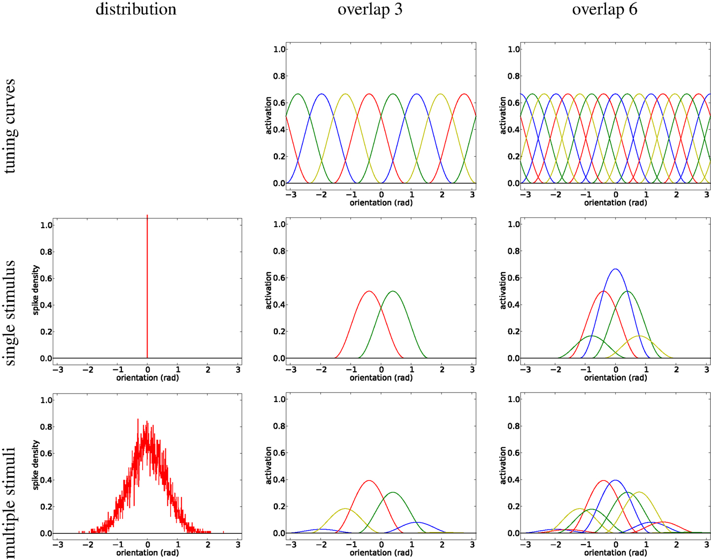
Figure 1. Illustration of population codes/channel representations with minimum overlap (3/middle column) and with overlap 6 (right column). The first row shows the basis functions, the second row shows the encoding (by means of weighted basis functions) of a single stimulus (impulse, cf. left column), and the third row shows the encoding of multiple stimuli (Gaussian distribution, cf. left column).

Population codes have earlier also been referred to as channel codes (Snippe and Koenderink, 1992; Howard and Rogers, 1995) and therefore (and in parallel to recent developments in computational neuroscience), the image processing community has developed the concept of channel representations (Granlund, 2000). Both coding schemes share many similarities, most importantly approximating kernel density estimators in expectation sense (Scott, 1985; Zemel et al., 1998; Felsberg et al., 2006). The tuning curves are referred to as channel basis functions or kernels and the coefficient vectors as channel vectors. Several analytic models, such as Gaussian kernels, cos² kernels, or quadratic B-splines, have been investigated (Forssén, 2004). An overview of channel-based image processing is given in a recent survey (Felsberg, 2012). Other names for population/channel codes are averaged-shifted histograms (Scott, 1985) and distribution fields (Sevilla-Lara and Learned-Miller, 2012; Felsberg, 2013).

The focus in this paper is on decoding channel representations of image information. The purpose of image representations is to turn implicitly existing properties of the underlying image signal into a data structure, a feature descriptor, which makes the properties explicit. For instance, local orientation information is computed from the image signal and combined with color information in a joint feature descriptor used for classification and regression (Felsberg and Hedborg, 2007).

From a statistical point of view, an image representation consists of estimates of the feature components from a set of measurements in the image. These measurements can differ in number, i.e., in the total evidence. The feature component is in most cases assigned the value of the maximum likelihood estimate. In many cases, also the variance of the estimate is considered in terms of coherence (Jähne, 2005).

A good example for the three-folded representation by value/coherence/evidence is the structure tensor (Bigün and Granlund, 1987; Förstner and Gülch, 1987), where the sum of eigenvalues is a measure for the evidence, the difference of eigenvalues (divided by their sum) represents the coherence, and the orientation of the eigenvectors determines the value. It has been pointed out in that the structure tensor results in a 3D cone (Felsberg et al., 2009).¹

One of the major differences between channel representations and population codings is the decoding: the reconstruction from channel codes or the readout from population codes. Channel representations make use of signal processing techniques for local reconstruction (Forssén, 2004), the maximum entropy principle to reconstruct a smoothed density function (Jonsson, 2008), or spline-based mode extraction to find the location with maximum likelihood with a minimum of bias (Felsberg et al., 2006). In contrast, population vector readout uses a recurrent procedure to approximate a maximum-likelihood estimation.

Despite the fact that the readout by means of the population vector estimator is unbiased (Denève et al., 1999), the combination of the recurrent procedure and the estimator becomes biased if the recurrent equation is iterated until convergence. This effect is reduced if the tuning functions overlap extensively and if the recurrent equation is only iterated a few (2–3) times. Both approaches are used in previous work (Denève et al., 1999). However, as pointed out recently (Pellionisz et al., 2013), the recursion of covariant (“proprioception”) vectors always leads to the eigenvectors of the underlying coefficient matrix and is thus a fundamental obstacle for unbiased estimators if iterated to convergence.

In contrast to mentioned previous works, a truly unbiased recurrent network model is derived in the present paper. This is achieved by a theoretical approach and from biologically motivated first principles. The contributions are as follows.

• The analytic form of tuning curves is derived from constancy constraints (Section 2.1).

• The algebraic structure of the resulting minimum-overlap sets is identified. Within this structure, the requirements for unbiased estimates imply Lorentz group constraints on the coefficients (Section 2.2).

• For the decoding of channel vectors with more than three channels, a novel window selection has been derived, establishing a maximum-likelihood estimate (Section 2.3).

• Existing schemes are analyzed with respect to these constraints and a new, unbiased scheme is derived. This scheme is implemented for simulation experiments, where stationary points and bias from noisy image data are compared to existing schemes (Section 2.5).

The presented approaches are based on results from earlier work on channel representations (Sections 2.1 and 2.2) and make use of group theoretic results. The technical details of the work are summarized in the Supplementary Material.

2. Materials and Methods

The current approach to recurrent population codes shows a systematic bias, as we will show further below in this section. This bias can be avoided if the recurrent relations are modified according to certain constraints that we will derive from first principles. These first principles are common practice in many successful image representation techniques.

2.1. Encoding of Population Codes and Minimal Channel Representations

Population codes and channel representations are largely equivalent approaches concerning their encoding properties. In both cases measurements x from a measurements space $\mathcal{M}$ are encoded using channel basis functions b(x) (the tuning curves). These functions are defined on a compact interval, in the case of orientation data, a periodic domain. They are continuous, non-negative, and decay with increasing |x|. The channel support of b is given by the domain where b is non-zero.

The basis function used here is the cos² function, defined as (where h denotes the bandwidth parameter)

$b\left(x\right)=\frac{2}{h}{\cos }^2\left(\mathrm{\pi }x∕h\right)\text{for}\left|x\right|<h∕2\text{and}0\text{otherwise.}$ (1)

Note that we have introduced an additional scaling compared to previous work (Forssén, 2004) to make the basis function mass preserving, see below. The channel basis function is shifted n times (w.l.o.g. by integer displacements) to form the channel basis b(x) with components b_j(x) = b(x – j). The number of non-zero components for any x determines the channel overlap. Computing the components for K measurements x_(k) with weights a_k results in the channel vector c with channel coefficients

$c_j={\displaystyle \sum _{k=0}^{K-1}{a}_{k}b(x_{(k)}-j)}={\displaystyle \sum _{k=0}^{K-1}{a}_k{b}_j(x_{(k)})}j=0\dots n-1.$ (2)

Representing elements of $\mathcal{M}$ using channel vectors is called the channel representation. If the sum of channel coefficients (l₁-norm) is constant 1 for any x, i.e., the channel vector lies in the (n – 1)-simplex, the channel representation is mass preserving. We will only consider such channel representations in the sequel and therefore omit “mass-preserving”. The simplexes for n = 3 and n = 4 are illustrated in Figure 2.

FIGURE 2

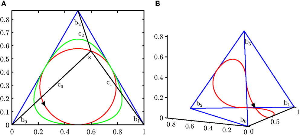
Figure 2. (A) 2-simplex. Blue: edges of a simplex. Red curve: trajectory from cos²-encoded single measurements. Green: B-spline-encoded single measurements. (B) 3-simplex. Blue: edges of simplex. Red: cos²-encoded single measurements.

The channel basis b(x) determines a 1D curve in nD space, parametrized by x. As illustrated in Figure 2, cos² functions result in a circle whereas other basis functions produce less regular shapes (A). Also for n > 3, the cos²-generated curve has constant curvature, but is no longer a circle (B). The circle (n = 3) respectively constant curvatures are direct consequences from the constant l₁- and l₂-norms of b for cos² functions, restricting the curve to be part of the intersection of a plane and a sphere. Averaging channel representations over a set of measurements x_(k) results in a convex combination of points on the curve.

Thus, the cos² channel basis b induces two constancy properties onto the resulting channel vector c: The l₁-norm of c and the l₂-norm of c are independent of displacements of x, as long as x is within the range of the tuning functions. The first property corresponds to the idea of constant probability mass, i.e., each observation provides the same amount of evidence, independently of the specific value. The second property corresponds to the idea of isometry, i.e., scalar products depend only on the relative angle, not on the absolute angle within the reference coordinate system. This property is essential for learning-based approaches that should not be biased toward centers or edges of tuning functions. Thus, both constancy properties are essential for unbiased representations.

A further property of cos² kernels as defined above, with the choice h = 3, is that they have an overlap of three, i.e., for a single observation x, b has three non-zero coefficients:

$\mathbf{\text{b}}(x)={(\dots ,0,\underset{\text{coefficient}[x]-1}{\underbrace{b(x-[x]+1)}},\underset{\text{coefficient}[x]}{\underbrace{b(x-[x])}},\underset{\text{coefficient}[x]+1}{\underbrace{b(x-[x]-1)}},0,\dots )}^{\text{t}},$ (3)

where [x] is the closest integer to x. Together with other standard requirements of kernel functions, we obtain that no kernels exist with overlap smaller than three:

Theorem 2.1. (Minimum-overlap channel basis) The minimum overlap of a channel basis with constant l₂-norm ||b(x)||₂ = μ for all x is 3. $\mathrm{\mu }=\frac{1}{2}$.

Finally, from the two norm constraints, it follows that the cos² kernel, which is the simplest non-constant even function, is the only solution (see Supplementary Material for both proofs):

Theorem 2.2. (Uniqueness of cos²kernel) The unique channel basis function with minimal overlap and integer spacing is given by with equation (1) h = 3.

2.2. Decoding Channel Representations

Three-channel systems have some structural similarities with certain computational color models. Due to the existence of three color receptors on the human retina or color sensors in most cameras, one can describe the raw output of a color imaging system by a three-dimensional vector (usually in some form of RGB space), which is structurally similar to the channel vectors introduced above. In this spirit, the color opponent transform (Lenz and Carmona, 2010; van de Sande et al., 2010) and its variant in cylindrical coordinates, i.e., hue–saturation–intensity (van de Weijer et al., 2005), are three-folded representations, see Section 1. In Figure 3, the color opponent transform, an orthogonal transformation of RGB, is illustrated.

FIGURE 3

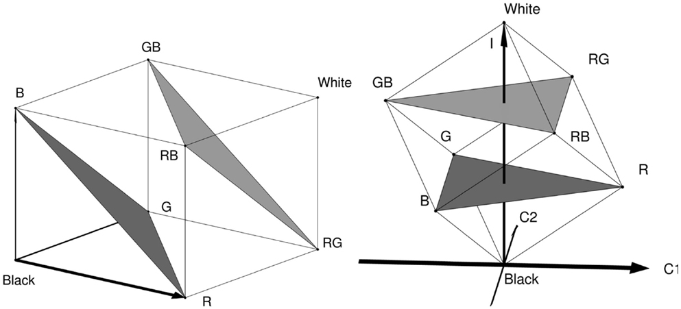
Figure 3. Illustration of the color opponent transform (Åström, 2015). Figure courtesy Freddie Åström.

The concept of three-folded representations by value/coherence/evidence has been related to channel representations, and thus population codes, in context of decoding cos² channels (Forssén, 2004), from which we have adopted the notation in Figure 4: value $\widehat{x}$, coherence ${\widehat{r}}_1∕{\widehat{r}}_2$, and evidence ${\widehat{r}}_2$. Previous work refers to ${\widehat{r}}_1$ and ${\widehat{r}}_2$ as confidence measures and suggests to form the 3-vector $\mathbf{\text{p}}={\left(p_0,p_1,p_2\right)}^{\text{t}}:={\left({\widehat{r}}_1\cos 2\pi \widehat{x}∕3,{\widehat{r}}_1\sin 2\pi \widehat{x}∕3,{\widehat{r}}_2\right)}^{\text{t}}$ using a matrix of orthogonal column vectors W^t = (w₀, w₁, w₂). After normalization², we obtain:

$\mathbf{\text{c}}={\mathbf{\text{W}}}^{\text{t}}\mathbf{\text{p}}:=\frac{1}{\sqrt{3}}\left(\begin{array}{ccc}\hfill \sqrt{2}\hfill & \hfill 0\hfill & \hfill 1\hfill \\ \hfill \sqrt{2}\cos \left(2\pi ∕3\right)\hfill & \hfill \sqrt{2}\sin \left(2\pi ∕3\right)\hfill & \hfill 1\hfill \\ \hfill \sqrt{2}\cos \left(4\pi ∕3\right)\hfill & \hfill \sqrt{2}\sin \left(4\pi ∕3\right)\hfill & \hfill 1\hfill \end{array}\right)\left(\begin{array}{c}\hfill r_1\cos \left(2\pi x∕3\right)\hfill \\ \hfill r_1\sin \left(2\pi x∕3\right)\hfill \\ \hfill r_2\hfill \end{array}\right)$ (4)

FIGURE 4

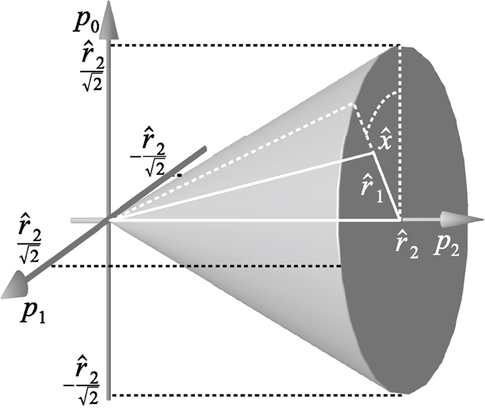
Figure 4. The 3D cone formed by evidence ${\widehat{\mathit{\text{r}}}}_2$, coherence ${\widehat{\mathit{\text{r}}}}_1∕{\widehat{\mathit{\text{r}}}}_2$, and value $\widehat{\mathit{\text{x}}}$.

Inverting this expression gives p = Wc, and the estimate for x is obtained by extracting the phase-angle

$\widehat{x}=\frac{3}{2\pi }\arg \left(p_0+i{p}_1\right)=\frac{3}{2\pi }\arg \left({\mathbf{\text{c}}}^{\text{t}}\left({\mathbf{\text{w}}}_0+i{\mathbf{\text{w}}}_1\right)\right).$ (5)

Thus, all involved operations (matrix-vector products and extraction of phase) are the same as for the readout of population codes (Denève et al., 1999) and are biologically plausible (Mechler et al., 2002).

Note that the normalization of the matrix columns implies that $r_2=\sqrt{2}{r}_1$ in the case of a single encoded value. Thus, the cone becomes acute (70.5° instead of 90°). If a set of measurements is represented using channels, the resulting channel vector c is a convex combination of points on the surface of this cone, i.e., a point in the interior of the cone, and $r_2>\sqrt{2}{r}_1$ in general. Decoding this channel vector is then related to finding the closest point on the cone surface. The exact definition of closest in this context is dependent on the transformation group considered. Using just p₀ and p₁ as suggested previously (Forssén, 2004) means to neglect distances along p₂.

The three-fold representations above live in a cone, i.e., if representations are modified or compared, the transformations that leave the cone invariant need to be analyzed and represented. Obviously, we may not use Euclidean transformations for this purpose, because they would produce results outside the cone. Instead, we consider Lorentz transformations similar to those we know from relativity theory.³

In our case, the Lorentz transformations consist of rotations about the cone axis and Lorentz boosts (contractions). The rotation about the cone axis corresponds to changes of our measurements x (see also Figure 4), thus an unbiased scheme must be rotation invariant. Using the change of coordinates from the previous section, we derive a constraint on the update of c that must be fulfilled in each step of a recurrent scheme (the proof is given in Supplementary Material):

Theorem 2.3. (Constraint on channel coefficients) The decoding of a 3-channel vector c is invariant under a change of channel coefficients ${\nabla }_{\mathbf{\text{c}}}={\left({\partial }_{c_0},{\partial }_{c_1},{\partial }_{c_2}\right)}^{\text{t}}$ iff

$\left(c_0-c_1\right){\partial }_{c_2}+\left(c_2-c_0\right){\partial }_{c_1}+\left(c_1-c_2\right){\partial }_{c_0}=0.$ (6)

2.3. Windowed Decoding by Maximum-Likelihood Estimation

The decoding based on equation (5) is defined for channel representations with three channels. For the general case of more than three channels, recurrent schemes will be discussed below. However, non-iterative methods for more than three channels have been suggested (Forssén, 2004), based on first selecting a window of three channels and then applying equation (4).

The 3-window is selected by various criteria, e.g., maximizing r₂ or having a local maximum at the center channel c_j−1 ≤ c_j ≥ c_j+1. From a statistical point of view, however, a maximum-likelihood selection would be preferable and under the assumption of independent Gaussian noise, we arrive at a least squares problem and the corresponding theorem (the proof is given in Supplementary Material):

Theorem 2.4. (Maximum-likelihood decoding) Assuming independent Gaussian noise on the channel coefficients, the decoding 3-window with maximum likelihood is given at the index j

$\widehat{j}=\arg \underset{j}{\max }{\tilde{r}}_1\left(j\right)+\sqrt{2}{r}_2\left(j\right),$ (7)

where r_i(j) is computed as r_i of the vector c_j : = (c_j−1, c_j, c_j+1)^t,

${\tilde{r}}_1\left(j\right)=\left\{\begin{array}{cc}{r}_1\left(j\right)\hfill & \text{if}\left|\mathrm{\alpha }\left({\mathbf{\text{c}}}_j\right)\right|\le \mathrm{\pi }∕3\hfill \\ r_1\left(j\right)\cos \left(\left|\mathrm{\alpha }\left({\mathbf{\text{c}}}_j\right)\right|-\mathrm{\pi }∕3\right)\hfill & \text{else},\hfill \end{array}\right.$ (8)

and $\mathrm{\alpha }\left({\mathbf{\text{c}}}_j\right)=\arg \left({\mathbf{\text{c}}}_j^{\text{t}}\left({\mathbf{\text{w}}}_0+i{\mathbf{\text{w}}}_1\right)\right)-\frac{2\pi }{3}$. The MLE is given as $\widehat{x}=\max \left(\min \left(\frac{3}{2\pi }\mathrm{\alpha }\left({\mathbf{\text{c}}}_{\widehat{j}}\right),\frac{1}{2}\right),-\frac{1}{2}\right)+\widehat{j}$.

2.4. Analysis of the Existing Recurrent Scheme for Population Codes

The recurrent procedure suggested for the readout of population codes (Denève et al., 1999) contains the same building blocks as channel decoding and is biologically equally plausible, because such procedures coincide with cortical circuitry. It is suggested to establish two coupled, non-linear equations, the first one being a linear mapping of the population vector o to a slack vector u = Ao, and the second one writing back the squared and normalized u into o:

$o_j=u_j^2∕\left(S+\mathrm{\mu }|\mathbf{\text{u}}{|}^2\right).$ (9)

The computational flow of this method is illustrated in Figure 5.

FIGURE 5

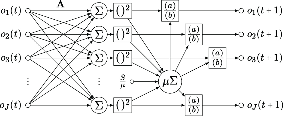
Figure 5. Diagram of the recurrent network for the readout of population codes (Denève et al., 1999).

The problem is, however, that the scheme given in equation (9) only fulfills the invariance requirement (6) in one trivial case for A. In all other cases, iterating through the scheme leads to successively larger bias toward specific values, e.g., at the channel centers (the proof is given in Supplementary Material):

Theorem 2.5. (Bias of Denève’s scheme) The scheme (9) is biased unless we choose

$\mathbf{\text{A}}=\sqrt{\frac{S}{3\left(1-\mathrm{\mu }\right)}}\left(\begin{array}{ccc}\hfill 1\hfill & \hfill 1\hfill & \hfill 1\hfill \\ \hfill 1\hfill & \hfill 1\hfill & \hfill 1\hfill \\ \hfill 1\hfill & \hfill 1\hfill & \hfill 1\hfill \end{array}\right),\mathit{where}\mathrm{\mu }<1.$ (10)

2.5. The New Recurrent Scheme

In this section, we will derive a recurrent scheme that, in contrast to equation (9), fulfills the invariance constraint for the value (6). Moreover, a recurrent scheme should not modify the evidence either, i.e., we require

${\partial }_{r_2}={\mathbf{\text{w}}}_2^{\text{t}}{\nabla }_{\mathbf{\text{c}}}=0.$ (11)

The two constraints (6) and (11) imply the existence of a solution in terms of their common null-space. In the case of three channels, this space is spanned by permutations of the vector (−1, 2, −1)^t, the (negative) discrete Laplacian kernel. Since the update of c in the corresponding scheme has to be in a (3-2)-D subspace, only one degree of freedom exists and is uniquely determined by the requirement $\sqrt{2}{r}_1=r_2$.

Thus, the fixpoint solution can be achieved by a single computation and suitable δ as

${\mathbf{\text{c}}}_0=\mathbf{\text{c}}+\mathrm{\delta }\left(\begin{array}{ccc}\hfill 2\hfill & \hfill -1\hfill & \hfill -1\hfill \\ \hfill -1\hfill & \hfill 2\hfill & \hfill -1\hfill \\ \hfill -1\hfill & \hfill -1\hfill & \hfill 2\hfill \end{array}\right)\mathbf{\text{c}}.$ (12)

In the case of more than three channels, the algebraic structure becomes more complicated, because points are no longer projected onto a circle in the plane, but onto a 1-D curve in high-dimensional space. This can no longer be achieved by a linear equation as in equation (12). The proper generalization is obtained by splitting the Laplacian operator according to $\mathrm{\Delta }={\partial }_j^2$ (j being the index of c, thus ∂_j being the finite difference operator) and defining d = ∂_jc as the flow between the channels in each incremental step c_t

${\mathbf{\text{c}}}_t\propto {\partial }_j\mathbf{\text{d}},$ (13)

establishing the continuity equation of channel coefficients. The flow coefficient d_j determines how much of the coefficient c_j is moved to c_j+1.

In contrast to equation (12), where the flow is computed by the difference c_j+1−c_j, the case of more than three channels requires a non-linear mapping f: $\mathbb{R}$² →$\mathbb{R}$; $\left(c_j,c_{j+1}\right)\mapsto d_j$ to compute the flow. The complete computational scheme is illustrated in Figure 6.

FIGURE 6

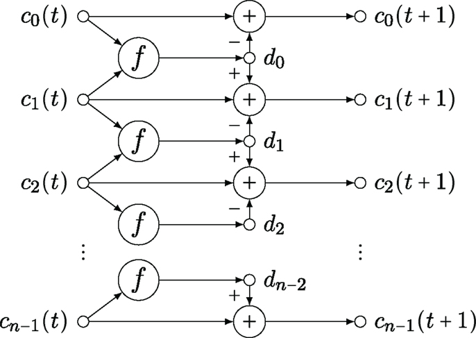
Figure 6. Diagram of the proposed recurrent network. f is the function to compute the flow.

Assuming that the function f is known and δ being the update step length, we obtain the following iterative algorithm:

 while $\sqrt{2}{r}_1<r_2$ do
  for all j do
   dj ← f (cj, cj+1)
  end for
  for all j do
   cj ← cj + δ(dj–1 – dj)
  end for
 end while

The implementation of such a scheme and the comparison to the state-of-the-art scheme (Denève et al., 1999) with respect to stationary points using simulation data and with respect to bias using noisy image data is shown in the subsequent section.

3. Results

In this section, we analyze stationary points of the discussed recurrent schemes and we perform experiments on orientation analysis from noisy images. Before looking into the iterative schemes, we first compare the non-iterative decoding according to maximum r₂ (Forssén, 2004) and Theorem 2.4, see Figure 7. In the experiment, we compare the respective decoding result for 1000 random measurements encoded into 7 channels and combined with random weights. Obviously, the modification of the window selection leads to exact reproduction of MLE results.

FIGURE 7

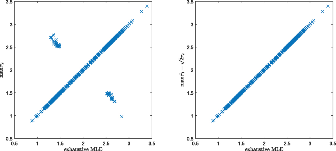
Figure 7. Comparison between decoding maximizing r₂ (Forssén, 2004), left, and the proposed MLE according to Theorem 2.4, right. 1000 random measurements have been generated with random weights and encoded with 7 channels.

3.1. Stationary Points Analysis

A fully unbiased recurrent scheme must keep the entire measurement domain invariant, i.e., each point in the measurement space is a stationary point under the recurrent scheme. For this subsection, we restrict the discussion to the case of three orientation channels.

In the case of Denève’s scheme, we already know from Theorem 2.5 that only one trivial solution exists. However, we can calculate which discrete points are stationary points by requiring

$\mathbf{\text{o}}\left(t+1\right)=\mathbf{\text{o}}\left(t\right).$ (14)

If o is a stationary point, u = Ao is constant, and thus, also the normalization factor Q : = S + μ|u|² is constant. As in the proof of Theorem 2.5, we exploit that A is circulant, but it is also symmetric (we may reflect all vectors) and thus

$\mathbf{\text{A}}=\left(\begin{array}{ccc}\hfill \mathrm{\alpha }\hfill & \hfill \mathrm{\beta }\hfill & \hfill \mathrm{\beta }\hfill \\ \hfill \mathrm{\beta }\hfill & \hfill \mathrm{\alpha }\hfill & \hfill \mathrm{\beta }\hfill \\ \hfill \mathrm{\beta }\hfill & \hfill \mathrm{\beta }\hfill & \hfill \mathrm{\alpha }\hfill \end{array}\right)$ (15)

for suitable α and β. For a stationary solution, we obtain $o_j=\frac{1}{Q}{\left(\mathbf{\text{Ao}}\right)}_j^2$ and therefore

$\begin{array}{c}\hfill o_0=\frac{1}{Q}{\left(\mathrm{\alpha }{o}_0+\mathrm{\beta }{o}_1+\mathrm{\beta }{o}_2\right)}^2\hfill \\ \hfill o_1=\frac{1}{Q}{\left(\mathrm{\beta }{o}_0+\mathrm{\alpha }{o}_1+\mathrm{\beta }{o}_2\right)}^2\hfill \\ \hfill o_2=\frac{1}{Q}{\left(\mathrm{\beta }{o}_0+\mathrm{\beta }{o}_1+\mathrm{\alpha }{o}_2\right)}^2\hfill \end{array}.$ (16)

Q only affects absolute scale of stationary points, as does simultaneously scaling of α and β. Thus, only one degree of freedom remains for changing the stationary points: the quotient of β/α.

Without loss of generality, we now set S = 0.1, μ = 0.9, and α = 1. For different choices of β, we can now plot the trajectories under iterations of equation (9), see Figure 8. For comparison, we also include the result from our proposed method (12).

FIGURE 8

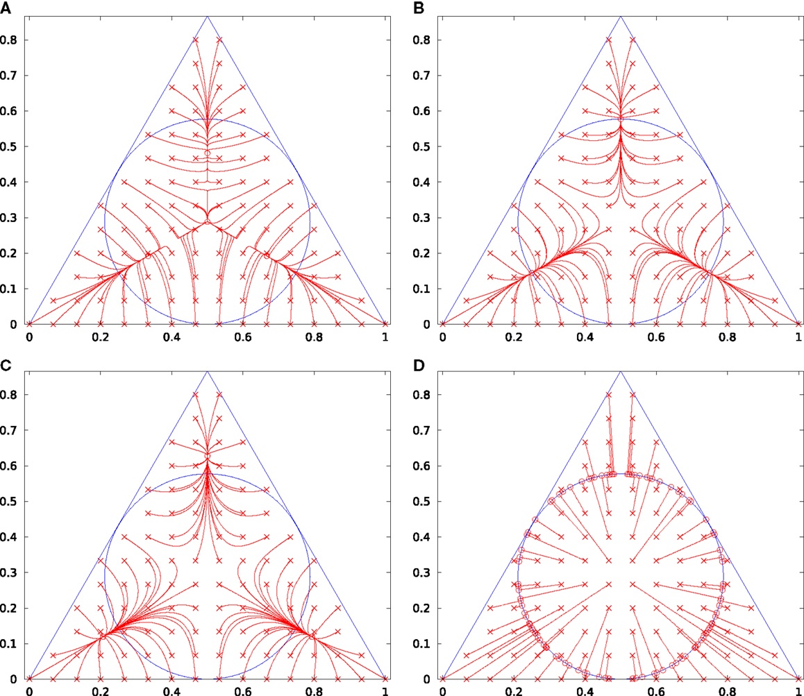
Figure 8. Three-channel iterative processing. The original samples are indicated by crosses, the convergence points by circles. The results of Denève’s iterative method are shown in (A) (β = 0.26α), (B) (β = 0.25α), and (C) (β = 0.24α). The result of our method (12) is shown in (D).

Obviously, Denève’s method has a discrete set of stationary points, which means that iterating until convergence will lead to one out of a set of discrete solutions and thus, the result is strongly biased. Our solution for three channels, however, maps to all points on the unit circle and is thus unbiased.

3.2. Orientation Estimation from Image Data

In this section, we perform a number of experiments using two sets of visual stimuli with different complexity: one contains a single orientation without texture (Hubel and Wiesel, 1959), see Figure 9A, and the other one multiple orientations with varying textures (Felsberg et al., 2006), see Figure 10A. From rotated and noisy instances of these images, local orientation information is extracted with a regularized gradient filter (Scharr et al., 1997). The color coded orientation data is illustrated in Figures 9 and 10B.

FIGURE 9

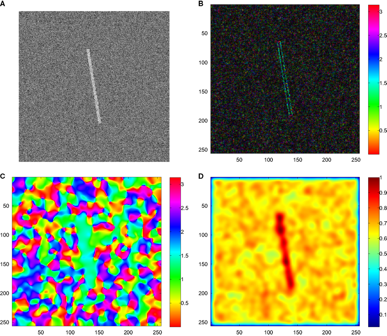
Figure 9. Orientation experiment with a simple stimulus (Hubel and Wiesel, 1959). (A) Example pattern with noise. (B) Raw orientation estimates computed with the Scharr filter (Scharr et al., 1997). (C) Channel smoothed orientation estimates (Felsberg et al., 2006). (D) Weighted coherence $\left({\widehat{r}}_1\right)$ of the estimate. The subsequent evaluation is made in the center point (128,128).

FIGURE 10

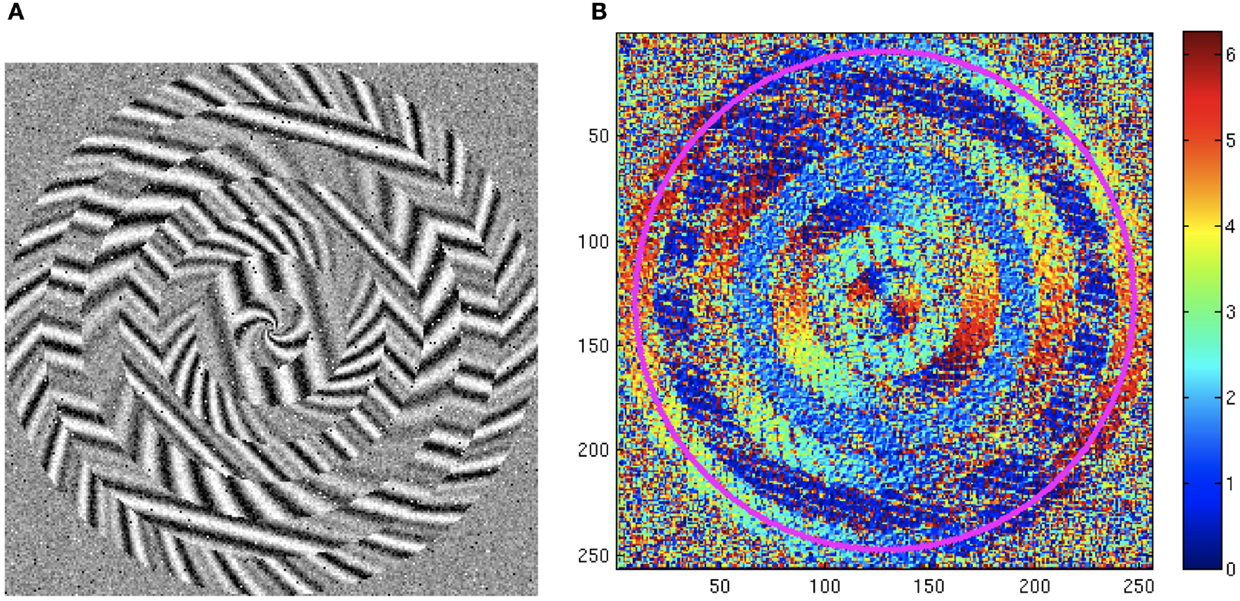
Figure 10. Orientation experiment with a complex pattern (Felsberg et al., 2006). (A) Example pattern with noise. (B) Raw orientation estimates computed with the Scharr filter (Scharr et al., 1997). The subsequent evaluation is made along the magenta circle.

The extracted orientation estimates are pixel-wise channel coded and the resulting channel images are spatially averaged (Felsberg et al., 2006). The resulting channel representations are then decoded; the result is shown in Figures 11 and 12A. If we apply 5, 10, and 100 iterations according to equation (9) before decoding, the results as shown in Figures 11 and 12B–D, respectively, are obtained. It is obvious for all cases that the iterative scheme (9) leads to an increasing bias. For three channels, the case of decoding without iterating (9) corresponds to our solution (12) and shows no significant bias.

FIGURE 11

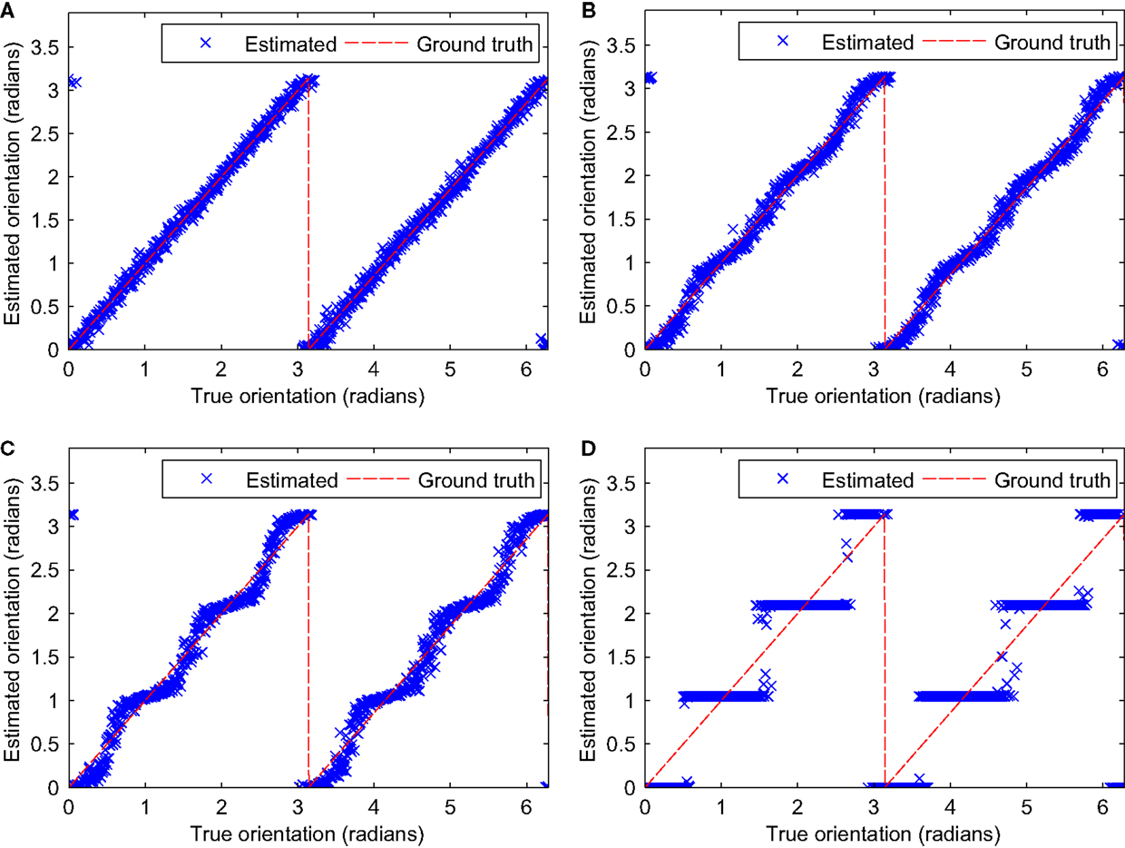
Figure 11. Evaluation results using stimuli from Figure 9 for three channels. (A–D) decoding with respectively 0, 5, 10, and 100 iterations according to (9).

FIGURE 12

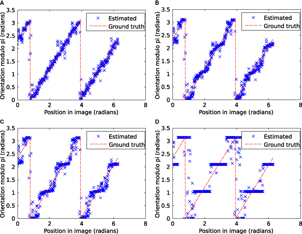
Figure 12. Evaluation results using stimuli from Figure 10 for three channels. (A–D) decoding with respectively 0, 5, 10, and 100 iterations according to (9).

In Figure 13, the corresponding results are shown for 7 channels. The used basis functions are displayed in Figure 13A. The look-up table for the flow function f (c_j, c_j+1) between the channels is displayed in Figure 13B. The look-up table is generated by successively low-pass filtering random samples from a Gaussian distribution, computing the flow, and inverting the sign. The result from the proposed iterative scheme shows no bias effect if iterated to convergence (see Figures 13D,F) whereas Denève’s method shows clearly visible bias effects (cf. Figures 13C,E).

FIGURE 13

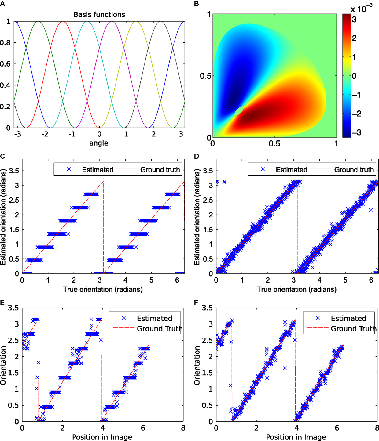
Figure 13. Evaluation results: Stimuli from Figures 9 and 10, seven channels, repeated until convergence. (A) Basis functions used in all experiments with seven channels. (B) Plot of look-up table for the function f (c_j, c_j+1) to compute the flow according to Figure 6. (C,E) Iterations using (9). (D,F) Iterations using (13) and look-up table. (C,D) Input pattern from Figure 9. (E,F) Input pattern from Figure 10.

So far, the advantage of applying the proposed scheme compared to direct decoding has not been very explicit. This changes if the noise distribution becomes broader. In Figure 14, we show results for simulations with orientation samples (200, respectively, 1800) drawn from a distribution with standard deviation of 0.5 respectively 1.5 times the decoding window width. 10 iterations of Denève’s method result already in a clearly visible bias (Figures 14C,D), whereas the proposed scheme shows no bias in either case (Figures 14E,F). The direct decoding shows no visible bias for the narrower distribution (a) and a clearly visible bias for the wider distribution (b). Note that the bias may not be evaluated if the mean of the distribution is placed at a channel center or at a boundary. For such setups, all methods show an unbiased behavior.

FIGURE 14

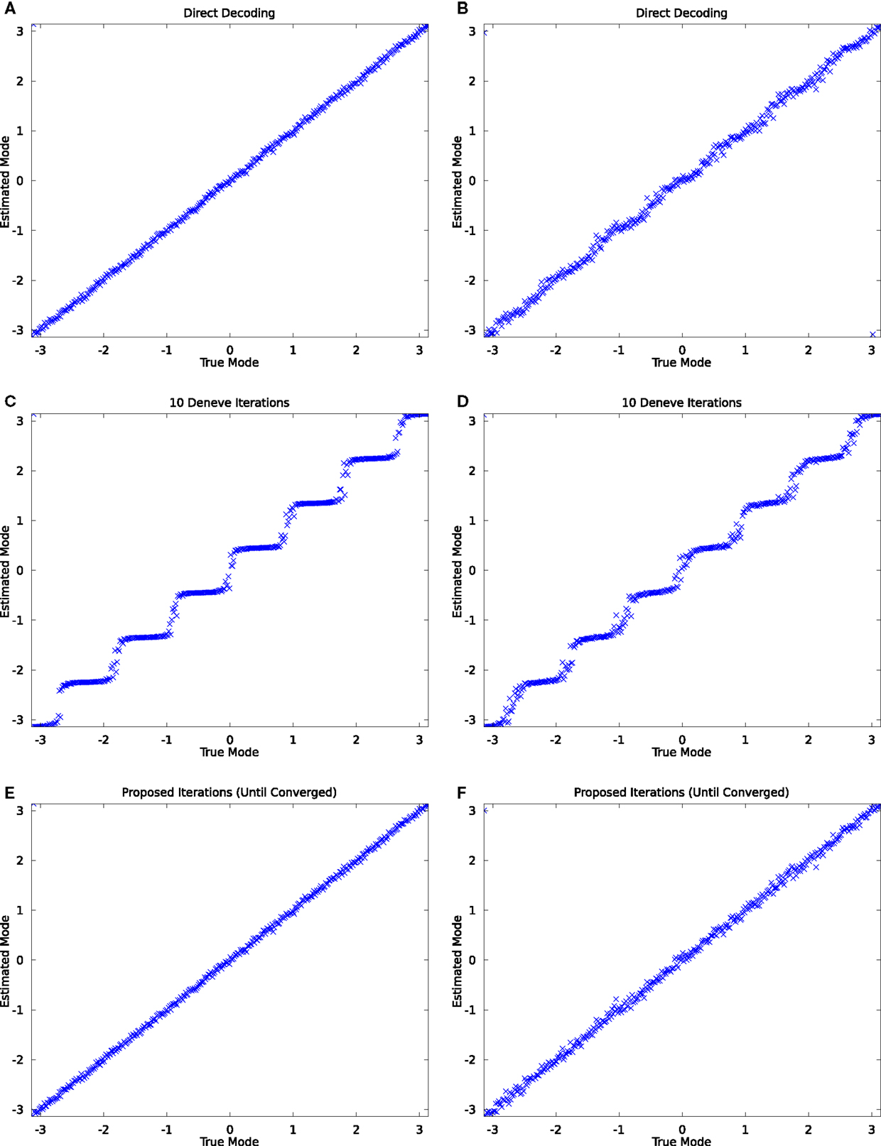
Figure 14. Simulation of orientation information with varying standard deviations. (A,C,E): results for σ = half the decoding window, 200 samples; (B,D,F) for σ = 1.5 times the decoding window, 1800 samples. (A,B): decoding without iterations; (C,D) results using 10 iterations of (9); (E,F) results using the proposed scheme.

4. Discussion

We have shown that the recurrent scheme by Denève produces biased output if the mean of the stimuli is not located on a channel center or a channel boundary and if the recurrent scheme is iterated until convergence. The bias of Denève’s method has not been visible in the original paper (Denève et al., 1999), because all evaluations have been done either on data centered at a stationary point or as averaged error over all distribution centers.

The suggested extensive overlap of tuning functions and fixed number of iterations (Denève et al., 1999) lead only to a gradual reduction of the bias and have three major practical drawbacks for the design of computational systems:

1. The extensive overlap of tuning functions (oversampling in signal processing terms) increases the redundancy, and thus the computational effort.

2. The number of iterations depends on the noise level of the input: noisier data requires longer processing time as observed in biological systems. Reducing the number of iterations to a fixed number (in order to limit the bias) will result in useless output if the noise level is above a certain threshold.

3. Dynamic processes with continuous input, i.e., using population codes as an implementation of a Kalman filter (Denève et al., 2007), will make use of the iterative procedure in each time step, and thus the recurrent equation is potentially applied an arbitrary number of times, eventually leading to biased estimates.

All three drawbacks are avoided by using the proposed channel-based approach, established by means of theorems 2.1–2.4 and a simple look-up table. Besides the fact of establishing a new theoretical and computational model for recurrent networks, this possibly leads to two new applications:

• Application 1: denoising for learning – many channel-based learning algorithms (Felsberg et al., 2013) require clean inputs in order to avoid responses to insignificant inputs. If the recurrent scheme is applied before the training, cleaner responses might be the consequence.

• Application 2: adaptive channel resolutions – in certain cases, it would be useful to increase resolution of the channel representation during processing (Felsberg, 2010). This requires a sharpening of the underlying measured distribution, which can be achieved by the proposed scheme.

In conclusion, we believe that recurrent networks are very useful tools, but have to be applied in the appropriate way in order to avoid introducing unwanted bias effects.

Author Contributions

MF has been the lead-researcher in this work, developing most of the conceptual ideas, proving most of the theorems, and writing most of the text. KÖ has been contributing with ideas concerning decoding-invariant processing, deriving computational schemes, running simulations, and contributing to the text. RL has been contributing with derivations and explanations on Lorentz groups and group theory, in general, including the respective sections of the text.

Funding

This work has been supported by the VR projects EMC² and VIDI, by the SSF projects CUAS and VPS, and by the excellence centers ELLIIT and CADICS.

Conflict of Interest Statement

The authors declare that the research was conducted in the absence of any commercial or financial relationships that could be construed as a potential conflict of interest.

Supplementary Material

The Supplementary Material for this article can be found online at https://www.frontiersin.org/article/10.3389/frobt.2015.00020

Footnotes

1. ^Other examples for the three-folded representation are based on local phase estimates, where the coherence (phase-congruency) may be used for simultaneous detection of lines and edges (Reisfeld, 1996; Kovesi, 1999; Felsberg et al., 2005), and color (Lenz and Carmona, 2010). In the latter case, the evidence determines intensity, the coherence is a saturation measure, and the value represents the hue.
2. ^For the sake of convenience, we use the normalized coefficient matrix as common in literature (Fässler and Stiefel, 1992; Lenz and Carmona, 2010)
3. ^The cone geometry is easiest defined in (2 + 1)D Minkowski space ${\mathbb{R}}^{2,1}$. The associated quadratic form has the signature {+, +, − 1}, i.e., $p_0^2+p_1^2-p_2^2$. The transformation group that we consider is the special orthogonal group, SO(2,1), more accurately the connected component SO⁺(2,1).

References

Azzopardi, G., and Petkov, N. (2013). Trainable COSFIRE filters for keypoint detection and pattern recognition. IEEE Trans. Pattern Anal. Mach. Intell. 35, 490–503. doi: 10.1109/TPAMI.2012.106

PubMed Abstract | CrossRef Full Text | Google Scholar

Azzopardi, G., and Petkov, N. (2014). Ventral-stream-like shape representation: from pixel intensity values to trainable object-selective cosfire models. Front. Comput. Neurosci. 8:80. doi:10.3389/fncom.2014.00080

PubMed Abstract | CrossRef Full Text | Google Scholar

Åström, F. (2015). Variational Tensor-Based Models for Image Diffusion in Non-Linear Domains. Ph.D. thesis, Linköping University, Sweden.

Google Scholar

Bigün, J., and Granlund, G. H. (1987). “Optimal orientation detection of linear symmetry,” in Proceedings of the IEEE First International Conference on Computer Vision (London: IEEE), 433–438.

Google Scholar

Dalal, N., and Triggs, B. (2005). “Histograms of oriented gradients for human detection,” in Computer Vision and Pattern Recognition (CVPR) 2005. IEEE Computer Society Conference on, Vol. 1 (San Diego, CA: IEEE), 886–893. doi:10.1109/CVPR.2005.177

CrossRef Full Text | Google Scholar

d’Angelo, E., Alahi, A., and Vandergheynst, P. (2012). “Beyond bits: reconstructing images from local binary descriptors,” in Pattern Recognition (ICPR), 2012 21st International Conference on (Tsukuba: IEEE), 935–938.

Google Scholar

Denève, S., Duhamel, J.-R., and Pouget, A. (2007). Optimal sensorimotor integration in recurrent cortical networks: a neural implementation of Kalman filters. J. Neurosci. 27, 5744–5756. doi:10.1523/JNEUROSCI.3985-06.2007

PubMed Abstract | CrossRef Full Text | Google Scholar

Denève, S., Latham, P. E., and Pouget, A. (1999). Reading population codes: a neural implementation of ideal observers. Nat. Neurosci. 2, 740–745. doi:10.1038/11205

PubMed Abstract | CrossRef Full Text | Google Scholar

Fässler, A., and Stiefel, E. (1992). “Preliminaries,” in Group Theoretical Methods and Their Applications. Boston, MA: Birkhäuser, 1–31.

Google Scholar

Felsberg, M. (2010). “Incremental computation of feature hierarchies,” in Pattern Recognition 2010, Proceedings of the 32nd DAGM, Darmstadt.

Google Scholar

Felsberg, M. (2012). “Chap. Adaptive filtering using channel representations,” in Mathematical Methods for Signal and Image Analysis and Representation, volume 41 of Computational Imaging and Vision, eds L. Florack, R. Duits, G. Jongbloed, M. C. van Lieshout, and L. Davies (London: Springer), 31–48.

Google Scholar

Felsberg, M. (2013). “Enhanced distribution field tracking using channel representations,” in IEEE ICCV Workshop on Visual Object Tracking Challenge, Sydney.

Google Scholar

Felsberg, M., Duits, R., and Florack, L. (2005). The monogenic scale space on a rectangular domain and its features. Int. J. Comput. Vis. 64, 187–201. doi:10.1007/s11263-005-1843-x

CrossRef Full Text | Google Scholar

Felsberg, M., Forssén, P.-E., and Scharr, H. (2006). Channel smoothing: efficient robust smoothing of low-level signal features. IEEE Trans. Pattern Anal. Mach. Intell. 28, 209–222. doi:10.1109/TPAMI.2006.29

PubMed Abstract | CrossRef Full Text | Google Scholar

Felsberg, M., and Hedborg, J. (2007). Real-time view-based pose recognition and interpolation for tracking initialization. J. R. Time Image Process. 2, 103–116. doi:10.1007/s11554-007-0044-y

CrossRef Full Text | Google Scholar

Felsberg, M., Kalkan, S., and Krüger, N. (2009). Continuous dimensionality characterization of image structures. Image Vis. Comput. 27, 628–636. doi:10.1016/j.imavis.2008.06.018

CrossRef Full Text | Google Scholar

Felsberg, M., Larsson, F., Wiklund, J., Wadstromer, N., and Ahlberg, J. (2013). Online learning of correspondences between images. IEEE Trans. Pattern Anal. Mach. Intell. 35, 118–129. doi:10.1109/TPAMI.2012.65

PubMed Abstract | CrossRef Full Text | Google Scholar

Forssén, P. E. (2004). Low and Medium Level Vision using Channel Representations. PhD thesis, Linköping University, Sweden.

Google Scholar

Förstner, W., and Gülch, E. (1987). “A fast operator for detection and precise location of distinct points, corners and centres of circular features,” in ISPRS Intercommission Workshop (Interlaken: ISPRS), 149–155.

Google Scholar

Granlund, G. H. (2000). “An associative perception-action structure using a localized space variant information representation,” in Proc. Int. Workshop on Algebraic Frames for the Perception-Action Cycle (Heidelberg: Springer).

Google Scholar

Howard, I. P., and Rogers, B. J. (1995). Binocular Vision and Stereopsis. Oxford: Oxford University Press.

Google Scholar

Hubel, D. H., and Wiesel, T. N. (1959). Receptive fields of single neurones in the cat’s striate cortex. J. Physiol. 148, 574–591. doi:10.1113/jphysiol.1959.sp006308

CrossRef Full Text | Google Scholar

Jähne, B. (2005). Digital Image Processing, 6th Edn. Berlin: Springer.

Google Scholar

Jonsson, E. (2008). Channel-Coded Feature Maps for Computer Vision and Machine Learning. Ph.D. thesis, Linköping University, Sweden. Dissertation No. 1160, ISBN 978-91-7393-988-1.

Google Scholar

Kato, H., and Harada, T. (2014). “Image reconstruction from bag-of-visual-words,” in 2014 IEEE Conference on Computer Vision and Pattern Recognition (CVPR) (Columbus: IEEE), 955–962.

Google Scholar

Kovesi, P. (1999). Image features from phase information. Videre J. Comput. Vis. Res. 1, 1–26.

Google Scholar

LeCun, Y., and Bengio, Y. (1995). Convolutional networks for images, speech, and time series. Handb. Brain Theory Neural Netw. 3361, 255–258.

Google Scholar

Lenz, R., and Carmona, P. L. (2010). “Hierarchical s(3)-coding of rgb histograms,” in Computer Vision, Imaging and Computer Graphics. Theory and Applications, Vol. 68 of Communications in Computer and Information Science, eds A. Ranchordas, J. M. Pereira, H. J. Araújo and J. M. R. S. Tavares (Berlin: Springer), 188–200.

Google Scholar

Lowe, D. G. (2004). Distinctive image features from scale-invariant keypoints. Int. J. Comput. Vis. 60, 91–110. doi:10.1023/B:VISI.0000029664.99615.94

PubMed Abstract | CrossRef Full Text | Google Scholar

Mahendran, A., and Vedaldi, A. (2015). Understanding deep image representations by inverting them. The IEEE Conference on Computer Vision and Pattern Recognition (CVPR), Boston, MA.

Google Scholar

Mechler, F., Reich, D. S., and Victor, J. D. (2002). Detection and discrimination of relative spatial phase by V1 neurons. Journal of Neuroscience 22, 6129–6157.

PubMed Abstract | Google Scholar

Pellionisz, A., Graham, R., Pellionisz, P., and Perez, J.-C. (2013). “Recursive genome function of the cerebellum: geometric unification of neuroscience and genomics,” in Handbook of the Cerebellum and Cerebellar Disorders, eds M. Manto, J. Schmahmann, F. Rossi, D. Gruol, and N. Koibuchi (Netherlands: Springer), 1381–1423.

Google Scholar

Pouget, A., Dayan, P., and Zemel, R. (2000). Information processing with population codes. Nat. Rev. Neurosci. 1, 125–132. doi:10.1038/35039062

PubMed Abstract | CrossRef Full Text | Google Scholar

Reisfeld, D. (1996). The constrained phase congruency feature detector: simultaneous localization, classification and scale determination. Pattern Recognit. Lett. 17, 1161–1169. doi:10.1016/0167-8655(96)00081-5

CrossRef Full Text | Google Scholar

Scharr, H., Körkel, S., and Jähne, B. (1997). “Numerische isotropieoptimierung von FIR-Filtern mittels Querglättung,” in DAGM Symposium Mustererkennung, eds E. Paulus and F. M. Wahl (Braunschweig: Springer), 367–374.

Google Scholar

Scott, D. W. (1985). Averaged shifted histograms: effective nonparametric density estimators in several dimensions. Ann. Stat. 13, 1024–1040. doi:10.1214/aos/1176349654

CrossRef Full Text | Google Scholar

Sevilla-Lara, L., and Learned-Miller, E. (2012). “Distribution fields for tracking,” in Computer Vision and Pattern Recognition (CVPR), 2012 IEEE Conference on (Providence, RI: IEEE), 1910–1917. doi:10.1109/CVPR.2012.6247891

CrossRef Full Text | Google Scholar

Snippe, H. P., and Koenderink, J. J. (1992). Discrimination thresholds for channel-coded systems. Biol. Cybern. 66, 543–551. doi:10.1007/BF00204120

PubMed Abstract | CrossRef Full Text | Google Scholar

van de Sande, K., Gevers, T., and Snoek, C. (2010). Evaluating color descriptors for object and scene recognition. IEEE Trans. Pattern Anal. Mach. Intell. 32, 1582–1596. doi:10.1109/TPAMI.2009.154

PubMed Abstract | CrossRef Full Text | Google Scholar

van de Weijer, J., Gevers, T., and Geusebroek, J.-M. (2005). Edge and corner detection by photometric quasi-invariants. IEEE Trans. Pattern Anal. Mach. Intell. 27, 625–630. doi:10.1109/TPAMI.2005.75

PubMed Abstract | CrossRef Full Text | Google Scholar

Vondrick, C., Khosla, A., Malisiewicz, T., and Torralba, A. (2013). “HOGgles: visualizing object detection features,” in ICCV, Sydney.

Google Scholar

Weinzaepfel, P., Jegou, H., and Perez, P. (2011). “Reconstructing an image from its local descriptors,” in Computer Vision and Pattern Recognition (CVPR), 2011 IEEE Conference on (IEEE: Colorado Springs), 337–344.

Google Scholar

Zeiler, M., and Fergus, R. (2014). “Visualizing and understanding convolutional networks,” in Computer Vision – ECCV 2014, volume 8689 of Lecture Notes in Computer Science, eds D. Fleet, T. Pajdla, B. Schiele, and T. Tuytelaars (Zürich: Springer International Publishing), 818–833.

Google Scholar

Zemel, R. S., Dayan, P., and Pouget, A. (1998). Probabilistic interpretation of population codes. Neural Comput. 10, 403–430. doi:10.1162/089976698300017818

PubMed Abstract | CrossRef Full Text | Google Scholar