Humanoid robot balance control using the spherical inverted pendulum mode

1. Introduction

Modeling and control of the biped robot balance and locomotion is a difficult and complex process due to its high dimensionality and non-linearity. Simplifying assumptions are needed in order to facilitate real-time robot control. There have been several studies in modeling biped locomotion. All of these use the zero moment point (ZMP) concept to study and control the motion of the biped. The most notable one is the introduction of the Linear Inverted Pendulum Model by Kajita and Tanie (1991) and Kajita et al. (2001, 2003). In deriving this mode, the authors apply a set of constraints that limit the motion of the pendulum. The first of these limits the motion to a plane with a given normal and z intersection z_c. For walking on uneven terrain, the normal vector is parallel to the ground surface normal and the z intersection matches the average distance of the robot’s CoM from the ground. Under these constraints the 3D inverted pendulum dynamics converted dynamics can be described as follows:

$\ddot{x}=\frac{g}{z_c}x+\frac{1}{{\mathit{mz}}_c}{u}_x$ (1)

where x is the CoM position along the x-axis, g is the gravity acceleration, m is the total mass of the pendulum, and u_x is a virtual input to compensate for the non-linearities in the system. In other words, the 3D-LIPM linearizes the biped dynamics by constricting the center of mass (CoM) of the robot to travel on a straight line at a constant height from the ground. The authors also derive an expression of a conserved quantity termed the Orbital Energy (Kajita and Tanie, 1991). The orbital energy characterizes the particular motion of the robot during the step. The linearized dynamics of the 3D-LIPM and the fact that the orbital energy is conserved allows for the calculation of the leg exchange condition to generate a stable walking gait.

Fujimoto and Kawamura (1998) proposed a control hierarchy for the posture of the robot by considering the physical constraints on the feet. Real-time trajectory generation was performed using a linearized model of the inverted pendulum. Hashimoto et al. (2013) developed humanoid walking stabilization method based on the findings of analysis human gait. The controller consists of the two main findings of the performed gait analysis (i.e., the swing foot step location is along the same direction of the CoM as viewed from the stand leg and the step length is modified to maintain a constant mechanical energy during locomotion). The developed controller requires the offline generation of a reference walking pattern and the iterative optimization of the swing leg hips angle, to ensure that the total mechanical energy remains within a predetermined range, based on the mechanical and dynamical properties of the robot.

Sugihara and others developed a real-time motion generation method through the control of the whole-body CoM by manipulating the ZMP (Sugihara et al., 2002). The humanoid body is simulated as an inverted pendulum on a cart with its pivot point coinciding with the ZMP. The ZMP trajectory is then planned through the control of the inverted pendulum system. In a later article, Sugihara and Nakamura (2003) describe the use of the CoM displacement to achieve short- and long-term stability.

Standing balance recovery after a perturbation occurs is a complex process compromising the use of different balancing strategies. Experimental studies conducted by Horak and Nashner (1986) have identified that humans use three methods for recovering balance, Ankle, Hips, and Step strategies. Each one is employed for a different level of disturbance. The Ankle strategy is exploited for small disturbance. It uses the ankle torque to restore balance by modifying the center of pressure location (CoP) and hence changing the tangential term of the ground reaction force (GRF) affecting the CoM. On the other hand, the hip strategy is used for larger disturbances. Maki and McIlroy (1997) showed that the hip recovering torque is proportional to the size of the perturbation triggering the instability. For even larger disturbances, a step has to be taken to restore the robot balance by extending the support polygon.

Most control approaches for biped robot standing balance recovery implement the ankle strategy to regulate the CoP with fixed feet positions, such as the case in Hirai et al. (1998) and Nishiwaki and Kagami (2007). Pratt et al. (2006) extended the LIPM model by adding a flywheel at the hips of the biped to generate angular momentum around the CoM and employ the hips strategy for balance recovery. They have introduced the concept of the capture point and enhanced it through the use of the hips angular momentum to cover an entire region known as the Capture Region. Atkeson and Stephens (2007) proposed a method to maintain standing balance using different strategies by utilizing the same optimization criteria. The cost function used was a combination of quadratic penalties on the deviation of the joint angle and torques from zero. Furthermore, stepping strategies have been addressed with the Capture point and similar concepts in Stephens (2007) and Wang et al. (2009).

Our main goal here is to propose a new modeling approach based on the Spherical Inverted Pendulum (SIP) Model along with an efficient energy-based control law. In the following section, we will introduce the SIP model for the biped robot. In Section 3, we propose an energy controller based on the concept of dissipative systems. After that, in Section 4, we will demonstrate the results of the ankle strategy balance and compare its performance to traditional control approaches and extend the SIP model to utilize the stepping strategy for balance recovery. The model and controller described here are then used to derive the ankle strategy stability bounds in terms of the SIP state variables in Section 5. Finally in Section 6, we demonstrate how the stepping balance strategy can be extended to generate a stable walking gait.

2. Spherical Inverted Pendulum Mode

In the biomechanical literature (Winter, 1995; Uyar et al., 2009), the standing human body is modeled as an inverted pendulum to represent the stance leg as shown in Figure 1. Similarly, the humanoid robot is modeled as a point mass located at the center of mass (CoM) of the robot with a mass equal to the total mass. The point mass is supported by a mass-less rod, describing the stance leg with a single contact point with the ground representing the ankle joint.

FIGURE 1

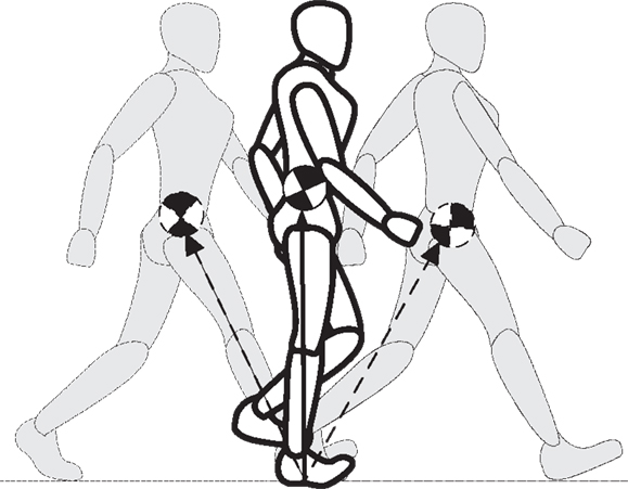
Figure 1. Biomechanical model for human balance and walking as an inverted pendulum.

The ankle joint in the SIP model is assumed to be a two degrees of freedom rotational joint. The CoM is allowed to move in three-dimensional space due to the two rotational degrees of freedom at the ankle. As a result, the CoM can fall anywhere on the surface defined by the hemisphere of radius equal to the stance leg length, as can be seen in Figure 2. This way the constraint to maintain constant height for the CoM off the ground is not required and more natural motion can be generated and controlled.

FIGURE 2

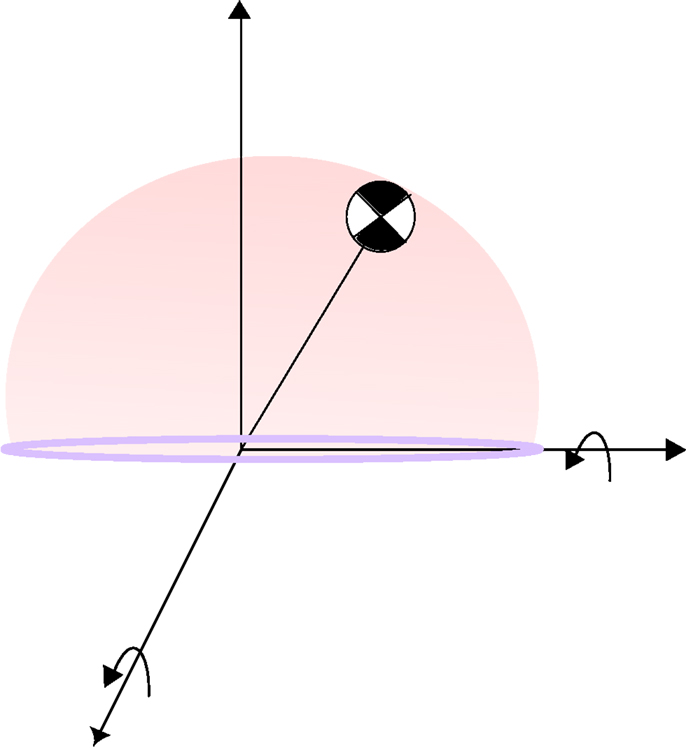
Figure 2. Spherical inverted pendulum with two degrees of freedom at the pivot point.

The CoM location in the local frame of reference is defined by p = (0, l, 0)^T, where l is the length of the fully extended stance leg. The two rotational DoFs represent a rotation around the x and z axes as defined in Figure 2. The world position of the CoM is then given as:

${}^{w}p=\left[\begin{array}{c}\hfill -\mathit{sin}\left(\mathrm{\varphi }\right)\mathit{cos}\left(\mathrm{\theta }\right)l\hfill \\ \hfill \mathit{cos}\left(\mathrm{\varphi }\right)\mathit{cos}\left(\mathrm{\theta }\right)l\hfill \\ \hfill \mathit{sin}\left(\mathrm{\theta }\right)l\hfill \\ \hfill \hfill \end{array}\right]$ (2)

The equations of motion have the following form:

$\frac{d}{\mathit{dt}}\frac{\partial \mathcal{L}}{\partial \dot{q}}+\frac{\partial \mathcal{L}}{\mathit{\partial q}}=\mathrm{\tau }$ (3)

where $\mathcal{L}$ = K – U is the Lagrangian defined as the difference between the kinetic energy, K, and the potential energy, U. The system state variable $q={\left(\mathrm{\theta \hspace{0.17em}\hspace{0.17em}\hspace{0.17em}\varphi }\right)}^T$ is the angles of the ankle joint and τ is a (2 × 1) vector of actuator torques. Carrying out the derivatives in Eq. 3, we derive the dynamic equations of the system as below:

${\mathit{ml}}^2\ddot{\theta }+m{l}^2{\dot{\varphi }}^2\mathit{sin}\left(\mathrm{\theta }\right)\mathit{cos}\left(\mathrm{\theta }\right)-\mathit{mlgcos}\left(\mathrm{\varphi }\right)\mathit{sin}\left(\mathrm{\theta }\right)={\mathrm{\tau }}_{\mathrm{\theta }}$ (4)

$m{l}^2\mathit{cos}{\left(\mathrm{\theta }\right)}^2\ddot{\varphi }-2\dot{\varphi }\dot{\theta }\mathit{tan}\left(\mathrm{\theta }\right)-\frac{\mathit{gsin}\left(\mathrm{\varphi }\right)}{\mathit{lcos}\left(\mathrm{\theta }\right)}={\mathrm{\tau }}_{\mathrm{\varphi }}$ (5)

As can be seen from Eqs 4 and 5, the system is non-linear and there is a degree of cross coupling between the two degrees of freedom appearing in the form of the Centrifugal and Coriolis terms in the equations of motion. In the next section, we will introduce a dissipative energy controller that is able to stabilize the pendulum in its upright posture.

3. SIP Balancing Using Dissipative Control

In order to find a storage function for the SIP model as defined by Willems (2007), we consider only one degree of freedom. Linearizing Eq. 4 around the upright posture, θ = 0, the unpowered system’s equation of motion is given by:

$\ddot{\theta }=\frac{g}{l}\mathrm{\theta }$ (6)

The above system behaves like a spring-mass system with negative stiffness of k = −g/l. A conserved quantity E_SIP can be defined as:

$E_{\mathit{SIP}}=-\frac{1}{2}{\dot{\theta }}^2+\frac{g}{2l}{\mathrm{\theta }}^2$ (7)

The E_SIP represents the sum of the potential and kinetic energies. It can be interpreted as the stored energy function of the one degree of freedom inverted pendulum. The system is stabilized when the quantity E_SIP = 0. The solution to this stable condition results in the eigenvalues of the system as given below:

$\dot{\theta }=\pm \sqrt{\frac{g}{l}}\mathrm{\theta }$ (8)

The solution given by Eq. 8 represents a saddle point in the system dynamics with a stable eigenvector when θ and $\dot{\theta }$ have opposite signs (the CoM is moving toward the pivot point), and unstable eigenvector when the signs are the same (the CoM is moving away from the pivot point). Rearranging Eq. 8, the state-space stability condition, defined as P, is given by:

$P=\mathrm{\theta }+\sqrt{\frac{l}{g}}\dot{\theta }=0$ (9)

However, when the system is disturbed, the above stability condition does not hold and P ≠ 0. Using a standard proportional control law with gain, k_p, with the goal of restoring P to 0, the control input u can be defined as:

$u=-k_{p}P$ (10)

The control input, u, is then related to the ankle joint torque, τ, as follows:

$\mathrm{\tau }=\mathit{mglsin}\left(u\right)$ (11)

Using the control torque as the driving input to the linearized system described by Eq. 6, the system can be represented by:

$\ddot{\theta }=\frac{g}{l}\left(\mathrm{\theta }+u\right)$ (12)

The approximation sin(u) ≈ u was used in simplifying Eq. 12. Substituting the values of u and P from Eqs. 7 and 9, and simplifying, we get the following, where $\mathrm{\omega }=\sqrt{\frac{g}{l}}$

$\ddot{\theta }=\left(1-k_p\right){\mathrm{\omega }}^2\mathrm{\theta }-k_p\mathrm{\omega }\dot{\theta }$ (13)

This controller offers the benefits of ease of tuning in comparison to standard proportional derivative controllers, since there is only one gain variable instead of two tunable gains. Furthermore, we will show in the next section that this controller results in a critically damp response, achieving the fastest stabilization time with the least amount of energy consumption possible.

4. Simulation Results of the SIP Dissipative Energy Controller

To verify the validity of the energy controller described above, we have run a number of simulation experiments, using classical control approaches, such as PD + Gravity compensation, and the Energy controller presented here. The control torque was constrained to ensure that the CoP does not leave the support polygon defined by the foot. Assuming that the foot is fixed to the floor and the ankle torque does not result in slippage or foot rotation, Yu et al. (2009) define the CoP location to be given by

$x_{\mathit{cop}}=\frac{-\mathrm{\tau }}{F_Z}$ (14)

where τ is the total moment generated at the ground contact (the pivot point) of the SIP. The other constraint is due to friction and guarantees that the no slippage assumption is held.

$∥\frac{F_X}{F_Z}∥\le \mathrm{\mu }$ (15)

Where F_X and F_Z are the components of the ground reaction force. From Eq. 15, it is clear that the ground reaction force in the z direction, F_Z, must satisfy the following inequality:

$F_Z\ge ∥\frac{F_X}{\mathrm{\mu }}∥$ (16)

Furthermore, F_Z is expressed as:

$F_Z=m\left({\ddot{x}}_Z+g\right)$ (17)

where ${\ddot{x}}_Z$ is the vertical acceleration of the CoM, m is the system mass, and g is the gravity acceleration. From the constraint of Eq. 16 and the constraint to maintain the CoP within the support polygon defined by the foot, the maximum joint torque that can be generated by the controller is written as a function of the ground reaction force and the support polygon dimensions as follows:

${\mathrm{\tau }}_{\mathit{max}}=\mathit{md}\left({\ddot{x}}_Z+g\right)$ (18)

where d defines the edge of the support polygon. The SIP was subjected to an instantaneous impulse varying in magnitude up to 5 Nm. The objective of the control was to restore the pendulum to a stable upright posture. Table 1 shows the parameters of the humanoid robot used in the simulations. Figure 3 shows the closed-loop system response for the different disturbances. The solid colored lines represent the response of the energy controller, whereas the dotted lines represent the classical controller response. The energy controller response resembles that of a critically damped system resulting in increased stability margins, since it does not suffer from any oscillation and overshoot in the system’s response observed in the hand tuned PD controller.

TABLE 1

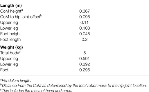
Table 1. Humanoid robot parameters used in the simulations.

FIGURE 3

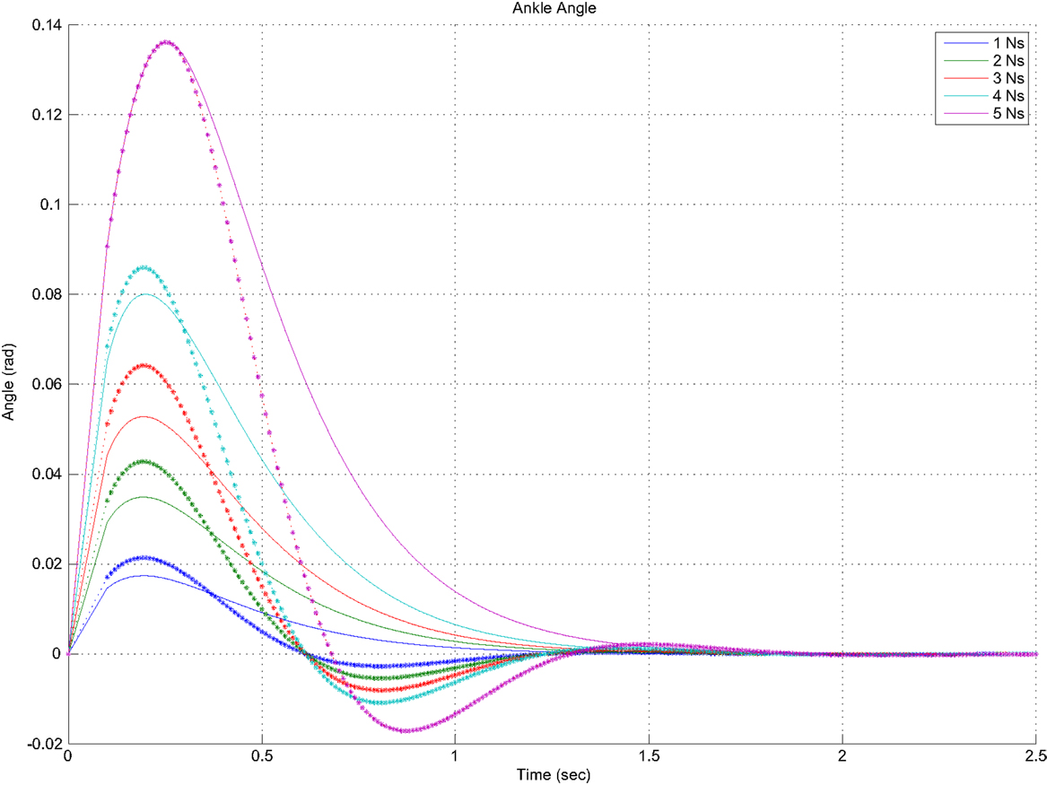
Figure 3. Ankle joint trajectories for a range of disturbance sizes.

The resulting controlling torque from both control approaches is shown in Figure 4. Similarly, the solid lines represent the torque resulting from the energy controller, whereas the dotted lines represent the PD controller torques. The energy controller requires less overall torque to restore balance in response to the impulse disturbances. As a result, it requires less energy in comparison to the PD controller. Furthermore, the critically damped nature of the SIP energy controller ensures that no energy is expended in attenuating the oscillations that result from the undamped PD controller.

FIGURE 4

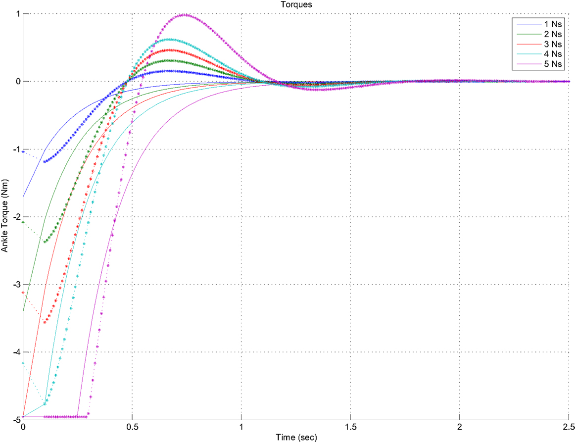
Figure 4. Ankle torques for the same range of perturbation.

From the static kinematic analysis of the inverted pendulum, Flanagan (2014) relates the sway angle to the CoP location during quiet standing by

$x_{\mathit{CoP}}=-\mathit{lsin}\left(\mathrm{\theta }\right)$ (19)

Solving Eq. 19 for θ to derive the largest possible sway angle, we get:

$\mathrm{\theta }=-\mathit{si}{n}^{-1}\left(\frac{x_{\mathit{CoP}}}{l}\right)$ (20)

where l is the length of the stance leg and x_CoP is the location of the center of pressure.

Both controllers manage to stabilize the SIP in face of impulse disturbances with a maximum sway angle of around 8°, which is well within the limits described in Eq. 20 when solved using the parameters of our robot hardware. The limit on the sway angle for the robot hardware was found to be ±17°.

In the case of large disturbances, a different strategy needs to be used to avoid falling over. One such strategy is to allow the robot to take a step in order to enlarge its support polygon and prevent a fall. The optimal stepping location is defined using the concept of the capture point (Pratt et al., 2006). Taking into account the effects of the instantaneous impact of the swing leg, the pendulum angular velocity just before impact is determined by the following:

$\dot{\theta }=\frac{\mathrm{\omega }\mathit{sin}\left(\mathrm{\theta }\right)}{\left(2\mathit{sin}\left(\mathrm{\theta }\right)\mathit{tan}\left(\mathrm{\theta }\right)+\mathit{cos}\left(\mathrm{\theta }\right)\right).\sqrt{\mathit{cos}\left(\mathrm{\theta }\right)}}$ (21)

To compute the required orientation of the robot in terms of its ankle angular velocity $\dot{\theta }$, Eq. 21 is solved numerically and the optimal step location is found to be the intersection point between the CoM trajectory and the resulting trajectory from solving Eq. 21.

For small angular velocities, the biped angle before impact is a linear function of the velocity. A linear approximation can be used to simplify the computation time when implemented on the computer for simulation or on the actual robot hardware. If the angular velocity is larger than ±1 rad/s, the system is forced to take a number of steps before it can reach a complete stop in a balanced state due to size limitation of the biped robot. The exact step length l_s is defined as a function of the ankle angle and the leg length as:

$l_s=2\mathit{lsin}\left(\mathrm{\theta }\right)$

where l is the pendulum length and θ is the angle between the pendulum and the vertical just before taking the step, which was found to be around ±20° in the sagittal plane. The foot landing position in the frontal plane is decided so that the pivot point of the pendulum coincides with the CoM ground projection when the robot comes to a stop. Hence, the pendulum angle ϕ after taken a step is always equal to zero.

4.1. Comparison of Canonical and Energy Controllers

Reducing the required energy to maintain the standing balance will prolong the battery life and autonomous behavior of the humanoid robot. Figure 5 shows the delta in the total mechanical energy of the SIP humanoid robot model in response to small disturbances. It is evident that the new energy controller achieves faster response time in comparison to the canonical control approaches. It is also visible that the energy-based controller requires less overall energy in restoring the system balanced state in comparison to the classical approaches, without the need for extensive tuning of the different gains in the control system.

FIGURE 5

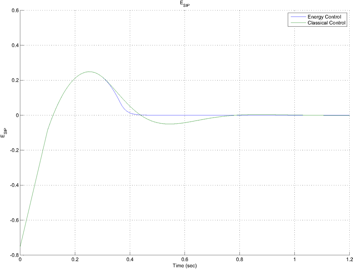
Figure 5. Comparison between the TME change using energy-based controller vs. standard controller.

The transfer function from the measurement noise to the output of the closed-loop energy control law is denoted by T, the complementary sensitivity function

$T_{\mathit{Energy}}=\frac{\mathrm{\omega }{K}_{p}s+{\mathrm{\omega }}^2{K}_p}{s^2+\mathrm{\omega }{K}_{p}s-{\mathrm{\omega }}^2\left(1-K_p\right)}$ (22)

while in the case of the classical PD control the same transfer function is given by:

$T_{\mathit{PD}}=\frac{K_{d}s+K_p}{m{l}^2{s}^2+K_{d}s-\left(\mathit{mlg}-K_p\right)}$ (23)

The energy control law transfer function, T_Energy, depends only on the gain variable, K_P. While T_PD depends on both the proportional and derivative gains as well as the mass of the pendulum. Both Eqs 22 and 23 behave as low-pass filters as shown in the Bode plot of Figure 6. The steady-state (DC) gain of these transfer functions is given by:

$G_{\mathit{ss}}=\underset{s\to 0}{\lim }T\left(s\right)$

FIGURE 6

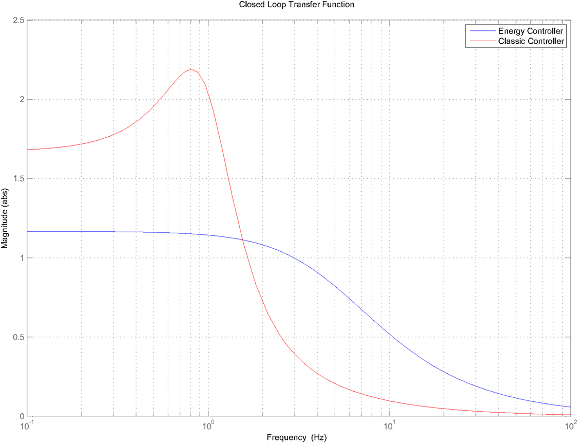
Figure 6. Bode plot of the closed-loop SIP system using both control laws.

For the energy control law, the steady-state gain is defined to be:

$G_{{\mathit{Energy}}_{\mathit{ss}}}=\frac{K_p}{K_p-1}$ (24)

The classical control law has a similar expression for the steady-state gain as that given by Eq. 24. The steady-state gain is given by:

$G_{{\mathit{PD}}_{\mathit{ss}}}=\frac{K_p}{K_p-\mathit{mlg}}$ (25)

For large proportional gains, the steady-state gain of both transfer functions approaches one. In most practical situations, this ideal case cannot be achieved, since the value of these gains is limited to an upper bound. The maximum gain value is imposed by the actuator saturation limits, or in the case of humanoid robots, by the center of pressure constraints. In this situation, the DC gain will be larger than 1, as evident from the denominator of both Eqs 24 and 25.

The magnitude of the transfer function for both systems decays to zero as the frequency increases as shown in Figure 6. The classical control magnitude decays faster than the energy-based controller. However, it is evident from the Bode plot of the PD transfer function that a peak at low frequencies exists. This peak corresponds to the overshoot in the time response when using the PD controller to restore the pendulum to its upright posture. On the other hand, the energy-based controller does not suffer from such effects. In fact, it acts similarly to a critically damped system, as observed in its time response.

To simulate walking at low speeds, the ankle joint of the pendulum is demanded to go back and forth at a rate of two steps per second. A sinusoidal input signal, r(t), was used as the driving input for both systems.

$r\left(t\right)=\mathit{sin}\left(\mathrm{4\pi }t\right)$ (26)

The top graph in Figure 7 shows the tracking response of the two control methods. The classical control system has a large tracking error and phase delay of roughly π/2. On the other hand, the response from the energy controller closely tracks the input signal in terms of the amplitude and the phase of the signal.

FIGURE 7

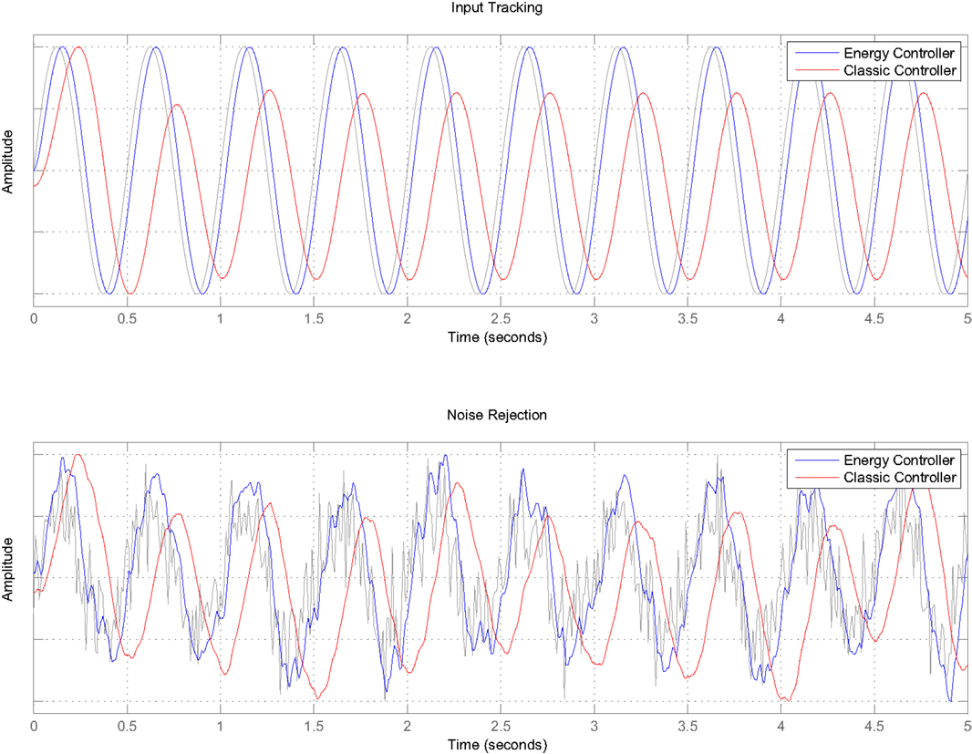
Figure 7. Reference input tracking comparison between the novel energy-based controller and a classical PD + gravity controller.

To simulate the effects of the real-world measurement and actuation noise, white Gaussian noise was added to the input signal before being fed to the system. The noise signal was filtered at 100 Hz to model the bandwidth of our robot hardware joint position and IMU sensors. This is also the sampling frequency at which the control loop will be running on the robot. The bottom graph of Figure 7 shows the response of both controllers. The PD control system performs better in rejecting the high-frequency noise compared to the energy control system. However, this is expected due to the larger bandwidth of the energy-based control law in comparison to the classical method, as can be determined from Figure 6.

On the other hand, the energy-based controller tracks the input signal, r(t), closely as can be seen at the top graph in Figure 7. The PD controller causes a larger phase delay and more attenuation to the input signal of almost 30%.

5. Ankle Strategy Stability Regions

The orbital energy of the SIP model defined by Eq. 7 is a conserved quantity until the moment of touch-down or lift-off of the swing foot. As the CoM moves toward the pivot point, three situations are possible depending on the value of E_SIP

• E_SIP > 0, the CoM will pass the pivot point and carry on in the same direction

• E_SIP < 0, the CoM will come to a stop over the pivot point momentarily before reversing direction and starting to move in the opposite direction

• E_SIP = 0, the CoM will come to a rest over the pivot point, resulting in a stable stance.

The solution to the stable condition is given by Eq. 8. From the center of pressure constraint on the control input to the system, the maximum input torque on the system, assuming ${\ddot{x}}_z=0$, is given by

${\mathrm{\tau }}_{\mathit{max}}=\mathit{mgd}$ (27)

where m is the total mass of the system, g is the acceleration due to gravity, and d is the distance from the pivot point to the edge of the support region. Defining the pendulum angle, δ_θ, as the maximum possible sway angle as defined by Eq. 20, expressing d in terms of δ_θ, Eq. 27 becomes

${\mathrm{\tau }}_{\mathit{max}}=\mathit{mglsin}\left({\mathrm{\delta }}_{\mathrm{\theta }}\right)$ (28)

The maximum acceleration, $\ddot{\theta }$, due to the maximum control torque is then given by

${\ddot{\theta }}_{\mathit{max}}=\frac{g}{l}\mathrm{\theta }-\frac{g}{l}\mathit{sin}\left({\mathrm{\delta }}_{\mathrm{\theta }}\right)$ (29)

By analogy, the saddle point of the system when E_SIP = 0 is expressed as

${\dot{\theta }}_{\mathit{max}}=\pm \sqrt{\frac{g}{l}}\left(\mathrm{\theta }-\mathit{sin}\left({\mathrm{\delta }}_{\mathrm{\theta }}\right)\right)$ (30)

The above equation describes the stability bounds on the SIP while using the ankle balancing strategy. The stable region in terms of the SIP states is then defined as

$\mathit{sin}\left({\mathrm{\delta }}_{\mathrm{\theta }}^{-}\right)<\mathrm{\theta }+\sqrt{\frac{l}{g}}\dot{\theta }<\mathit{sin}\left({\mathrm{\delta }}_{\mathrm{\theta }}^{+}\right)$ (31)

Figure 8 shows that all the stable trajectories in blue fall in the middle section defined by the two yellow lines. The region defined by Eq. 31 and the numerical simulations for balance recovery show that the system is able to recover from a push impulse with a magnitude of 5.7 Ns. The fact that both methods coincide validates our assumptions in deriving the stability bounds, allowing the control framework to monitor the angular state of the SIP to make a decision on the method to be used in recovering and restoring balance to the humanoid robot.

FIGURE 8

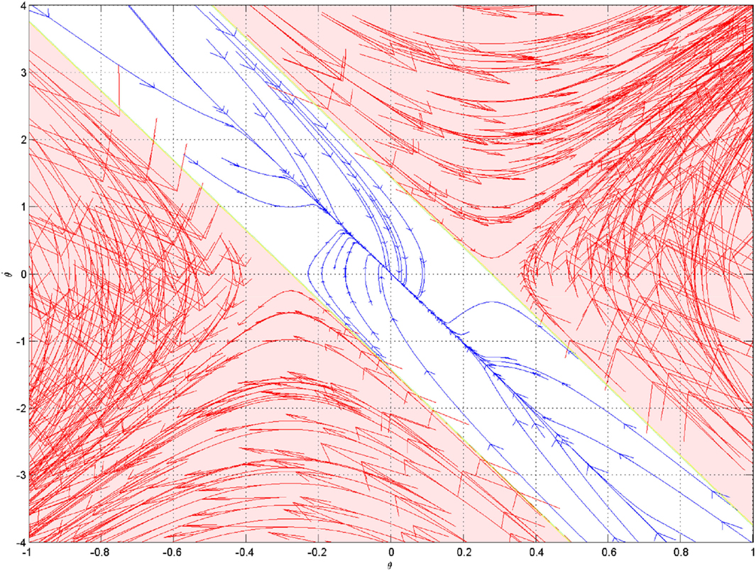
Figure 8. Angular stability regions as defined by the SIP Ankle Balance Strategy.

6. Walking Gait Generation

The SIP model is used to generate and control a stable walking gait using the principles of passive dynamic walking. The SIP model is extended to be described as a hybrid dynamic system with two stages. The first is a continuous dynamic model for the Single Support Phase to describe the CoM behavior. The second stage is during the exchange of support instance and impact of the swing leg. After each impact, an internal impulse push is used to restore any lost energy due to the impact with the ground. In the proposed control architecture, the SIP model and its energy-based control are considered as an internal model that provides the CoM and feet trajectories during the walking cycle. These trajectories are converted to joint motion through a full-body inverse kinematics algorithm to be executed through the robot individual joints. The full control framework is visualized in Figure 9.

FIGURE 9

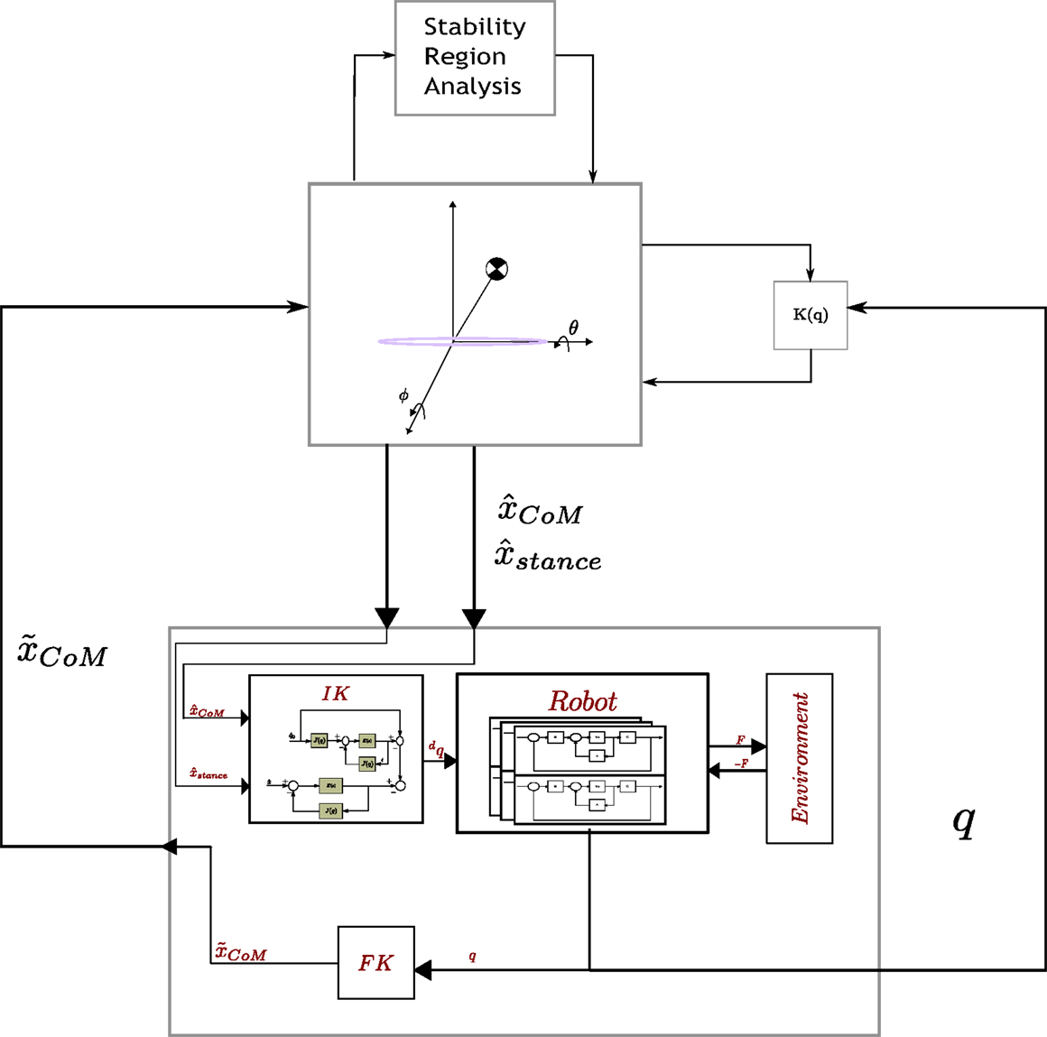
Figure 9. Complete control framework for standing balance and walking gait generation. The diagram shows how the SIP model and the energy-based controllers are used as an internal control loop that provides CoM and foot trajectories to the humanoid robots while receiving the actual CoM and feet location in the feedback loop.

The walk cycle stability is a nominally periodic sequence of steps that is stable as a whole, but not locally stable at every instant in time. The motion stability in this way is defined as “the ability to interrupt and avoid a fall.”

In order to generate a walking gait, the authors extended the stepping strategy for standing balance through the injection of a virtual impulse push into the controller at the moment of impact to restore any energy loss. The energy loss is modeled through the angular velocity loss of the pendulum as described below:

${\dot{\theta }}^{+}=\mathit{lcos}\left(2{\mathrm{\theta }}^{-}\right){\dot{\theta }}^{-}$ (32)

where θ⁻ is the pendulum angle just before impact and θ⁺ is the angle just after impact and l is the pendulum length. Under these conditions, every step of the walking gait is defined as an interrupted fall and the overall motion is stable as a whole, but not locally stable at every instant in time. Hobbelen and Martijn (2007) define this a “limit cycle walking.”

The motion in the frontal place of the robot is controlled in such a way that will translate the CoM from side to side during the walk. This motion trajectory is dependent on the CoM trajectory in the sagittal plane. This trajectory is provided as a reference input to the energy controller for the CoM motion to follow. Figure 10 shows the projection of the CoM motion on the ground along with the step locations.

FIGURE 10

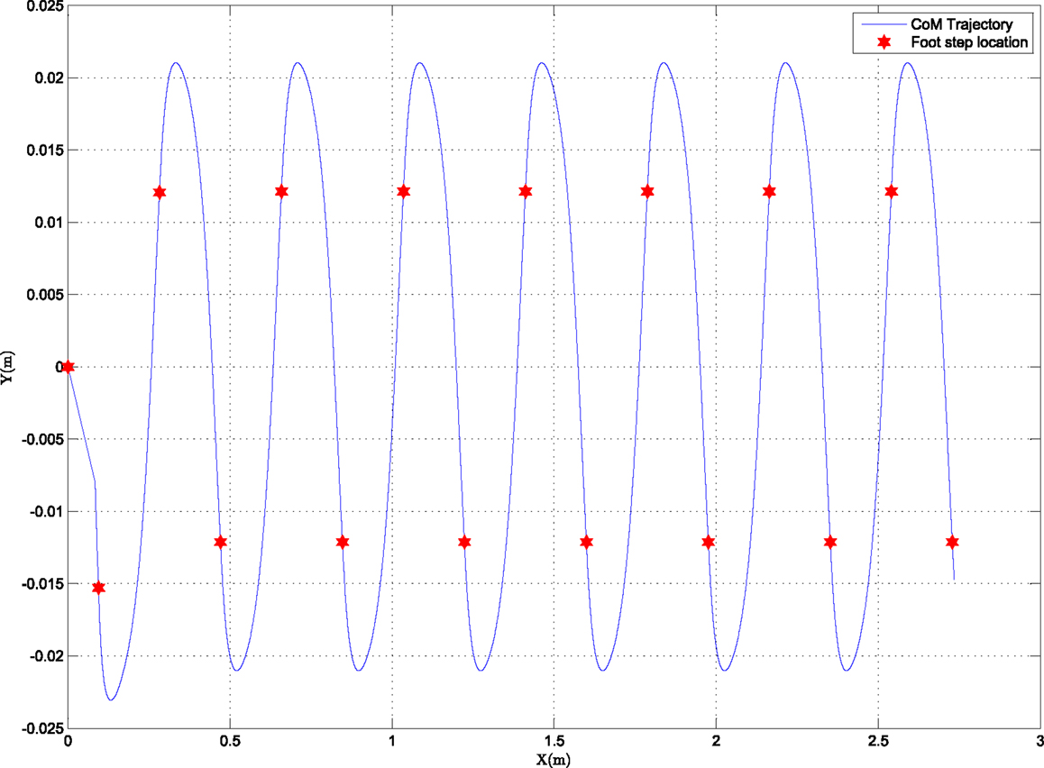
Figure 10. Top view of the CoM motion as a result of the simulation of the gait generation and control method for a number of steps. The foot locations are also shown highlighting the support exchange from one foot to the next.

The resulting CoM trajectory is shown in Figure 11. By comparison to the findings of the CoM motion characterized by biomechanical researchers shown in Figure 12, we can see large similarities between the two trajectories. The shape and phase of the forward direction resembles two sinusoidal curves. The maxima occur at about ∼35% and ∼85% of the gait cycle, whereas the minima occur at the moment of foot impact at ∼10% and ∼60% of the cycle. On the other hand, the lateral displacement is represented with a sinusoidal curve, ensuring the CoM is moved from one support foot to the other. The phase difference between the SIP and biomechanical trajectory is resulting from the first step choice, and it does not change the nature of the results.

FIGURE 11

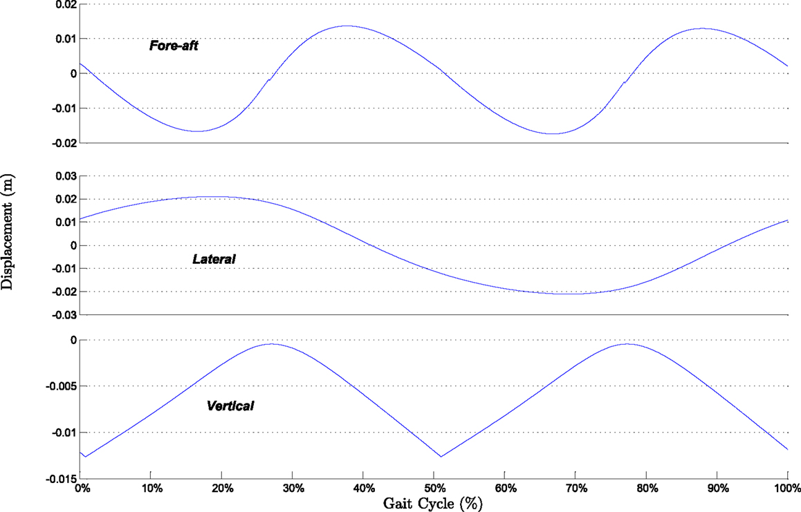
Figure 11. CoM displacement as a result of the gait generation approach developed using the SIP control framework.

FIGURE 12

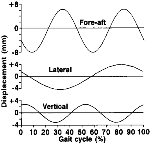
Figure 12. Biomechanics measurements of CoM displacement (Whittle, 1997).

The vertical motion has the same periodicity as that of the human walk. However, the SIP-generated trajectory has an instantaneous change in the direction of the CoM motion at the moment of foot impact at ∼50% of the gait cycle. This instantaneous change results from the stepping model used with the SIP biped model. The CoM reaches its highest point twice during the gait cycle at around 25 and 75% of the cycle. This is the time when the support leg is fully extended and is in an upright position. The lowest CoM position occurs at the moment of switching support. Figure 13 shows a series of screenshots of the resulting walking motion. It should be noted here that the entire motion was generated using the SIP CoM trajectories and a fifth-order polynomial to give the swing foot trajectory. The difference between this approach and that of the standard 3DLIPM approaches can be summarized by the fact that the motion of the CoM is not constrained to a constant height of the plane during a single-step motion resulting in a more natural overall motion for the entire humanoid body.

FIGURE 13

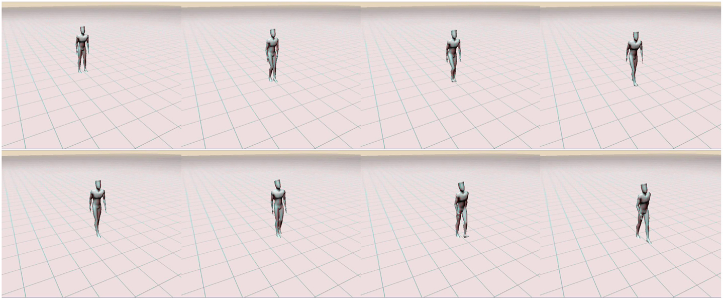
Figure 13. Screenshots of the generated full-body walking motion as a result of the proposed approach.

7. Conclusion

This article presents the Spherical Inverted Pendulum model for the biped standing balance control. It describes the system using the two rotational degrees of freedom at the ankle and does not suffer from the limiting assumptions of the traditional approaches such as maintaining a constant CoM height off the ground.

We also described an energy-based control architecture for push recovery on humanoid robots. This control method transforms the SIP model into a critically damped system with the use of a single tuning parameter, so that balance is restored in the fastest and most energy efficient way possible. Finally, a description of the stability bounds and walking gait generation method using the SIP and the energy controller is presented.

Author Contributions

AE developed the SIP model and the passivity-based control law and performed the simulations under AP’s direct supervision throughout the research process. AE wrote the manuscript. AP provided editing comments. AP was AE’s first supervisor during his studies.

Conflict of Interest Statement

The authors declare that the research was conducted in the absence of any commercial or financial relationships that could be construed as a potential conflict of interest.

Funding

This research has been partly funded by the Libyan Higher Education Ministry.

References

Atkeson, C. G., and Stephens, B. (2007). “Multiple balance strategies from one optimization criterion,” in 2007 7th IEEE-RAS. International Conference on Humanoid Robots (Pittsburgh, PA: Institute of Electrical Engineers, IEEE), 57–64

Google Scholar

Flanagan, S. P. (2014). “Chapter explaining motion II: angular kinematics,” in Biomechanics: A Case-Based Approach, ed. M. R. Turner (Burlington, MA: Jones & Bartlett Publishers), 120.

Google Scholar

Fujimoto, Y., and Kawamura, A. (1998). Simulation of an autonomous biped walking robot including environmental force interaction. IEEE Robot. Autom. Mag. 5, 33–42. doi:10.1109/100.692339

CrossRef Full Text | Google Scholar

Hashimoto, K., Takezaki, Y., Lim, H.-O., and Takanishi, A. (2013). Walking stabilization based on gait analysis for biped humanoid robot. Adv. Robot. 27, 541–551. doi:10.1080/01691864.2013.777015

CrossRef Full Text | Google Scholar

Hirai, K., Hirose, M., Haikawa, Y., and Takenaka, T. (1998). “The development of honda humanoid robot,” in IEEE International Conference on Robotics and Automation (Leuven: Institute of Electrical Engineers, IEEE), 1321–1326.

Google Scholar

Hobbelen, D. G. E., and Martijn, W. (2007). “Limit cycle walking,” in Humanoid Robots: Human-Like Machines, ed. M. Hackel (Vienna: I-Tech), 642.

Google Scholar

Horak, F. B., and Nashner, L. M. (1986). Central programming of postural movements: adaptation to altered support-surface configurations. J. Neurophysiol. 55, 1369–1381.

PubMed Abstract | Google Scholar

Kajita, S., Kanehiro, F., Kaneko, K., Fujiwara, K., Harada, K., Yokoi, K., et al. (2003). “Biped walking pattern generation by using preview control of zero-moment point,” in Robotics and Automation, 2003. Proceedings. ICRA ’03. IEEE International Conference on, Vol. 2 (Taipei: Institute of Electrical Engineers, IEEE), 1620–1626.

Google Scholar

Kajita, S., Kanehiro, F., Kaneko, K., Yokoi, K., and Hirukawa, H. (2001). “The 3d linear inverted pendulum mode: a simple modeling for a biped walking pattern generation,” in Intelligent Robots and Systems, 2001. Proceedings. 2001 IEEE/RSJ International Conference on, Vol. 1 (Maui: Institute of Electrical Engineers, IEEE), 239–246.

Google Scholar

Kajita, S., and Tanie, K. (1991). “Study of dynamic biped locomotion on rugged terrain – derivation and application of the linear inverted pendulum mode,” in Robotics and Automation, 1991. Proceedings. 1991 IEEE International Conference on, Vol. 2 (Sacramento, CA: Institute of Electrical Engineers, IEEE), 1405–1411.

Google Scholar

Maki, B. E., and McIlroy, W. E. (1997). The role of limb movements in maintaining upright stance: the “change-in-support” strategy. Phys. Ther. 77, 488–507.

PubMed Abstract | Google Scholar

Nishiwaki, K., and Kagami, S. (2007). “Walking control on uneven terrain with short cycle pattern generation,” in Humanoid Robots, 2007 7th IEEE-RAS International Conference on, 447–453.

Google Scholar

Pratt, J., Carff, J., Drakunov, S., and Goswami, A. (2006). “Capture point: a step toward humanoid push recovery,” in Humanoid Robots, 2006 6th IEEE-RAS International Conference on, (Genova: Institute of Electrical Engineers, IEEE), 200–207.

Google Scholar

Stephens, B. (2007). “Humanoid push recovery,” in IEEE-RAS International Conference on Humanoid Robots. Pittsburgh, PA: Institute of Electrical Engineers, IEEE.

Google Scholar

Sugihara, T., and Nakamura, Y. (2003). “Whole-body cooperative COG control through ZMP manipulation for humanoid robots,” in 2nd International Symposium on Adaptive Motion of Animals and Machines (AMAM2003).

Google Scholar

Sugihara, T., Nakamura, Y., and Inoue, H. (2002). “Real-time humanoid motion generation through ZMP manipulation based on inverted pendulum control,” in IEEE International Conference on Robotics and Automation, Vol. 2. Washington, DC.

Google Scholar

Uyar, E., Baser, Ö., Baci, R., and Özçivici, E. (2009). Investigation of Bipedal Human Gait Dynamics and Knee Motion Control. Technical Report. Izmir: Department of Mechanical Engineering, Faculty of Engineering, Dokuz Eylül University.

Google Scholar

Wang, B., Hu, R., Zhang, J., and Huai, C. (2009). Balance recovery control for biped robot based on reaction null space method. J. Control Theory Appl. 7, 87–91. doi:10.1007/s11768-009-7019-4

CrossRef Full Text | Google Scholar

Whittle, M. W. (1997). Three-dimensional motion of the center of gravity of the body during walking. Hum. Mov. Sci. 16, 347–355. doi:10.1016/S0167-9457(96)00052-8

CrossRef Full Text | Google Scholar

Willems, J. (2007). Dissipative dynamical systems. Eur. J. Control 13, 134–151. doi:10.3166/ejc.13.134-151

CrossRef Full Text | Google Scholar

Winter, D. A. (1995). Human balance and posture control during standing and walking. Gait Posture 3, 193–214. doi:10.1016/0966-6362(96)82849-9

CrossRef Full Text | Google Scholar

Yu, W., Bao, G., and Wang, Z. (2009). “Effects of joint torque constraints on humanoid robot balance recovery in the presence of external disturbance,” in Robotics and Biomimetics (ROBIO), 2009 IEEE International Conference on (Guilin: Institute of Electrical Engineers, IEEE), 2361–2367.

Google Scholar