Bounded Rationality, Abstraction, and Hierarchical Decision-Making: An Information-Theoretic Optimality Principle

1. Introduction

A key characteristic of intelligent systems, both biological and artificial, is the ability to flexibly adapt behavior in order to interact with the environment in a way that is beneficial to the system. In biological systems, the ability to adapt affects the fitness of an organism and becomes key to survival not only of individual organisms but species as a whole. Both in the theoretical study of biological systems and in the design of artificial intelligent systems, the central goal is to understand adaptive behavior formally. A formal framework for tackling the problem of general adaptive systems is decision-theory, where behavior is conceptualized as a series of optimal decisions or actions that a system performs in order to respond to changes to the input of the system. An important idea, originating from the foundations of decision-theory, is the maximum expected utility (MEU) principle (Ramsey, 1931; Von Neumann and Morgenstern, 1944; Savage, 1954). Following MEU, an intelligent system is formalized as a decision-maker that chooses actions in order to maximize the desirability of the expected outcome of the action, where the desirability of an outcome is quantified by a utility function.

A fundamental problem of MEU is that the computation of an optimal action can easily exceed the computational capacity of a system. It is for example in general prohibitive trying to compute an optimal chess move due to the large number of possibilities. One way to deal with such problems is to study optimal decision-making with information-processing constraints. Following the pioneering work of Simon (1955, 1972) on bounded rationality, decision-making with limited information-processing resources has been studied extensively in psychology (Gigerenzer and Todd, 1999; Camerer, 2003; Gigerenzer and Brighton, 2009), economics (McKelvey and Palfrey, 1995; Rubinstein, 1998; Kahneman, 2003; Parkes and Wellman, 2015), political science (Jones, 2003), industrial organization (Spiegler, 2011), cognitive science (Howes et al., 2009; Janssen et al., 2011), computer science, and artificial intelligence research (Horvitz, 1988; Lipman, 1995; Russell, 1995; Russell and Subramanian, 1995; Russell and Norvig, 2002; Lewis et al., 2014). Conceptually, the approaches differ widely ranging from heuristics (Tversky and Kahneman, 1974; Gigerenzer and Todd, 1999; Gigerenzer and Brighton, 2009; Burns et al., 2013) to approximate statistical inference schemes (Levy et al., 2009; Vul et al., 2009, 2014; Sanborn et al., 2010; Tenenbaum et al., 2011; Fox and Roberts, 2012; Lieder et al., 2012).

In this study, we use an information-theoretic model of bounded rational decision-making (Braun et al., 2011; Ortega and Braun, 2012, 2013; Braun and Ortega, 2014; Ortega and Braun, 2014; Ortega et al., 2014) that has precursors in the economic literature (McKelvey and Palfrey, 1995; Mattsson and Weibull, 2002; Sims, 2003, 2005, 2006, 2010; Wolpert, 2006) and that is closely related to recent advances in the information theory of perception-action systems (Todorov, 2007, 2009; Still, 2009; Friston, 2010; Peters et al., 2010; Tishby and Polani, 2011; Daniel et al., 2012, 2013; Kappen et al., 2012; Rawlik et al., 2012; Rubin et al., 2012; Neymotin et al., 2013; Tkačik and Bialek, 2014; Palmer et al., 2015). The basis of this approach is formalized by a free energy principle that trades off expected utility, and the cost of computation that is required to adapt the system accordingly in order to achieve high utility. Here, we consider an extension of this framework to systems with multiple information-processing nodes and in particular discuss the formation of information-processing hierarchies, where different levels in the hierarchy represent different levels of abstraction. The basic intuition is that information-processing nodes with little computational resources can adapt only a little for different inputs and are therefore forced to treat different inputs in the same or a similar way, that is the system has to abstract (Genewein and Braun, 2013). Importantly, abstractions arising in decision-making hierarchies are a core feature of intelligence (Kemp et al., 2007; Braun et al., 2010a,b; Gershman and Niv, 2010; Tenenbaum et al., 2011) and constitute the basis for flexible behavior.

The paper is structured as follows. In Section 2, we recapitulate the information-theoretic framework for decision-making and show its fundamental connection to a well-known trade-off in information theory (the rate-distortion problem for lossy compression). In Section 3, we show how the extension of the basic trade-off principle leads to a theoretically grounded design principle that describes how perception is shaped by action. In Section 4, we apply the basic trade-off between expected utility and computational cost to a two-level hierarchy and show how this leads to emergent, bounded-optimal hierarchical decision-making systems. In Section 5, we present a mathematically unifying formulation that provides a starting point for generalizing the principles presented in this paper to more complex architectures.

2. Bounded Rational Decision-Making

2.1 A Free Energy Principle for Bounded Rationality

In a decision-making task with context, an actor or agent is presented with a world-state w and is then faced with finding an optimal action $a_w^{\ast }$ out of a set of actions $\mathcal{A}$ in order to maximize the utility U(w, a):

$a_w^{\ast }=\underset{a}{\arg \max }U\left(w,a\right).$ (1)

If the cardinality of the action-set is large, the search for the single best action can become computationally very costly. For an agent with limited computational resources that has to react within a certain time-limit, the search problem can potentially become infeasible. In contrast, biological agents, such as animals and humans, are constantly confronted with picking an action out of a very large set of possible actions. For instance, when planning a movement trajectory for grasping a certain object with a biological arm with many degrees of freedom, the number of possible trajectories is infinite. Yet, humans are able to quickly find a trajectory that is not necessarily optimal but good enough. The paradigm of picking a good enough solution that is actually computable has been termed bounded rational acting (Simon, 1955, 1972; Horvitz, 1988; Horvitz et al., 1989; Horvitz and Zilberstein, 2001). Note that bounded rational policies are in general stochastic and thus expressed as a probability distribution over actions given a world-state p(a|w).

We follow the work of Ortega and Braun (2013), where the authors present a mathematical framework for bounded rational decision-making that takes into account computational limitations. Formally, an agent’s initial behavior (or search strategy through action-space) is described by a prior distribution p₀(a). The agent transforms its behavior to a posterior p(a|w) in order to maximize expected utility Σ_ap(a|w)U(w, a) under this posterior policy. The computational cost of this transformation is measured by the KL-divergence between prior and posterior and is upper-bounded in case of a bounded rational actor. Decision-making with limited computational resources can then be formalized with the following constrained optimization problem:

$\begin{array}{l}{p}^{\ast }\left(a|w\right)=\underset{p\left(a|w\right)}{\arg \max }{\displaystyle \sum _{a}p\left(a|w\right)U\left(w,a\right)}\text{s.t.}{D}_{\text{KL}}\left(p\left(a|w\right)\left|\right|p_0\left(a\right)\right)\le K.\end{array}$ (2)

This principle models bounded rational actors that initially follow a prior policy p₀(a) and then use information about the world-state w to adapt their behavior to p(a|w) in a way that optimally trades off the expected gain in utility against the transformation costs for adapting from p₀(a) to p(a|w). The constrained optimization problem in equation (2) can be rewritten as an unconstrained variational problem using the method of Lagrange multipliers:

$p^{\ast }\left(a|w\right)=\underset{p\left(a|w\right)}{\arg \max }\underset{{\mathbf{\text{E}}}_{p\left(a|w\right)}\left[U\left(w,a\right)\right]}{\underbrace{{\displaystyle \sum _{a}p\left(a|w\right)U\left(w,a\right)}}}-\frac{1}{\mathrm{\beta }}{\displaystyle \underset{D_{\text{KL}}\left(p\left(a|w\right)\left|\right|p_0\left(a\right)\right)}{\underbrace{\sum _{a}p\left(a|w\right)\log \frac{p\left(a|w\right)}{p_0\left(a\right)}}}},$ (3)

where β is known as the inverse temperature. The inverse temperature acts as a conversion-factor, translating the amount of information imposed by the transformation (usually measured in nats or bits) into a cost with the same units as the expected utility (utils). The distribution p^⋆(a|w) that maximizes the variational principle is given by

$p^{\ast }\left(a|w\right)=\frac{1}{Z\left(w\right)}{p}_0\left(a\right)e^{\mathrm{\beta }U\left(w,a\right)},$ (4)

with partition sum Z(w) = Σ_a p₀(a) e^βU(w,a). Evaluating equation (3) with the maximizing distribution p^⋆(a|w) yields the free energy difference

$\begin{array}{l}\hfill \mathrm{\Delta }F\left(w\right)=\underset{p\left(a|w\right)}{\text{max}}{\mathbf{\text{E}}}_{p\left(a|w\right)}\left[U\left(w,a\right)\right]-\frac{1}{\mathrm{\beta }}{D}_{\text{KL}}\left(p\left(a|w\right)\left|\right|p_0\left(a\right)\right)=\frac{1}{\mathrm{\beta }}\log Z\left(w\right),\end{array}$ (5)

which is well known in thermodynamics and quantifies the energy of a system that can be converted to work. ΔF(w) is composed of the expected utility under the posterior policy p^⋆(a|w) minus information processing cost that is required for computing the posterior policy measured as the Kullback-Leibler (KL) divergence between the posterior p^⋆(a|w) and the prior p₀(a).

The inverse temperature β governs the influence of the transformation cost and thus the boundedness of the actor which determines the maximally allowed deviation of the final behavior p^⋆(a|w) from the initial behavior p₀(a). A perfectly rational actor that maximizes its utility can be recovered as the limit case β → ∞where transformation cost is ignored. This case is identical to equation (1) and simply reflects maximum utility action selection, which is the foundation of most modern decision-making frameworks. Note that the optimal policy p^⋆(a|w) in this case collapses to a delta over the best action $p^{\ast }\left(a|w\right)={\mathrm{\delta }}_{a{a}_w^{\ast }}$. In contrast, β → 0 corresponds to an actor that has infinite transformation cost or no computational resources and thus sticks with its prior policy p₀(a). An illustrative example is given in Figure 1.

FIGURE 1

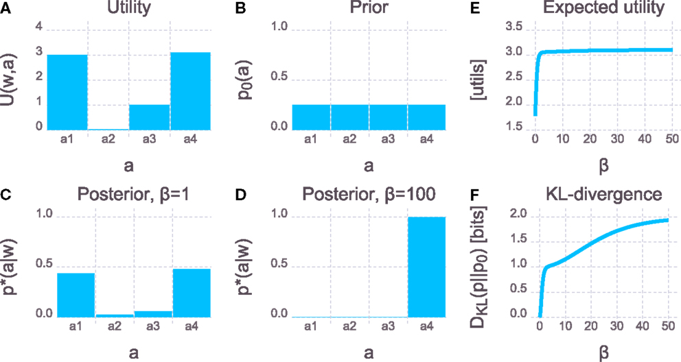
Figure 1. Bounded rationality and the free energy principle. Imagine an actor that has to grasp a particular cup w from a table. There are four options a1 to a4 to perform the movement and the utility U(w, a) shown in (A) measures the performance of each option. There are two actions a1 and a4 that lead to a successful grasp without spilling, and a4 is minimally better. Action a3 leads to a successful grasp but spills half the cup, and a2 represents an unsuccessful grasp. (B) Prior distribution over actions p₀(a): no preference for a particular action. (C) Posterior p*(a|w) [equation (4)] for an actor with limited computational capacity. Due to the computational limits, the posterior cannot deviate from the prior arbitrarily far, otherwise the KL-divergence constraint would be violated. The computational resources are mostly spent on increasing the chance of picking one of the two successful options and decreasing the chance of picking a2 or a3. The agent is almost indifferent between the two successful options a1 and a4. (D) Posterior for an actor with large computational resources. Even though a4 is only slightly better than a1, the agent is almost unbounded and can deviate a lot from the prior. This solution is already close to the deterministic maximum expected utility solution and incurs a large KL-divergence from prior to posterior. (E) Expected utility E_p*(a|w)[U(w, a)] as a function of the inverse temperature β. Initially, allowing for more computational resources leads to a rapid increase in expected utility. However, this trend quickly flattens out into a regime where small increases in expected utility imply large increases in β. (F) KL-divergence D_KL (p*(a|w)||p₀(a)) as a function of the inverse temperature β. In order to achieve an expected utility of ≈ 95% of the maximum utility roughly 1 bit suffices [leading to a posterior similar to (C)]. Further increasing the performance by 5% requires twice the computational capacity of 2 bits [leading to a posterior similar to (D)]. A bounded rational agent that performs reasonably well could thus be designed at half the cost (in terms of computational capacity) compared to a fully rational maximum expected utility agent. An interactive version of this plot where β can be freely changed is provided in the Supplementary Jupyter Notebook “1-FreeEnergyForBoundedRationalDecisionMaking.”

Interestingly, the free energy principle for bounded rational acting can also be used for inference problems. In particular if the utility is chosen as a log-likelihood function U(w, a) = log q(w|a) and the inverse temperature β is set to one, Bayes’ rule is recovered as the optimal bounded rational solution [by plugging into equation (4)]:

$p^{\ast }\left(a|w\right)=\frac{p_0\left(a\right)q\left(w|a\right)}{{\sum }_a{p}_0\left(a\right)q\left(w|a\right)}.$

Importantly, the inverse temperature β can also be interpreted in terms of computational or sample complexity (Braun and Ortega, 2014; Ortega and Braun, 2014; Ortega et al., 2014). The basic idea is that in order to make a decision, the bounded rational decision-maker needs to generate a sample from the posterior p^⋆(a|w). Assuming that the decision-maker can draw samples from the prior p₀(a), samples from the posterior p^⋆(a|w) can be generated by rejecting any samples from p₀(a) until one sample is accepted as a sample of p^⋆(a|w) according to the acceptance rule u ≤ exp(β(U(w, a) − T(w))), where u is drawn from the uniform distribution over the unit interval [0;1] and T(w) is the aspiration level or acceptance target value with T(w) ≥ max_aU(w, a). This is known as rejection sampling (Neal, 2003; Bishop, 2006). The efficiency of the rejection sampling process depends on how many samples are needed on average from p₀(a) to obtain one sample from p^⋆(a|w). This average number of samples $\overline{\mathit{\#Samples}}\left(w\right)$ is given by the mean of a geometric distribution

$\begin{array}{l}\hfill \overline{\mathit{\#Samples}}\left(w\right)=\frac{1}{{\sum }_a{p}_0\left(a\right)\exp \left(\mathrm{\beta }\left(U\left(w,a\right)-T\left(w\right)\right)\right)}=\frac{\exp \left(\mathrm{\beta }T\left(w\right)\right)}{Z\left(w\right)},\end{array}$ (6)

where the partition sum Z(w) is defined as in equation (4). The average number of samples increases exponentially with increasing resource parameter β when T(w) > max_aU(w, a). It is also noteworthy that the exponential of the Kullback-Leibler divergence provides a lower bound for the required number of samples that is $\overline{\mathit{\#Samples}}\left(w\right)\ge \exp \left(D_{\text{KL}}\left(p^{\ast }\left(a|w\right)\left|\right|p_0\left(a\right)\right)\right)$ (see Section 6 in the Supplementary Methods for a derivation). Accordingly, a decision-maker with high β can manage high sampling complexity, whereas a decision-maker with low β can only process a few samples.

2.2 From Free Energy to Rate-Distortion: The Optimal Prior

In the free energy principle in equation (3), the prior p₀(a) is assumed to be given. A very interesting question is which prior distribution p₀(a) maximizes the free energy difference ΔF(w) for all world-states w on average (assuming that p(w) is given). To formalize this question, we extend the variational principle in equation (3) by taking the expectation over w and the arg max over p₀(a)

$\begin{array}{l}\underset{p_0\left(a\right)}{\arg \max }{\displaystyle \sum _{w}p\left(w\right)}\times \left[\underset{p\left(a\left|w\right.\right)}{\arg \max }{\mathbf{\text{E}}}_{p\left(a\left|w\right.\right)}\left[U\left(w,a\right)\right]-\frac{1}{\mathrm{\beta }}{D}_{\text{KL}}\left(p\left(a\left|w\right.\right)∥p_0\left(a\right)\right)\right].\end{array}$

The inner arg max-operator over p(a|w) and the expectation over w can be swapped because the variation is not over p(w). With the KL-term expanded this leads to

$\begin{array}{l}\underset{p_0\left(a\right),p\left(a\left|w\right.\right)}{\arg \max }{\displaystyle \sum _{w,a}p\left(w,a\right)U\left(w,a\right)}-\frac{1}{\mathrm{\beta }}{\displaystyle \sum _{w}p\left(w\right)}{\displaystyle \sum _{a}p\left(a\left|w\right.\right)\log \frac{p\left(a\left|w\right.\right)}{p_0\left(a\right)}}.\end{array}$

The solution to the arg max over p₀(a) is given by $p_0^{\ast }\left(a\right)={\sum }_{w}p\left(w\right)p\left(a|w\right)=p\left(a\right)$. [see Section 2.1.1 in Tishby et al. (1999) or Csiszár and Tusnády (1984)]. Plugging in the marginal p(a) as the optimal prior $p_0^{\ast }\left(a\right)$ yields the following variational principle for bounded rational decision-making

$\begin{array}{l}\underset{p\left(a|w\right)}{\arg \max }\underset{{\mathbf{\text{E}}}_{p\left(a|w\right)}\left[U\left(w,a\right)\right]}{\underbrace{{\displaystyle \sum _{w,a}p\left(w,a\right)U\left(w,a\right)}}}-\frac{1}{\mathrm{\beta }}\underset{I\left(W;A\right)}{\underbrace{{\displaystyle \sum _{w}p\left(w\right)D_{\text{KL}}\left(p\left(a\left|w\right.\right)∥p\left(a\right)\right)}}}=\underset{p\left(a|w\right)}{\arg \max }{J}_{\text{RD}}\left(p\left(a\left|w\right.\right)\right),\end{array}$ (7)

where I(W; A) is the mutual information between actions A and world-states W. The mutual information I(W; A) is a measure of the reduction in uncertainty about the action a after having observed w or vice versa since the mutual information is symmetric

$I\left(W;A\right)=H\left(W\right)-H\left(W|A\right)=H\left(A\right)-H\left(A|W\right)=I\left(A;W\right),$

where H(L) = −Σ_lp(l)log p(l) is the Shannon entropy of random variable L.

The exact same variational problem can also be obtained as the Langragian for maximizing expected utility with an upper bound on the mutual information

$p^{\ast }\left(a|w\right)=\underset{p\left(a|w\right)}{\arg \max }{\displaystyle \sum _{w,a}p\left(w,a\right)U\left(w,a\right)}\text{s.t.}I\left(W;A\right)\le R$ (8)

or in the dual point of view, as minimizing the mutual information between actions and world-states with a lower bound on the expected utility. Thus, the problem in equation (7) is equivalent to the problem formulation in rate-distortion theory (Shannon, 1948; Cover and Thomas, 1991; Tishby et al., 1999; Yeung, 2008), the information-theoretic framework for lossy compression. It deals with the problem that a stream of information must be transmitted over a channel that does not have sufficient capacity to transmit all incoming information – therefore some of the incoming information must be discarded. In rate-distortion theory, the distortion d(w, a) quantifies the recovery error of the output symbol a with respect to the input symbol w. Distortion corresponds to a negative utility which thus leads to an arg min instead of an arg max and a positive sign for the mutual information term in the optimization problem. In this case, a maximum expected utility decision-maker would minimize the expected distortion which is typically achieved by a one-to-one mapping between w and a, which implies that the compression is not lossy. From this, it becomes obvious why MEU decision-making might be problematic: if the MEU decision-maker requires a rate of information processing that is above channel capacity, it simply cannot be realized with the given system.

The solution that extremizes the variational problem of equation (7) is given by the self-consistent equations [see Tishby et al. (1999)]

$\begin{array}{ll}\hfill p^{\ast }\left(a|w\right)& =\frac{1}{Z\left(w\right)}p\left(a\right)e^{\mathrm{\beta }U\left(w,a\right)},\end{array}$ (9)

$\begin{array}{ll}\hfill p\left(a\right)& ={\displaystyle \sum _{w}p\left(w\right)p^{\ast }\left(a|w\right),}\end{array}$ (10)

with partition sum Z(w) = Σ_ap(a)e^βU(w,a).

In the limit case β → ∞where transformation costs are ignored, $p^{\ast }\left(a|w\right)={\mathrm{\delta }}_{a{a}_w^{\ast }}$is the perfectly rational policy for each value of w independent of any of the other policies and p(a) becomes a mixture of these solutions. Importantly, due to the low price of information processing $\frac{1}{\mathrm{\beta }}$, high values of the mutual information term in equation (7) will not lead to a penalization, which means that actions a can be very informative about the world-state w. The behavior of an actor with infinite computational resources will thus in general be very world-state-specific.

In the case where β → 0 the mutual information between actions and world-states is minimized to I(W; A) = 0, leading to p*(a|w) = p(a) ∀w, the maximal abstraction where all w elicit the same response. Within this limitation, the actor will, however, emit actions that maximize the expected utility Σ_{w, a}p(w)p(a) U(w, a) using the same policy for all world-states.

For values of the rationality parameter β in between these limit cases, that is 0 < β < ∞, the bounded rational actor trades off world-state-specific actions that lead to a higher expected utility for particular world-states (at the cost of an increased information processing rate), against more robust or abstract actions that yield a “good” expected utility for many world-states (which allows for a decreased information processing rate).

Note that the solution for the conditional distribution p^⋆(a|w) in the rate-distortion problem [equation (9)] is the same as the solution in the free energy case of the previous section [equation (4)], except that the prior p₀(a) is now defined as the marginal distribution p₀(a) = p(a) [see equation (10)]. This particular prior distribution minimizes the average relative entropy between p(a|w) and p(a) which is the mutual information between actions and world-states I(W; A).

An alternative interpretation is that the decision-maker is a channel that transmits information from w to a according to p(a|w). The channel has a limited capacity, which could arise from the agent not having a “brain” that is powerful enough, but a limited channel capacity could also arise from noise that is induced into the channel, i.e., an agent with noisy sensors or actuators. For a large capacity, the transmission is not severely influenced and the best action for a particular world-state can be chosen. For smaller capacities, however, some information must be discarded and robust (or abstract) actions that are “good” under a number of world-states must be chosen. This is possible by lowering β until the required rate I(W; A) does no longer exceed the channel capacity. The notion that a decision-maker can be considered as an information processing channel is not new and goes back to the cybernetics movement (Ashby, 1956; Wiener, 1961). Other recent applications of rate-distortion theory to decision-making problems can be found for example in Sims (2003, 2006) and Tishby and Polani (2011).

2.3 Computing the Self-Consistent Solution

The self-consistent solutions that maximize the variational principle in equation (7) can be computed by starting with an initial distribution p_init(a) and then iterating equations (9) and (10) in an alternating fashion. This procedure is well known in the rate-distortion framework as a Blahut-Arimoto-type algorithm (Arimoto, 1972; Blahut, 1972; Yeung, 2008). The iteration is guaranteed to converge to a unique maximum [see Section 2.1.1 in Tishby et al. (1999) and Csiszár and Tusnády (1984) and Cover and Thomas (1991)]. Note that p_init(a) has to have the same support as p(a). Implemented in a straightforward manner, the Blahut-Arimoto iterations can become computationally costly since the iterations involve evaluating the utility function for every action-world-state-pair (w, a) and computing the normalization constant Z(w). In case of continuous-valued random variables, closed-form analytic solutions exist only for special cases. Extending the sampling approach presented at the end of Section 2.1 could be one potential alleviation. A proof-of-concept implementation of the extended sampling scheme is provided in the Supplementary Jupyter Notebook “S1-SampleBasedBlahutArimoto.”

2.4 Emergence of Abstractions

The rate-distortion objective for decision-making [equation (7)] penalizes high information processing demand measured in terms of the mutual information between actions and world-states I(W; A). A large mutual information arises when actions are very informative about the world-state which is the case when a particular action is mostly chosen under a particular world-state and is rarely chosen otherwise. Policies p(a|w) with many world-state-specific actions are thus more demanding in terms of informational cost and might not be affordable by an agent with limited computational capacity. In order to keep informational costs low while at the same time optimizing expected utility, actions that yield a “good” expected utility for many different world-states must be favored. This leads to abstractions in the sense that the agent does not discriminate between different world-states out of a subset of all world-states, but rather responds with the same policy for the entire subset. Importantly, these abstractions are driven by the agent-environment structure encoded through the utility function U(w, a). Limits in computational resources thus lead to abstractions where different world-states are treated as if they were the same.

To illustrate the influence of different degrees of computational limits and the resulting emergence of abstractions we constructed the following example. The goal is to design a recommender system that observes an item bought w and then recommends another item a. In this example the system can either recommend another concrete item or the best-selling item of a certain category or the best-selling item of a super-category which subsumes several categories (see Table 1). An illustration of the example is shown in Figure 2A. The possible items bought are shown on the x-axis and possible recommendations are shown on the y-axis. The super-categories and categories as well as the corresponding bought items can be seen in Table 1 where each bought item also indicates the corresponding concrete item that scores highest when recommended.

TABLE 1

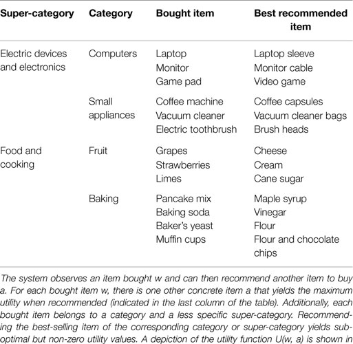
Table 1. Recommender system example.

FIGURE 2

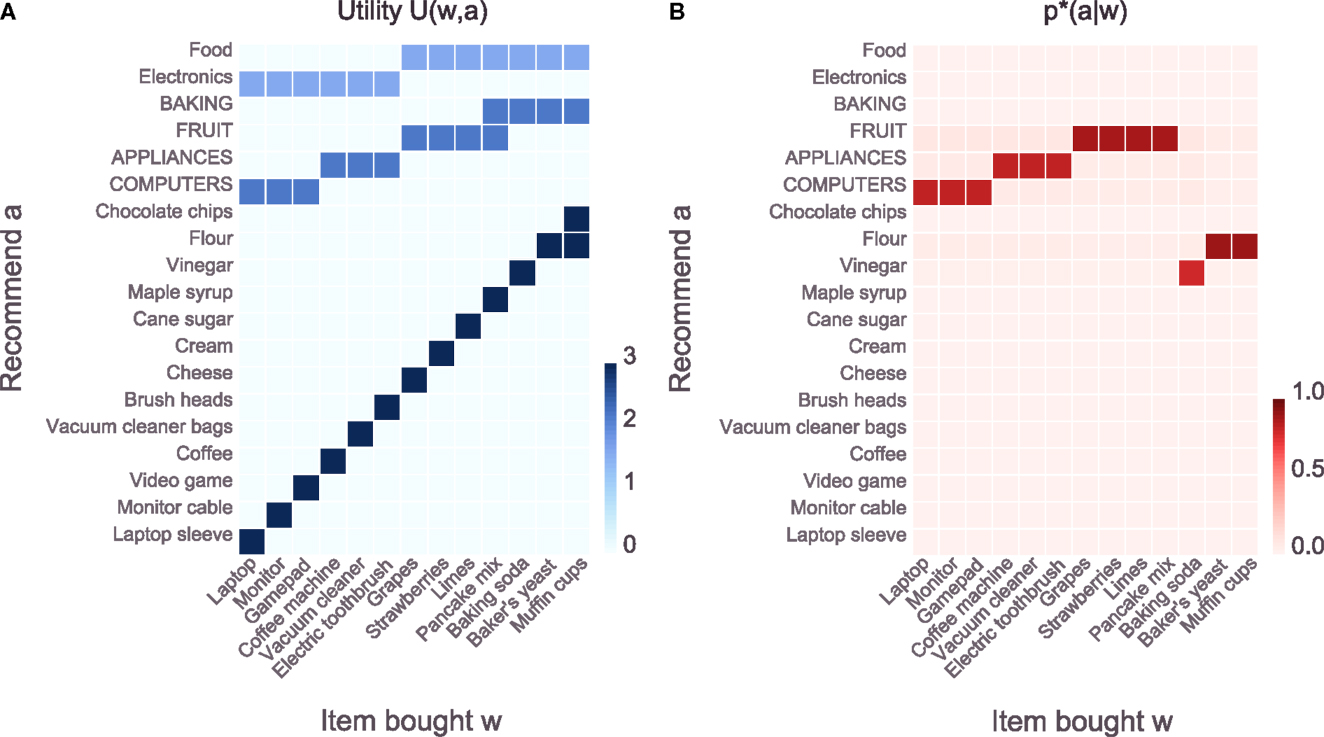
Figure 2. Task setup and solution p*(a|w) for β = 1.3. (A) Utility function U(w, a) for the recommender system task. The recommender system observes an item w bought by a customer and recommends another item a to buy to the customer. For each item bought there is another concrete item that has a high chance of being bought by the customer. Therefore, recommending the correct concrete item leads to the maximum utility of 3. However, each item also belongs to a category (indicated by capital letters) and recommending the best-selling item of the corresponding category leads to a utility of 2.2. Finally, each item also belongs to a super-category (either “food” or “electronics”) and recommending the best-selling item of the corresponding super-category leads to a utility of 1.6. There is one item (muffin cups) where two concrete items can be recommended and both yield maximum utility. Additionally there is one item (pancake mix) where the recommendation of the best-selling item of both categories “fruit” and “baking” yields the same utility. (B) Solution p*(a|w) [equation (9)] for β = 1.3. Due to the low β, the computational resources of the recommender system are quite limited and it cannot recommend the highest scoring items (except in the last three columns). Instead, it saves computational effort by applying the same policy to multiple items.

The utility of each (w, a)-pair is color-coded in blue in Figure 2A. For each possible world-state there is one concrete item that can be recommended that will (deterministically) yield the highest possible utility of 3 utils. Further, each bought item belongs to a category and recommending the best-selling item of the corresponding category leads to a utility of 2.2 utils. Finally, recommending the best-selling item of the corresponding super-category yields a utility of 1.6 utils. For each world-state there is one specific action that leads to the highest possible utility but zero utility for all other world-states. At the same time there exist more abstract actions that are sub-optimal but still “good” for a set of world-states. See the legend of Figure 2 for more details on the example.

Figure 2B shows the result p*(a|w) obtained through Blahut-Arimoto iterations [equations (9) and (10)] for β = 1.3. For each world-state (on the x-axis) the probability over all actions (y-axis) corresponds to one column in the plot and is color-coded in red. For this particular value of β the agent cannot afford to pick the specific actions for most of the world-states (except for the last three world-states) in order to stay within the limit on the maximum allowed rate. Rather, the agent recommends the best-selling items of the corresponding category which allows for a lower rate by having identical policies (i.e., columns in the plot) for sets of world-states. The optimal policies thus lead to abstractions, where several different world-states elicit identical responses of the agent. Importantly, the abstractions are not induced because some stimuli are more similar than others under some utility-free measure and they are also not the result of a post hoc aggregation or clustering scheme. Rather, the abstractions are shaped by the utility function and appear as a consequence of bounded rational decision-making in the given task.

Figure 3A shows the expected utility E _{p( w, a)}[U(w, a)] and the rate-distortion objective J_RD(p(a|w)) as a function of the inverse temperature β. The plot shows that by increasing β the expected utility increases monotonically, whereas the objective J_RD(p(a|w)) also shows a trend to increase but not monotonically. Interestingly, there are a few sharp transitions at the same points in both curves. The same steep transitions are also found in Figure 3B, which shows the mutual information and its decomposition into the entropic terms I(W, A) = H(A) − H(A|W) as a function of β. The line corresponding to the entropy over actions H(A) shows flat plateaus in between these phase transitions. Figure 3C illustrates solutions p^⋆(a|w) for β values corresponding to points on each of the plateaus (labels for bought and recommended items have been omitted for visual compactness but are identical to the plot in Figure 2B). Surprisingly, most of the solutions correspond to different levels of abstraction – from fully abstract for β → 0, then going through several levels of abstraction and getting more and more specific up to the case β → ∞where the conditional entropy H(A|W) goes to zero implying that the conditionals p^⋆(a|w) become deterministic and identical to the maximum expected utility solutions. Within a plateau of H(A), the entropy over actions does not change but the conditional entropy H(A|W) tends to decrease with increasing β. This means that qualitatively the behavior along a plateau does not change in the sense that across all world-states the same subset of actions is used. However, the stochasticity within this subset of actions decreases with increasing β (until at some point a phase-transition occurs). Changing the temperature leads to a natural emergence of different levels of abstraction – levels that emerge from the agent-environment interaction structure described by the utility function. Each level of abstraction corresponds to one plateau in H(A).

FIGURE 3

Figure 3. Sweep overβ values. (A) Evolution of expected utility and value of the objective J_RD(p(a|w)) [equation (7)]. The expected utility is monotonically increasing, the objective also increases with increasing β but not monotonically. In both curves, there are some sharp kinks which indicate a change in level of abstraction (see panels below). (B) Evolution of information quantities. The same sharp kinks as in the panel above can also be seen in all three curves. Interestingly, H(A) has mostly flat plateaus in between these kinks which means that the behavior of the agent does not change qualitatively along the plateau. At the same time, H(A|W) goes down, indicating that behavior becomes less and less stochastic until a phase transition occurs where H(A) changes. (C) Solutions p*(a|w) [equation (9)] that illustrate the agents behavior on each of the plateaus of H(A). It can be seen that on each plateau (and with each kink), the level of abstraction changes.

In general, abstractions are formed by reducing the information content of an entity until it only contains relevant information. For a discrete random variable w ∈ $\mathcal{W}$, this translates into forming a partitioning over the space $\mathcal{W}$ where “similar” elements are grouped into the same subset of $\mathcal{W}$ and become indistinguishable within the subset. In physics, changing the granularity of a partitioning to a coarser level is known as coarse-graining which reduces the resolution of the space $\mathcal{W}$ in a non-uniform manner. Here, the partitioning emerges in p^⋆(a|w) as a soft-partitioning (see Still and Crutchfield, 2007), where “similar” world-states w get mapped to an action a (or a subset of actions) and essentially become indistinguishable. Readers are encouraged to interactively explore the example in the Supplementary Jupyter Notebook “2-RateDistortionForDecisionMaking.”

In analogy to rate-distortion theory where the rate-distortion function serves as an information-theoretic characterization of a system, one can define the rate-utility function

$U\left(R\right)=\underset{p\left(a|w\right):I\left(W;A\right)\le R}{\text{max}}{\mathbf{\text{E}}}_{p\left(w,a\right)}\left[U\left(w,a\right)\right].$ (11)

where the expected utility is a function of the information processing rate I(W; A). If the decision-maker is conceptualized as a communication channel between world-states and actions, the rate I(W; A) defines the minimally required capacity of that channel. The rate-utility function thus specifies the minimum required capacity for computing actions given a certain expected utility target, or analogously the maximally achievable expected utility given a certain information processing capacity. The rate-utility curve is obtained by varying the inverse temperature β (corresponding to different values of R) and plotting the expected utility as a function of the rate. The resulting plot is shown in Figure 4, where the solid line denotes the rate-utility curve and the shaded region corresponds to systems that are theoretically infeasible and cannot be achieved regardless of the implementation. Systems in the white region are sub-optimal, meaning that they could either achieve the same performance with a lower rate or given their limits on computational capacity they could theoretically achieve higher performance. This curve is interesting for both designing systems as well as characterizing the degree of sub-optimality of given systems.

FIGURE 4

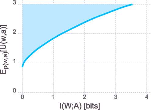
Figure 4. Rate-utility curve. Analogously to the rate-distortion curve in rate-distortion theory, the rate-utility curve shows the minimally required information processing rate to achieve a certain level of expected utility or dually, the maximally achievable expected utility, given a certain rate. Systems that optimally trade-off expected utility against cost of computation lie exactly on the curve. Systems in the shaded region are theoretically impossible and cannot be realized. Systems that lie in the white region of the figure are sub-optimal in the sense that they could achieve a higher expected utility given their computational resources or they could achieve the same expected utility with lower resources.

3. Serial Information-Processing Hierarchies

In this section, we apply the rate-distortion principle for decision-making to a serial perception-action system. We design two stages: a perceptual stage p(x|w) that maps world-states w to observations x and an action stage p(a|x) that maps observations x to actions a. Note that the world-state w does not necessarily have to be considered as a latent variable but could in general also be an observation from a previous processing stage. The action stage implements a bounded rational decision-maker (similar to the one presented in the previous section) that optimally trades off expected utility against cost of computation [see equation (7)]. Classically, the perceptual stage might be designed to represent w as faithfully as possible, given the computational limitations of the perceptual stage. Here, we show that trading off expected utility against the cost of information processing on both the perceptual and the action stage leads to bounded-optimal perception that does not necessarily represent w as faithfully as possible but rather extracts the most relevant information about w such that the action stage can work most efficiently. As a result, bounded-optimal perception will be tightly coupled to the action stage and will be shaped by the utility function as well as the computational capacity of the action channel.

3.1 Optimal Perception is Shaped by Action

To model a perceptual channel we extend the model from Section 2.2 as follows: The agent is no longer capable of fully observing the state of the world W but using its sensors it is capable to form a percept X as p(x|w) which then allows for adaptation of behavior according to p(a|x). The three random variables for world-state, percept, and action form a serial chain of channels, one channel from world-states to percepts expressed by p(x|w) and another channel from percepts to actions expressed by p(a|x) which implies the following conditional independence

$p\left(w,x,a\right)=p\left(w\right)p\left(x|w\right)p\left(a|x\right),$

that is also expressed by the graphical model W → X → A. We assume that p(w) is given and the utility function depends on the world-state and the action U(w, a). Note that mathematically, the results are identical for U(w, x, a), but in this paper we consider the utility independent of the internal percept x.

Classically, inference and decision-making are separated – for instance, by first performing Bayesian inference over the state of the world w using the observation x and then choosing an action a according to the maximum expected utility principle. The MEU action-selection principle can be replaced by a bounded rational model for decision-making that takes into account the computational cost of transforming a (optimal) prior behavior p₀(a) to a posterior behavior p(a|x) as shown in Section 2.

$\begin{array}{l}\text{Bayesian inference}:p\left(w|x\right)=\frac{p\left(w\right)p\left(x|w\right)}{{\sum }_{w}p\left(w\right)p\left(x|w\right)}\end{array}$ (12)

$\begin{array}{l}\text{Bounded rational decision}:p^{\ast }\left(a|x\right)=\frac{1}{Z\left(x\right)}p\left(a\right)e^{{\mathrm{\beta }}_{2}U\left(x,a\right)}\end{array}$ (13)

where U(x, a) = Σ_wp(w|x)U(w, a) is the expectation of the utility under the Bayesian posterior over w given x. Note that the bounded rational decision-maker in equation (13) is identical to the rate-distortion decision-maker introduced in Section 2 that minimizes the trade-off given by equation (7) by implementing equation (9). It includes the MEU solution as a special case for β₂ → ∞. Here, the inverse temperature is denoted by β₂ (instead of β as in the previous section) for notational reasons that ensure consistency with later results of this section.

In equation (12), the choice of the likelihood model p(x|w) remains unspecified and the question is where does it come from? In general, it is chosen by the designer of a system and the choice is often driven by bandwidth or memory constraints. In purely descriptive scenarios, the likelihood model is determined by the sensory setup of a given system and p(x|w) is obtained by fitting it to data of the real system. In the following, we present a particular choice of p(x|w) that is fundamentally grounded on the principle that any transformation of behavior or beliefs is costly (which is identical to the assumption of limited-rate information processing channels) and this cost should be traded off against gains in expected utility. Remarkably, equations (12) and (13) drop out naturally from the principle.

Given the graphical model: W → X → A, we consider an information processing channel between W and X and another one between X and A and introduce different rate-limits on these channels, i.e., the information processing price on the perceptual level ${\frac{1}{\mathrm{\beta }}}_1$ can be different from the price of information processing on the action level ${\frac{1}{\mathrm{\beta }}}_2$. Formally, we set up the following variational problem:

$\begin{array}{l}\underset{p\left(x|w\right),p\left(a|x\right)}{\arg \max }{\mathbf{\text{E}}}_{p\left(w,x,a\right)}\left[U\left(w,a\right)\right]-{\frac{1}{\mathrm{\beta }}}_{1}I\left(W;X\right)-{\frac{1}{\mathrm{\beta }}}_{2}I\left(X;A\right)=\underset{p\left(x|w\right),p\left(a|x\right)}{\arg \max }{J}_{\text{ser}}\left(p\left(x|w\right),p\left(a|x\right)\right).\end{array}$ (14)

Similar to the rate-distortion case, the solution is given by the following set of four self-consistent equations:

$\begin{array}{ll}\hfill p^{\ast }\left(x|w\right)& =\frac{1}{Z\left(w\right)}p\left(x\right)\mathit{exp}\left({\mathrm{\beta }}_1\mathrm{\Delta }{F}_{\text{ser}\left(w,x\right)}\right)\end{array}$ (15)

$\begin{array}{ll}\hfill p\left(x\right)& ={\displaystyle \sum _{w}p\left(w\right)p^{\ast }\left(x|w\right)}\end{array}$ (16)

$\begin{array}{ll}\hfill p^{\ast }\left(a|x\right)& =\frac{1}{Z\left(x\right)}p\left(a\right)\mathit{exp}\left({\mathrm{\beta }}_2{\displaystyle \sum _{w}p\left(w|x\right)U\left(w,a\right)}\right)\end{array}$ (17)

$\begin{array}{ll}\hfill p\left(a\right)& ={\displaystyle \sum _{w,x}p\left(w\right)p^{\ast }\left(x|w\right)p^{\ast }\left(a|x\right)},\end{array}$ (18)

where Z(w) and Z(x) denote the corresponding normalization constants or partition sums. The conditional probability p(w|x) is given by Bayes’ rule $p\left(w|x\right)=\frac{p\left(w\right)p^{\ast }\left(x|w\right)}{p\left(x\right)}$ and ΔF_ser(w, x) is the free energy difference of the action stage:

$\mathrm{\Delta }{F}_{\text{ser}\left(w,x\right)}:={\mathbf{\text{E}}}_{p^{\ast }\left(a|x\right)}\left[U\left(w,a\right)\right]-{\frac{1}{\mathrm{\beta }}}_2{D}_{\text{KL}}\left(p^{\ast }\left(a|x\right)\left|\right|p\left(a\right)\right),$ (19)

see also equation (5). More details on the derivation of the solution equations can be found in the Supplementary Methods Section 2.

The bounded-optimal perceptual model is given by equation (15). It follows the typical structure of a bounded rational solution consisting of a prior times the exponential of the utility multiplied by the inverse temperature. Compare equation (9) to see that the downstream free-energy trade-off ΔF_{ser( w, x)} now plays the role of the utility function for the perceptual model. The distribution p*(x|w) thus optimizes the downstream free-energy difference in a bounded rational fashion, that is taking into account the computational resources of the perceptual channel. Therefore, the optimal percept becomes tightly coupled to the agent-environment interaction structure as described by the utility function or in other words: the optimal percept is shaped by the embodiment of the agent and, importantly, is not simply a maximally faithful representation of W through X given the limited rate of the perceptual channel. A second interesting observation is that the action stage given by equation (17) turns out to be a bounded rational decision-maker using the Bayesian posterior p(w|x) for inferring the true world-state w given the observation x. This is identical to equation (13) (using the optimal prior p(a) = Σ_{w, x} p(w)p*(x|w)p*(a|x)), even though the latter was explicitly modeled by first performing Bayesian inference over the world-state w given the percept x [equation (12)] and then performing bounded rational decision-making [equation (13)], whereas the same principle drops out naturally in equation (17) as a result of optimizing equation (14).

3.2 Illustrative Example

In this section, we design a hand-crafted perceptual model p_λ(x|w) with precision-parameter λ, that drives a subsequent bounded rational decision-maker that maps an observation x to a distribution over actions p(a|x) in order to maximize expected utility while not exceeding a constraint on the rate of the action channel. The latter is implemented by following equation (13) and setting β₂ according to the limit on the rate I(X; A). We compare the bounded rational actor with hand-crafted perception against a bounded-optimal actor that maximizes equation (14) by implementing the four corresponding self-consistent equations (15)–(18). Importantly, the perceptual model p*(x|w) of the bounded-optimal actor maximizes the downstream free-energy trade-off of the action stage ΔF_{ser( w, x)} which leads to a tight coupling between perception and action that is not present in the hand-crafted model of perception. The action stage is identical in both models and given by equation (17).

We designed the following example where the actor is an animal in a predator-prey scenario. The actor has sensors to detect the size of other animals it encounters. In this simplified scenario, animals can only belong to one of three size-groups and their size correlates with their hearing-abilities:

• Small animals (insects): either 2, 3, or 4 size-units cannot hear very well.

• Medium-sized animals (rodents): either 6, 7, or 8 size-units can hear quite well.

• Large animals (cats of prey): either 10, 11, or 12 size-units can hear quite well.

The actor has a sensor for detecting the size of an animal, however, depending on the capacity of the perceptual channel this sensor will either be more or less noisy. To survive, the actor can hunt animals from both the small and the medium-sized group for food. On the other hand, it can fall prey to animals of the large group. The actor has three basic actions:

• Ambush: steadily wait for the other animal to get close and then strike.

• Sneak-up: slowly move closer to the animal and then strike.

• Flee: quickly move away from the other animal.

The advantage of the ambush is that it is silent, however, the risk is that the animal might not move toward the position of the ambush – it works equally well on animals from the small and medium-sized group. The sneak-up is not silent but does not rely on the other animal coincidentally getting closer – it works better than the ambush for small-sized animals but the opposite is true for medium-sized animals. If the actor encounters a large animal the only sensible action is to flee in order to avoid falling prey to the large animal. Besides these generic actions, the actor also has a repertoire of more specific hunting patterns – see Figure 5 which shows the full details of the utility function for the predator-prey scenario. The exact numeric values are found in the Supplementary Jupyter Notebook “3-SerialHierarchy.”

FIGURE 5

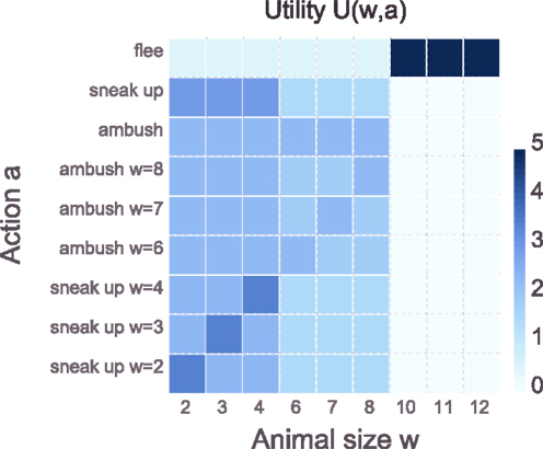
Figure 5. Predator-prey utility function U(w, a). The actor encounters different groups of animals – small, medium-sized, and large – and should hunt small and medium-sized animals for food and flee from large animals. Animals within a group have a similar size w: small animals ∈ {2,3,4} size-units, medium-sized animals ∈ {6,7,8} size-units, and large animals ∈ {10,11,12} size-units. For hunting – denoted by the action a – the actor can either ambush the other animal or alternatively sneak up to the other animal and strike once close enough. In general, sneaking up works well on small animals as they cannot hear very well, whereas medium-sized animals can hear quite well which decreases the chance of a successful sneak-up. The ambush works equally well on both groups of prey. Large animals should never be engaged, but the actor should flee in order to avoid falling prey to them. In addition to the generic hunting patterns that work equally well for all members of a group, for small animals there are specific sneak-up patterns that have an increased chance of success if applied to the correct animal but a decreased chance of success when applied to the wrong animal. For medium-sized animals, there are specific ambush behaviors that have the same chance of success as the generic ambush behavior when applied to the correct animal but a decreased chance of success when applied to the wrong animal. Since the specific ambush behaviors for the medium-sized animals have no advantage over the generic ambush behavior but require more information processing, any bounded rational actor should never choose the specific ambush behaviors. This somewhat artificial construction is meant to illustrate that bounded rational actors do not add unnecessary complexity to their behavior. See main text for more details on the example.

The hand-crafted model of perception is specified by p_λ(x|w), where the observed size x corresponds to the actual size of the animal w corrupted by noise. The precision-parameter λ governs the noise-level and thus the quality of the perceptual channel which can be measured with I(W; X). In particular, the observation o is a discretized noisy version of w with precision λ:

$x|w,\mathrm{\lambda }\sim \text{round}\left({\mathcal{N}}_{\text{trunc}}\left(w,1∕\mathrm{\lambda }\right)\right),$ (20)

where the set of world-states is given by all possible animal sizes w ∈ $\mathcal{W}$ = {2,3,4,6,7,8,10,11,12} and the set of possible observations is given by x ∈ $\mathcal{X}$ = {1,2,3,…,11,12,13}. To avoid a boundary-bias due to the limited interval $\mathcal{X}$we reject and re-sample all values of x that would fall outside of $\mathcal{X}$. For λ → ∞, the perceptual channel is very precise, and there is no uncertainty about the true value of w after observing x. However, such a channel incurs a large computational effort as the mutual information I(W; X) is maximal in this case. If the perceptual channel has a smaller capacity than required to uniquely map each w to an x, the rate must be reduced by lowering the precision λ. Medium precision will mostly lead to within-group confusion whereas low precision will also lead to across-group confusion and corresponds to perceptual channels with a very low rate I(W; X).

The results in Figure 6 show solutions when having large computational resources on both the perception and action channel. As the figure clearly shows, the hand-crafted model p_λ(x|w) looks quite different from the bounded-optimal solution p*(x|w), even though the rate on the perceptual channel is identical in both cases (given by the mutual information I(W; X) ≈ 2 bits). The difference is that the bounded-optimal percept spends the two bits mainly on discriminating between specific animals of the small group and on discriminating between medium-sized and large animals. It does not discriminate between specific sizes within the latter two groups. This makes sense, as there is no gain in utility by applying any specific actions to specific animals in the medium- or large-sized group. Figure 6 also shows the overall-behavior from the point of view of an external observer p(a|w), which is computed as follows

$\begin{array}{l}{p}_{\mathrm{\lambda }}\left(a|w\right)={\displaystyle \sum _x{p}_{\mathrm{\lambda }}\left(x|w\right)p_{\mathrm{\lambda }}\left(a|x\right)}\text{and}{p}^{\ast }\left(a|w\right)={\displaystyle \sum _x{p}^{\ast }\left(x|w\right)p^{\ast }\left(a|x\right)}\end{array}$ (21)

FIGURE 6

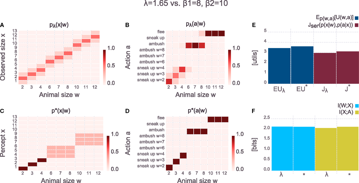
Figure 6. Comparing hand-crafted perception against bounded-optimal perception (parameters are given above the panels). Both the perceptual and the action channel have large computational resources (λ or β₁ for the perceptual channel, respectively, and β₂ for the action channel). (A) Hand-crafted perceptual model p_λ(x|w) [equation (20)] – the observed animal size is a noisy version of the actual size of the animal, but the noise-level is quite low (due to large λ). (B) Overall-behavior of the system p_λ(a|w) [equation (21)] with the hand-crafted perception. For small animals, the specific sneak-up patterns are used, but the noisiness of the perception does not allow to deterministically pick the correct pattern. (C) Bounded-optimal perceptual model p*(x|w) [equation (15)] – the bounded-optimal model does not distinguish between the individual medium- or large-sized animals as all of them are treated with the respective generic action. Instead, the computational resources are spent on precisely discriminating between the different small animals. Note that this bounded-optimal perceptual model spends exactly the same computation as the hand-crafted model [see (F), blue bars]. (D) Overall-behavior p*(a|w) [equation (21)] of the bounded-optimal system. Compared to the hand-crafted system, the bounded-optimal perception allows to precisely discriminate between the different small animals which is also reflected in the overall-behavior. The bounded-optimal system thus achieves a higher expected utility (E). (E) Comparison of expected utility (dark blue, first two columns) and value of the objective [equation (14), dark red, last two columns] for the hand-crafted system (denoted by λ) and the bounded-optimal system (denoted by *). Since both systems spend roughly the same amount of computation [see (F)], but the bounded-optimal model achieves a higher expected utility, the overall objective is in favor of the bounded-optimal system. (F) Comparison of information processing effort in the hand-crafted system (denoted by λ) and the bounded-optimal system (denoted by *). Both systems spend (roughly) the same amount of computation, however, the bounded-optimal system spends it in a more clever way – compare (A,C). The distributions p_λ(a|x) and p*(a|w) are not shown in the figure but can easily be inspected in the Supplementary Jupyter Notebook “3-SerialHierarchy.”

The overall-behavior in the bounded-optimal case is more deterministic, leading to a higher expected utility in the bounded-optimal case. The distributions p_λ(a|x) and p^⋆(a|w) are not shown in the figure but can easily be inspected in the Supplementary Jupyter Notebook “3-SerialHierarchy.” If the price of information processing on the perceptual channel in the hand-crafted model is the same as in the bounded-optimal model (given by β₁), then the overall objective J_ser(p(x|w), p(a|x)) is larger for the bounded-optimal case compared to the hand-crafted case, implying that the bounded optimal actor achieves a better trade-off between expected utility and computational cost. The crucial insight of this example is that the optimal percept depends on the utility function, where in this particular case it does for instance make no sense to waste computational resources on discriminating between the specific animals of the large group because the optimal response (flee with certainty) is identical to all of them. In the Supplementary Jupyter Notebook“3-SerialHierarchy” the utility function can easily be switched while keeping all other parameters identical in order to observe how the bounded-optimal percept changes accordingly. Note that the bounded-optimal behavior p^⋆(a|w) shown in Figure 6D yields the highest possible expected utility in this task setup – there is no behavior that would lead to a higher expected utility (though there are other solutions that lead to the same expected utility).

The bounded-optimal percept depends not only on the utility function but also on the behavioral richness of the actor which is governed by the rate on the action channel I(X; A). In Figure 7 we show the results of the same setup as in Figure 6 with the only change being the significantly increased price for information processing in the action stage (as specified by β₂ = 1 bit per util whereas it used to be β₂ = 10 bits per util in the previous figure). The hand-crafted perceptual model is unaffected by this change of the action stage, but the bounded-optimal model of perception has changed compared to the previous figure and now reflects the limited behavioral richness. As shown in p^⋆(a|w) in Figure 7, the actor is no longer capable of applying different actions to animals of the small group and animals of the medium-sized group. Accordingly, the bounded-optimal percept does not waste computational resources for discriminating between small and medium-sized animals since the downstream policy is identical for both groups of animals. In terms of expected utility, both the hand-crafted model as well as the bounded-optimal decision-maker score equally at ≈3 utils. However, the bounded-optimal model does so by using lower computational resources and thus scoring better on the overall trade-off J_ser(p(x|w), p(a|x)).

FIGURE 7

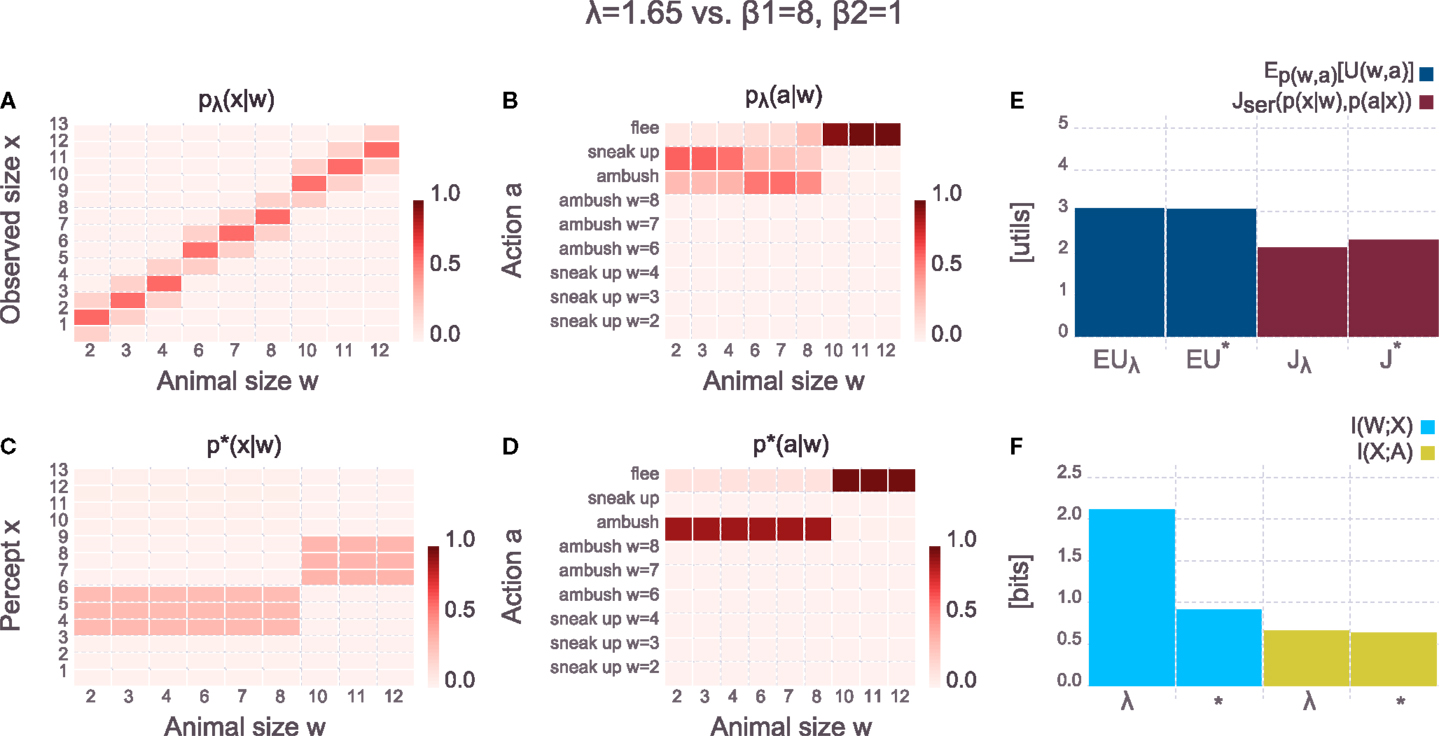
Figure 7. Comparing hand-crafted perception against bounded-optimal perception (parameters are given above the panels). Compared to Figure 6, the action channel of both the hand-crafted and the bounded-optimal system now has low computational resources (through the low β₂ for the action channel). (A) Hand-crafted perceptual model p_λ(x|w) [equation (20)] – the hand-crafted perception is unaffected by the increased limit in computational resources on the action channel. (B) Overall-behavior of the system p_λ(a|w) [equation (21)] with the hand-crafted perception. Even though perception was unaffected by the increased limit on the action channel, the overall-behavior is severely affected. (C) Bounded-optimal perceptual model p*(x|w) [equation (15)] – due to the low information processing rate on the action channel [see (F), yellow bars], the bounded-optimal perception adjusts accordingly and only discriminates between predator and prey animals. (D) Overall-behavior p*(a|w) [equation (21)] of the bounded-optimal system. Compared to the hand-crafted system, the bounded-optimal system distinguishes sharply between predator and prey animals. Note, however, that both systems achieve an identical expected utility [(E), dark blue bars]. (E) Comparison of expected utility (dark blue, first two columns) and value of the objective [equation (14), dark red, last two columns] for the hand-crafted system (denoted by λ) and the bounded-optimal system (denoted by *). Both systems achieve the same expected utility, but the bounded-optimal system does so with requiring less computation on the perceptual channel [see (F), blue bars]. (F) Comparison of information processing effort in the hand-crafted system (denoted by λ) and the bounded-optimal system (denoted by *). Due to the low computational resources on the action channel, the corresponding information processing rate (yellow bars) is quite low. The bounded-optimal perception adjusts accordingly and requires a much lower rate compared to the hand-crafted model of perception that does not adjust. The distributions p_λ(a|x) and p*(a|x) are not shown in the figure but can easily be inspected in the Supplementary Jupyter Notebook “3-SerialHierarchy.”

In Figure 8 we again use large resources on the action channel β₂ = 10 (as in the first example in Figure 6), but now the resources on the perceptual channel are limited by setting β₁ = 1 (compared to β₁ = 8 in the first case). Accordingly, the precision of the hand-crafted perceptual model is tuned to λ = 0.4 (compared to λ = 1.65 in the first case) such that it has the same rate I(W; X) as the bounded-optimal model. By comparing the two panels for p_λ(x|w) and p^⋆(x|w), it can clearly be seen that the bounded-optimal perceptual model now spends its scarce resources to reliably discriminate between large animals and all other animals. The overall behavioral policies p(a|w) reflect the limited perceptual capacity in both cases, however, the bounded-optimal case scores a higher expected utility of ≈3 utils compared to the hand-crafted case. The overall objective J_ser(p(x|w), p(a|x)) is also higher for the bounded-optimal model, indicating that this model should be preferred because it finds a better trade-off between expected utility and information processing cost.

FIGURE 8

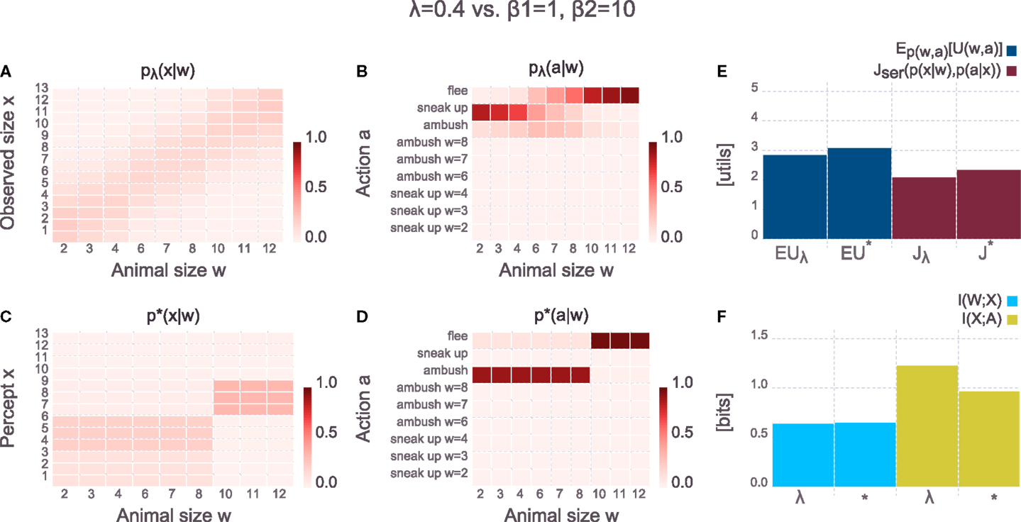
Figure 8. Comparing hand-crafted perception against bounded-optimal perception (parameters are given above the panels). Compared to Figure 6, the perceptual channel of both the hand-crafted and the bounded-optimal system now has low computational resources (through the low λ and β₁ respectively). (A) Hand-crafted perceptual model p_λ(x|w) [equation (20)] – due to the low precision λ, the noise for the hand-crafted perception has increased dramatically. (B) Overall-behavior of the system p_λ(a|w) [equation (21)] with the hand-crafted perception. Even though the action-part of the system still has large computational resources the overall-behavior is severely affected due to the bad perceptual channel. (C) Bounded-optimal perceptual model p*(x|w) [equation (15)] – due to the low computational resources on the perceptual channel (β₁) the system can only distinguish between predator and prey animal (which is the most important information). Note how the percept in the bounded-optimal case no longer corresponds to some observed animal size but rather to a more abstract concept such as predator or prey animal. The parameters were chosen such that both the hand-crafted and the bounded-optimal system spend the same amount of information processing on the perceptual channel [see (F), blue bars]. (D) Overall-behavior p*(a|w) [equation (21)] of the bounded-optimal system. Compared to the hand-crafted system, the bounded-optimal system distinguishes sharply between predator and prey animals. This is only possible because the bounded-optimal perception spends its scarce resource to exactly perform this distinction. (E) Comparison of expected utility (dark blue, first two columns) and value of the objective [equation (14), dark red, last two columns] for the hand-crafted system (denoted by λ) and the bounded-optimal system (denoted by *). The bounded-optimal system achieves a higher expected utility even though the amount of information processing is not larger compared to the hand-crafted model [see (F)]. Rather, the bounded-optimal model spends its scarce resources more optimally. (F) Comparison of information processing effort in the hand-crafted system (denoted by λ) and the bounded-optimal system (denoted by *). Note that both perceptual channels (blue bars) require the same information processing rate, but the bounded-optimal perceptual model processes the more important information (predator versus prey) which allows the subsequent action channel to perform better [see (E), dark blue bars). The distributions p_λ(a|x) and p*(a|x) are not shown in the figure but can easily be inspected in the Supplementary Jupyter Notebook “3-SerialHierarchy.”

Note that in all three examples the optimal percept p^⋆(x|w) often leads to a uniform mapping of an exclusive subset of world-states w to the same set of percepts x. Importantly, these percepts do not directly correspond to an observed animal size as in the case of the hand-crafted model of perception. Rather, the optimal percepts often encode more abstract concepts such as medium- or large-sized animal (as in Figure 6) or predator and prey animal (as in Figures 7 and 8). In a sense, abstractions similar to the ones shown in the recommender system example in the previous section (Figure 3) emerge in the predator-prey example as well but now they also manifest themselves in the form of abstract percepts. Crucially, the abstract percepts allow for more efficient information processing further downstream in the decision-making part of the system. The formation of these abstract percepts is driven by the embodiment of the agent and reflects certain aspects of the utility function of the agent. For instance, unlike the actor in Figure 6, the actors in Figures 7 and 8 would not “understand” the concept of medium-sized animals as it is of no use to them: with their very limited resources it is most important for them to have the two perceptual concepts of predator and prey. Note that the cardinality of X in the bounded-optimal model of perception is fixed in all examples in order to allow for easy comparison against the hand-crafted model, but it could be reduced further without any consequences (up to a certain point) – this can be explored in the Supplementary Jupyter Notebook “3-SerialHierarchy.”

The solutions shown in this section were obtained by iterating the self-consistent equations until numerical convergence. Since there is no convergence-proof, it cannot be fully ruled out that the solutions are sub-optimal with respect to the objective. However, the point of the simulation results shown here is to allow for easier interpretation of the theoretical results and highlight certain aspects of the theoretical findings. We discuss this issue in Section 5.2.

4. Parallel Information- Processing Hierarchies

Rational decision-making requires searching through a set of alternatives a and picking the option with the highest expected utility. Bounded rational decision-making replaces the “hard maximum” operation with a soft selection mechanism where the first action that satisfies a certain level of expected utility is picked. A parallel hierarchical architecture allows for a prior partitioning of the search space which reduces the effective size of the search space and thus speeds up the search process. For instance, consider a medical system that consists of general practitioners and specialist doctors. The general doctor can restrict the search space for a particular ailment of a patient by determining which specialist the patient should see. The specialist doctor in turn can determine the exact disease. This leads to a two-level decision-making hierarchy consisting of a high-level partitioning that allows for making a subsequent low-level decision with reduced (search) effort. In statistics, the partitioning that is induced by the high-level decision is often referred to as a model and is commonly expressed as a probability distribution over the search space p(a|m) (where m indicates the model) which also allows for a soft-partitioning. The advantage of hierarchical architectures is that the computation that leads to the high-level reduction of the search space can be stored in the model (or in a set of parameters in case of a parametric model). This computation can later be re-used by using the correct model (or set of parameters) in order to perform the low-level computation more efficiently. Interestingly, it should be most economic to put the most re-usable, and thus more abstract, information into the models p(a|m) which leads to a hierarchy of abstractions. However, in order to make sure that the correct model is used, another deliberation process p(m|w) is required (where w indicates the observed stimulus or data). Another problem is how to chose the partitioning to be most effective. In this section, we address both problems from a bounded rational point of view. We show that the bounded optimal solution p*(a|m) trades off the computational cost for choosing a model m against the reduction in computational cost for the low-level decision.

To keep the notation consistent across all sections of the paper we denote the model m in the rest of the paper with the variable x. This is in contrast to Section 3, where x played the role of a percept. The advantage of this notation is that it allows to easily see similarities and differences of the information terms and solution equations of the different cases. In particular, in Section 5 we present a unifying case that includes the serial and parallel case as special cases – by keeping the notation consistent this can easily be seen.

4.1 Optimal Partitioning of the Search Space

Constructing a two-level decision-making hierarchy requires the following three components: high-level models p(a|x), a model selection mechanism p(x|w) and a low-level decision maker p(a|w, x) (w denotes the observed world-state, x indicates a particular model and a is an action). The first two distributions are free to be chosen by the designer of the system, for p(a|w, x) a maximum expected utility decision-maker is the optimal choice if computational costs are neglected. Here, we take computational cost into account and replace the MEU decision-maker with a bounded rational decision-maker that includes MEU as a special case (β₃ → ∞) – the bounded rational decision-maker optimizes equation (7) by implementing equation (9). In the following we show how all parts of the hierarchical architecture:

$\begin{array}{l}1.\text{Selection of model (or expert):}p\left(x|w\right)\end{array}$ (22)

$\begin{array}{l}2.\text{Prior knowledge of model (or expert):}p\left(a|x\right)\end{array}$ (23)

$\begin{array}{l}3.\text{Bounded rational decision of model (or expert):}{p}^{\ast }\left(a|w,x\right)=\frac{1}{Z\left(w,x\right)}p\left(a|x\right)e^{{\mathrm{\beta }}_{3}U\left(w,a\right)}\end{array}$ (24)

emerge from optimally trading off computational cost against gains in utility. Importantly, p(a|x) plays the role of a prior distribution for the bounded rational decision-maker and reflects the high-level partitioning of the search space.

The optimization principle that leads to the bounded-optimal hierarchy trades off expected utility against the computational cost of model selection I(W; X) and the cost of the low-level decision using the model as a prior I(W; A|X):

$\begin{array}{l}\hfill \underset{p\left(x|w\right),p\left(a|w,x\right)}{\arg \max }{\mathbf{\text{E}}}_{p\left(w,x,a\right)}\left[U\left(w,a\right)\right]-{\frac{1}{\mathrm{\beta }}}_{1}I\left(W;X\right)-{\frac{1}{\mathrm{\beta }}}_{3}I\left(W;A|X\right)=\underset{p\left(x|w\right),p\left(a|w,x\right)}{\arg \max }{J}_{\text{par}}\left(p\left(x|w\right),p\left(a|w,x\right)\right).\end{array}$ (25)

The set of self-consistent solutions is given by

$\begin{array}{ll}\hfill p^{\ast }\left(x|w\right)& =\frac{1}{Z\left(w\right)}p\left(x\right)\mathit{exp}\left({\mathrm{\beta }}_1\mathrm{\Delta }{F}_{\text{par}\left(w,x\right)}\right)\end{array}$ (26)

$\begin{array}{ll}\hfill p\left(x\right)& ={\displaystyle \sum _{w}p\left(w\right)p^{\ast }\left(x|w\right)}\end{array}$ (27)

$\begin{array}{ll}\hfill p^{\ast }\left(a|w,x\right)& =\frac{1}{Z\left(w,x\right)}{p}^{\ast }\left(a|x\right)\mathit{exp}\left({\mathrm{\beta }}_{3}U\left(w,a\right)\right)\end{array}$ (28)

$\begin{array}{ll}\hfill p^{\ast }\left(a|x\right)& ={\displaystyle \sum _{w}p\left(w|x\right)p^{\ast }\left(a|w,x\right)},\end{array}$ (29)

where Z(w) and Z(w, x) denote the corresponding normalization constants or partition sums. p(w|x) is given by Bayes’ rule $p\left(w|x\right)=\frac{p\left(w\right)p^{\ast }\left(x|w\right)}{p\left(x\right)}$ and ΔF_{par( w, x)} is the free energy difference of the low-level stage:

$\mathrm{\Delta }{F}_{\text{par}}\left(w,x\right):={\mathbf{\text{E}}}_{p^{\ast }\left(a|w,x\right)}\left[U\left(w,a\right)\right]-{\frac{1}{\mathrm{\beta }}}_3{D}_{\text{KL}}\left(p^{\ast }\left(a|w,x\right)\left|\right|p^{\ast }\left(a|x\right)\right),$ (30)

see equation (5). More details on the derivation of the solution equations can be found in the Supplementary Methods Section 3. By comparing the solution equations (26)–(29) with equations (22)–(24) the hierarchical structure of the bounded-optimal solution can be seen clearly. The bounded-optimal model selector in equation (26) maximizes the downstream free-energy trade-off ΔF_{par( w, x)} in a bounded rational fashion and is similar to the optimal perceptual model of the serial case [equation (15)]. This means that the optimal model selection mechanism is shaped by the utility function as well as the computational process on the low-level stage of the hierarchy (governed by β₃) but also by the computational cost of model selection (governed by β₁). The optimal low-level decision-maker given by equation (28) turns out to be exactly a bounded rational decision-maker with p(a|x) as a prior – identical to the low-level decision-maker that was motivated in equation (24). Importantly, the bounded-optimal solution provides a principled way of designing the models p(a|x) [see equation (29)]. According to the equation, the optimal model p^⋆(a|x) is given by a Bayesian mixture over optimal solutions p^⋆(a|w, x) where w is known. The Bayesian mixture turns out to be the optimal compressor of actions for unknown w under the belief p(w|x).

4.2 Illustrative Example

To illustrate the formation of bounded-optimal models, we designed the following example: in a simplified environment, only three diseases can occur – a heart disease or one of two possible lung diseases. Each of the diseases comes in two possible types (e.g., type 1 or type 2 diabetes). Depending on how much information is available on the symptoms of a patient, diseases can be treated according to the specific type (which is most effective) or with respect to the disease category (which is less effective but requires less information). See Figure 9 for a plot of the utility function and a detailed description of the example. The goal is to design a medical analysis hierarchy that initiates the best possible treatment, given its limitations. The hierarchy consists of an automated medical system that can cheaply take standard measurements to partially assess a patient’s disease category. Additionally, the patient is then sent to a specialist who can manually perform more elaborate measurements if necessary to further narrow down the patient’s precise disease type and recommend a treatment. The automated system should be designed in a way that minimizes the additional measurements required by the specialists. More formally, the automated system delivers a first diagnosis x given the patient’s precise disease type w according to p(x|w). The first diagnosis narrows down the possible treatments a according to a model p(a|x). For each x, a specialist can further reduce uncertainty about the correct treatment by performing more measurements p(a|w, x). We compare the optimal design of the automated system and the corresponding optimal treatment recommendations to the specialist p^⋆(a|x) according to equation (29) in two different environments: one, where all disease types occur with equal probability (Figure 9B) versus two, where heart diseases occur with increased chance (Figure 9C). For this example, the number of different high-level diagnoses X is set to |$\mathcal{X}$| = 3 which also means that there can be three different treatment recommendations p(a|x). Since in the example the total budget for performing measurements is quite low (reflected by β₁, β₃ both being quite low), the whole system (automated plus specialists) can in general not gather enough information about the symptoms to treat every disease type with the correct specific treatment. Rather, the low budget has to be spent on gathering the most important information.

FIGURE 9

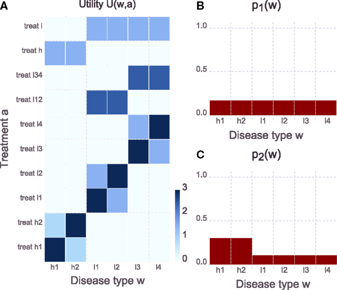
Figure 9. Task setup of the medical system example. (A) Utility function. The disease category heart disease comes in the two types h1 or h2. There are two different categories of lung diseases that come in types l1 or l2 (lung disease A) or types l3 and l4 (lung disease B). The goal of the medical system is to gather information about the disease type and then initiate a treatment. Each of the disease types is best treated with a specific treatment. However, when the specific treatment is applied to the wrong disease type of the same disease category it is less effective. Additionally there are general treatments for the heart- and the two lung diseases that are slightly worse than the specific treatments but can be applied with less knowledge about the disease type. For lung diseases, there is a general treatment that works even if the specific lung disease is not known; however, it is less effective compared to the treatments where the disease but not the precise type is known. (B) Distribution of disease types in environment 1 – all diseases appear with equal probability. (C) Distribution of disease types in environment 2 where the heart diseases have an increased probability and the two corresponding disease types appear with higher chance.

Figure 10 shows bounded-optimal hierarchies for the medical system in both environments. The top row in Figure 10 shows the optimal hierarchy for the environment where all diseases appear with equal probability: the automated system p^⋆(x|w) (see Figure 10A) distinguishes between a heart disease, lung disease A and lung disease B, which means that there is one treatment recommendation for heart diseases and one treatment recommendation for each of the two possible lung diseases respectively (see the three columns of p^⋆(a|x) in Figure 10B). Since the general treatment for the heart disease works less effective than the general treatments for the two lung diseases, the (very limited) budget of the specialists is completely spent on finding the correct specific heart treatment. Both lung diseases are treated with their respective general treatments since the two lung specialists have no budget for additional measurements. Since the automated system already distinguishes between the two lung diseases, it can narrow down the possible treatments to a delta over the correct general treatment, thus requiring no additional measurements by the lung specialists (shown by the two columns in p^⋆(a|x) that have a delta over the treatment).

FIGURE 10

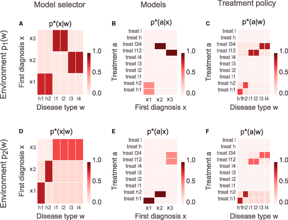
Figure 10. Bounded-optimal hierarchies for two different environments (different p(w)). Top row: all disease types are equally probable, bottom row: heart diseases and thus h1 and h2 are more probable. (A,D) Optimal model (or specialist) selectors [equation (26)]. In the uniform environment it is optimal to have one specialist for each disease category (heart, lung A, and lung B) and have a model selector that maps specific disease types to the corresponding specialist x. In the non-uniform environment it is optimal to have one specialist for each of the two types of the heart disease (h1, h2) and another one for all lung diseases. The corresponding model selector in the bottom row reflects this change in the environment. (B,E) Optimal models [equation (29), each column corresponds to one specialist]. The resources of the specialists are very limited due to a very low β₃, meaning that the average deviation of p*(a|w, x) from p*(a|x) must be small. In the uniform environment it is optimal that the heart specialist spends all the resources for discriminating between the two heart disease types because using the general heart treatment on both types is less effective compared to using one of the lung disease treatments on both corresponding types. In the non-uniform environment this is reversed as the specialists for h1 and h2 do not need any more measurements to determine the correct treatment, however, the remaining budget (of 1 bit) is spent on discriminating between the two categories of lung diseases (but is insufficient for discriminating between the four possible lung disease types). (C,F) Overall-behavior of the hierarchical system p*(a|w) = Σ_xp*(x|w)p*(a|w, x). The distributions p*(a|w, x) [equation (28)] are not shown in the figure but can easily be investigated in the Supplementary Jupyter Notebook “4-ParallelHierarchy.”

The bottom row in Figure 10 shows the optimal hierarchy for the environment where heart diseases appear with higher probability. In this case it is optimal to redesign the automated system to distinguish between the two types of the heart disease h1, h2, and lung diseases in general (see p^⋆(x|w) in Figure 10D of the figure). This means that there are now treatment recommendations p^⋆(a|x) for h1 and h2 that do not require any more measurements by the specialists (shown by the delta over a treatment in the first two columns of p^⋆(a|x) in Figure 10E) and there is another treatment recommendation for lung diseases. The corresponding specialist can use the limited budget to perform additional measurements to distinguish between the two categories of lung disease (but not between the four possible types as this would require more measurements than the budget allows). The example illustrates how the bounded-optimal decision-making hierarchy is shaped by the environment and emerges from optimizing the trade-off between expected utility and overall information processing cost. Readers can interactively explore the example in the Supplementary Jupyter Notebook “4-ParallelHierarchy” – in particular by changing the information processing costs of the specialists β₃ or changing the number of specialists by increasing or decreasing the cardinality of X.

The solutions shown in this section were obtained by iterating the self-consistent equations until numerical convergence. Since there is no convergence-proof, it cannot be fully ruled out that the solutions are sub-optimal with respect to the objective. However, the point of the simulation results shown here is to allow for easier interpretation of the theoretical results and highlight certain aspects of the theoretical findings. We discuss this issue in Section 5.2.

4.3 Comparing Parallel and Serial Information Processing

In order to achieve a certain expected utility, a certain overall rate I(W; A) is needed. In the one-step rate-distortion case (Section 2) the channel from w to a must have a capacity larger or equal to that rate. In the serial case (Section 3) there is a channel from w to x and another channel from x to a. Both serial channels must at least have a capacity of I(W; A) in order to achieve the same overall rate, as the following inequality always holds for the serial case

$I\left(W;A\right)\le \text{min}\left\{I\left(W;X\right),I\left(X;A\right)\right\}.$

In contrast, the parallel architecture allows for computing a certain overall rate I(W; A) using channels with a lower capacity because the contribution in reducing uncertainty about a on each level of the hierarchy splits up as follows:

$\underset{\text{total}\text{reduction}}{\underbrace{I\left(W,X;A\right)}}=\underset{\text{high}-\text{level}}{\underbrace{I\left(X;A\right)}}+\underset{\text{low}-\text{level}}{\underbrace{I\left(W;A|X\right)}},$

which implies I(W, X; A) ≥ I(X; A). In particular, if the low-level step contributes information then I(W; A|X) > 0 and the previous inequality becomes strict. The same argument also holds when considering I(W; A) (see Section 5.1).

In many scenarios the maximum capacity of a single processing element is limited and it is desirable to spread the total processing load on several elements that require a lower capacity. For instance, there could be technical reasons why processing elements with 5 bits of capacity can easily be manufactured but processing elements with a capacity of 10 bits cannot be manufactured or are disproportionally more costly to produce. In the one-step case and the serial case the only way to stay below a certain capacity limit is by tuning β until the required rate is below the capacity – however, in both cases this also decreases the overall rate I(W; A). In the parallel hierarchical case several building blocks with a limited capacity can be used to produce an overall rate I(W; A) larger than the capacity of each processing block.

Splitting of information processing load onto several processing blocks is illustrated in Figure 11, where the one-step and parallel hierarchical solutions to the medical example are compared. In this example, the price of information processing in the one-step case is quite low (β = 10 bits per util) such that the corresponding solution leads to a deterministic mapping of each w to the best a (see Figure 11A). Doing so requires I(W; A) ≈ 2.6 bits (see Figure 11B). Now assume for the sake of this example that processing elements, where information processing cost is reduced (15 bits per util), could be manufactured, but the maximum capacity of these elements is 1.58 bits. In the one-step case these processing elements can only be used if it is acceptable to reduce the rate I(W; A) to 1.58 bits (by tuning β) which would imply a lower expected utility. However, in the parallel hierarchical case the new processing elements can be used (see Figure 11C) which leads to a reduced price of information processing (β₁ = 15, β₃ = 14.999). In conjunction the new processing elements process the same effective information I(W; A) (see Figure 11D) and achieve the same expected utility as the one-step case (see Figure 11B). However, since the price for information processing is lower on the more limited elements, the overall trade-off between expected utility and information processing cost is in favor of the parallel hierarchical architecture. Note that in this example it is important that the cardinality of X is limited (in this case |$\mathcal{X}$| = 3) and β₁ > β₃. We discuss this in the next paragraphs.

FIGURE 11

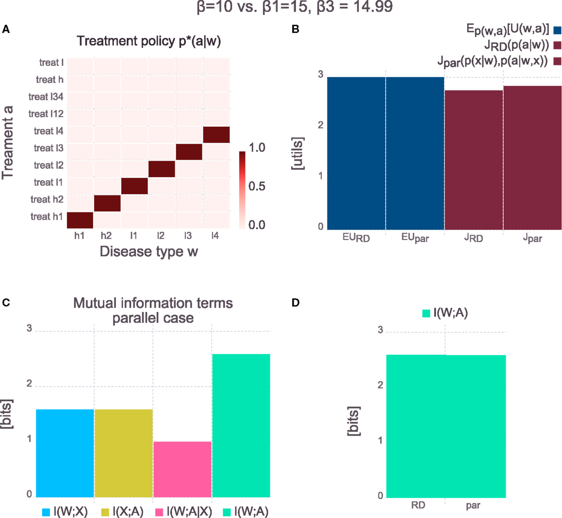
Figure 11. Bounded-optimal parallel hierarchy (denoted by “par”) versus one-step (rate-distortion) case (denoted by “RD”). (A) Overall-behavior p*(a|w) = Σ_xp*(x|w)p*(a|w, x). The overall-behavior is identical for the one-step case and the parallel hierarchical solution. Due to the low price of information processing each w is deterministically mapped to the best a. (B) Comparison of performance of one-step (“RD”) and parallel case (“par”). Both solutions achieve the same expected utility but the hierarchical solution has a better trade-off between expected utility and information processing cost (because the price of information processing is lower in the hierarchical case ${\frac{1}{\mathrm{\beta }}}_1$, ${\frac{1}{\mathrm{\beta }}}_3$ compared to $\frac{1}{\mathrm{\beta }}$ in the one-step case) since in the hierarchical case the cheap but capacity-limited processing elements can be used – see main text). J_RD(p(a|w)) corresponds to equation (7) and J_par(p(x|w), p(a|w, x)) corresponds to equation (25). (C) Mutual information terms of the parallel case I(W; X), I(X; A), I(W; A|X), and I(W; A) (from left to right). The individual processing channels in the hierarchical case are all within the capacity limit of 1.58 bits, but the overall processed information I(W; A) is ≈2.6 bits. (D) Comparison of “effective” information I(W; A) processed in the parallel case (denoted by “par”) and the information processed in the one-step (rate-distortion) case (denoted by “RD”). I(W; A) is identical for the one-step and the hierarchical case, but in the parallel case it was computed in a distributed fashion, where each computational step (or channel) has a rate lower than I(A; W) [see (C)]. The figure can be reproduced with the Supplementary Jupyter Notebook “5-DistributionOfInformationProcessing.”

In the parallel hierarchical case, there are two possible pathways from w to a:

$\begin{array}{ll}\hfill \text{Two-stage serial pathway}& I\left(W;X\right)\to I\left(X;A\right)\\ \hfill \text{Parallel pathway}& I\left(W;A|X\right)\end{array}$

Note that I(X; A) does not appear in the objective [equation (25)]; however, it is crucial for distributing information processing on both levels of the hierarchy (see more analysis of the medical system example in Figure 11). I(X; A) measures the average adaptation effort for going from p(a) to p(a|x). In the parallel hierarchical case it is a measure of how much the different models p(a|x) narrow down the search space compared to the average p(a) = Σ_xp(x)p(a|x). If all models are equal p(a|x) = p(a) ∀x the mutual information I(X; A) is zero. Note, however, that a large I(X; A) is rendered useless by a low I(W; X) and vice versa – if the model selector is very bad, even the best models are not useful and vice versa.

Since there is no cost for having a large rate I(X; A), the overall throughput of the serial pathway is effectively governed by β₁ as it affects the rate I(W; X). Similarly, β₃ governs the rate on the parallel pathway I(W; A|X). As a result, whenever one of the two inverse temperatures β₁ and β₃ is larger than the other, it becomes more economic to shift all the information processing to the cheaper pathway (either serial or parallel) thus rendering the other pathway obsolete. The only scenario where it can be advantageous to use both pathways (and distribute computation) is when the cheaper pathway has insufficient capacity and the more expensive pathway is used to take on additional computational load that cannot be handled by the cheap pathway alone. Effectively, this translates into the constraint that the serial pathway must be cheaper β₁ > β₃ and additionally the serial pathway must be limited in its capacity by limiting the cardinality |$\mathcal{X}$| (see Supplementary Methods Section 5 for a detailed discussion).

Note the important difference between changing the cardinality of X which governs the channel capacity of the serial pathway (that is the maximally possible rates I(W; X), I(X; A)) but has no influence on the price of information processing and changing β₁ which governs the price of processing I(W; X) and hence affects the actual rate on the serial pathway but has no effect on the capacity of the channels of the serial pathway.

$\begin{array}{ll}\hfill I\left(W;X\right)& =H\left(X\right)-H\left(X|W\right)\le \mathbf{\text{H}}\left(\mathbf{\text{X}}\right)\end{array}$ (31)

$\begin{array}{ll}\hfill I\left(X;A\right)& =H\left(A\right)-H\left(A|X\right)=H\left(X\right)-H\left(X|A\right)\le \mathbf{\text{H}}\left(\mathbf{\text{X}}\right)\end{array}$ (32)

$\begin{array}{ll}\hfill I\left(W;A|X\right)& =H\left(A|X\right)-H\left(A|W,X\right)\le H\left(A|X\right)\end{array}$ (33)

H(X) is an upper bound for both I(W; X) but also I(X; A) and the upper bound of H(X) itself is a function of |$\mathcal{X}$|. Note that since there is no cost associated with I(X; A) it is generally desirable to maximize I(X; A) at least such that I(X; A) ≥ I(W; X). To do so H(A|X) must be pushed toward zero [equation (32)] – however, this simultaneously pushes the upper bound for I(W; A|X) toward zero [equation (33)]. In case of a sufficiently limited H(X) (through a low |$\mathcal{X}$|), I(X; A) cannot be fully maximized, therefore leaving a non-zero upper bound for I(W; A|X).

In the example shown in Figure 11 information processing is performed on both the serial pathway (I(W; X) and I(X; A)) but also on the parallel pathway (I(W; A|X)) because the constraints for distribution of information processing are fulfilled: β₁ > β₃ and the capacity (that is the maximum rate I(W; X) and I(X; A)) of the serial pathway is limited by the (low) cardinality |$\mathcal{X}$| = 3. The cardinality of X for the example can easily be changed in the Supplementary Jupyter Notebook “4-ParallelHierarchy” – if it is for instance increased to |$\mathcal{X}$| = 6 while keeping all other parameters the same, the whole information processing load will be entirely on the serial pathway and I(W; A|X) = 0. Alternatively to limiting the cardinality of X, a cost for I(X; A) could be introduced to limit the computational resources for computing p(a|x) from p(a). This is explored in Section 5.

5. Toward More General Architectures

In the serial case in Section 3, information processing cost arises from adapting p(x) to p(x|w) and p(a) to p(a|x), and the average informational effort is measured by I(W; X) and I(X; A). In the parallel hierarchical case in Section 4 the two information processing terms considered are I(W; X) and I(W; A|X), where the latter measures the average informational effort for adapting from p(a|x) to p(a|w, x). In this section, we present a mathematically unifying case that considers all three mutual information terms and includes the serial and the parallel case as special cases. This unifying formulation might also be a starting point for generalizing toward more than three random variables as the corresponding objective function could easily be extended to include more variables.

The general case uses the same factorization of the three variables W, X, A as the parallel case: p(w, x, a) = p(w)p(x|w)p(a|w, x). Given this factorization, the KL-divergence between the joint p(w, x, a) and the product of all three marginals, also known as the total correlation C(W, X, A), leads to:

$\begin{array}{l}\hfill C\left(W,X,A\right)=D_{\text{KL}}\left(p\left(w,x,a\right)\left|\right|p\left(w\right)p\left(x\right)p\left(a\right)\right)=H\left(W\right)+H\left(X\right)+H\left(A\right)-H\left(W,X,A\right)\\ ={\displaystyle \sum _{w,x,a}p\left(w,x,a\right)\log \frac{p\left(w,x,a\right)}{p\left(w\right)p\left(x\right)p\left(a\right)}}\\ ={\displaystyle \sum _{w,x}p\left(w,x\right)\log \frac{p\left(x|w\right)}{p\left(x\right)}}+{\displaystyle \sum _{w,a,x}p\left(w,x,a\right)\log \frac{p\left(a|w,x\right)}{p\left(a\right)}}\end{array}$ (34)

$\begin{array}{ll}\hfill & =I\left(W;X\right)+I\left(W,X;A\right)\end{array}$ (35)

$\begin{array}{l}=I\left(W;X\right)+I\left(X;A\right)+I\left(W;A|X\right).\end{array}$ (36)

The total correlation (Watanabe, 1960), also called multivariate constraint (Garner, 1962) or multiinformation (Studenỳ and Vejnarová, 1998), is the sum of the three information processing terms considered in the serial and parallel case. The general objective is formed by assigning different prices to each of the terms and trading off the resulting information processing cost against the expected utility:

$\begin{array}{l}\underset{p\left(x|w\right),p\left(a|w,x\right)}{\arg \max }{\mathbf{\text{E}}}_{p\left(w,x,a\right)}\left[U\left(w,a\right)\right]-{\frac{1}{\mathrm{\beta }}}_{1}I\left(W;X\right)-{\frac{1}{\mathrm{\beta }}}_{2}I\left(X;A\right)-{\frac{1}{\mathrm{\beta }}}_{3}I\left(W;A|X\right)\\ =\underset{p\left(x|w\right),p\left(a|w,x\right)}{\arg \max }{J}_{\text{gen}}\left(p\left(x|w\right),p\left(a|w,x\right)\right).\end{array}$ (37)

Identical to the parallel hierarchical case, the general case has two information processing pathways that allow for splitting up the total computational load: a serial pathway consisting of the two stages I(W; X) and I(X; A) and a parallel pathway I(W; A|X). If any of the pathways is cheaper than the other one, it is more economical to shift all the computation to the cheaper pathway. However, the capacity of the serial pathway can be limited, for example by reducing the cardinality of X. In such a case the parallel pathway can take on additional computational load, leading to a parallel hierarchical information processing architecture.

The solution to the general objective is given by the following set of five self-consistent equations (the detailed derivation of the solutions is included in the Supplementary Methods Section 1):

$\begin{array}{l}\hfill p^{\ast }\left(x|w\right)=\frac{1}{Z\left(w\right)}p\left(x\right)\exp \left(\right.{\mathrm{\beta }}_1\mathrm{\Delta }{F}_{\text{gen}}\left(w,x\right)-\left(\frac{{\mathrm{\beta }}_1}{{\mathrm{\beta }}_3}-\frac{{\mathrm{\beta }}_1}{{\mathrm{\beta }}_2}\right)D_{\text{KL}}\left(p^{\ast }\left(a|w,x\right)\left|\right|p^{\ast }\left(a|x\right)\right)\left)\right.\end{array}$ (38)

$\begin{array}{ll}\hfill p\left(x\right)& ={\displaystyle \sum _{w}p\left(w\right)p^{\ast }\left(x|w\right)}\end{array}$ (39)

$\begin{array}{ll}\hfill p^{\ast }\left(a|w,x\right)& =\frac{1}{Z\left(w,x\right)}{p}^{\ast }\left(a|x\right)\exp \left({\mathrm{\beta }}_{3}U\left(w,a\right)-\frac{{\mathrm{\beta }}_3}{{\mathrm{\beta }}_2}\log \frac{p^{\ast }\left(a|x\right)}{p\left(a\right)}\right)\end{array}$ (40)

$\begin{array}{ll}\hfill p^{\ast }\left(a|x\right)& ={\displaystyle \sum _{w}p\left(w|x\right)p^{\ast }\left(a|w,x\right)}\end{array}$ (41)

$\begin{array}{ll}\hfill p\left(a\right)& ={\displaystyle \sum _{w,x}p\left(w\right)p^{\ast }\left(x|w\right)p^{\ast }\left(a|w,x\right)},\end{array}$ (42)

where Z(w) and Z(w, x) denote the corresponding normalization constants or partition sums. The conditional distribution p(w|x) is given by Bayes’ rule $p\left(w|x\right)=\frac{p\left(w\right)p^{\ast }\left(x|w\right)}{p\left(x\right)}$ and ΔF_{gen( w, x)} is the free energy difference

$\mathrm{\Delta }{F}_{\text{gen}}\left(w,x\right):={\mathbf{\text{E}}}_{p^{\ast }\left(a|w,x\right)}\left[U\left(w,a\right)\right]-{\frac{1}{\mathrm{\beta }}}_2{D}_{\text{KL}}\left(p^{\ast }\left(a|w,x\right)\left|\right|p\left(a\right)\right).$

For β₃ < β₂ the KL-term in equation (38) has a positive sign, implying that the KL-divergence is a utility instead of a cost which makes sense if computation on I(W; A|X) is cheaper than computation on I(A|X). For β₃ > β₂ the KL-term gets a negative sign, implying that the KL-divergence is a cost, as a result of computation on I(W; A|X) being more expensive than computation on I(A|X).

Equation 38 can also be rewritten as (see Supplementary Methods Section 1.2):

$\begin{array}{l}{p}^{\ast }\left(x|w\right)=\frac{1}{Z\left(w\right)}p\left(x\right)\exp \left(\right.{\mathrm{\beta }}_1\mathrm{\Delta }{F}_{\text{par}}\left(w,x\right)-\frac{{\mathrm{\beta }}_1}{{\mathrm{\beta }}_2}{\displaystyle \sum _a}{p}^{\ast }\left(a|w,x\right)\log \frac{p^{\ast }\left(a|x\right)}{p\left(a\right)}\left)\right.\end{array}$ (43)

where ΔF_{par( w, x)} is the same free energy difference as in the parallel case

$\begin{array}{l}\hfill \mathrm{\Delta }{F}_{\text{par}}\left(w,x\right):={\mathbf{\text{E}}}_{p^{\ast }\left(a|w,x\right)}\left[U\left(w,a\right)\right]-{\frac{1}{\mathrm{\beta }}}_3{D}_{\text{KL}}\left(p^{\ast }\left(a|w,x\right)\left|\right|p^{\ast }\left(a|x\right)\right)\end{array}$ (44)

see equation (30).

Comparing the objective in equation (37) with the objective of the parallel case in equation (25), it can be seen that by setting β₂ → ∞the two objective functions become equal and the implicit assumption that in the parallel case there is no cost for going from p(a) to p(a|x) (as the latter is considered a prior) is made explicit. The solution equations of the general case also collapse to the solutions of the parallel case by letting β₂ → ∞: compare equations (43) and (40) against equations (26) and (28). The general case thus also allows for designing more realistic hierarchical cases where there is a small cost for switching models p^⋆(a|x) that arises, for instance, from loading a certain set of parameters or switching to a particular sampler or reading the model from memory. Similarly, the serial case can be recovered by β₃ → 0. The special cases of the general objective are summarized in Table 2.

TABLE 2

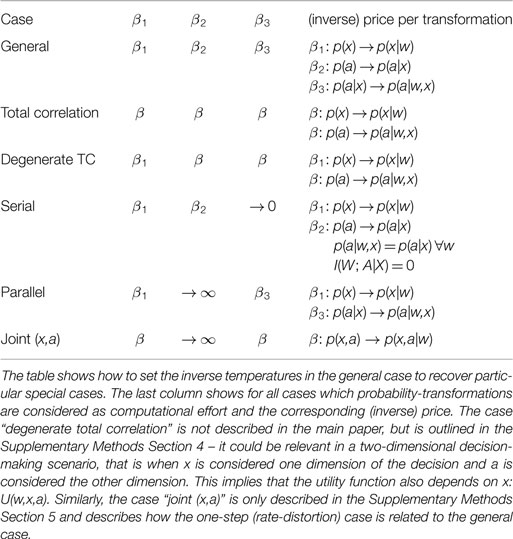
Table 2. Recovery of special cases from the general, unifying case by specific settings of the inverse temperatures.

5.1 Effective Information Throughput I(W; A)

The amount of information processing that effectively contributes toward achieving a high expected utility is measured by I(W; A) which does not directly appear in the objective of the general case (nor the serial and parallel case). However, the effective information throughput of the system is given by

$\begin{array}{ll}\hfill I\left(W;A\right)& =I\left(W;X;A\right)+I\left(W;A|X\right)\end{array}$ (45)

$\begin{array}{l}=I\left(W;X\right)+I\left(X;A\right)-I\left(X;W,A\right)+I\left(W;A|X\right)\end{array}$ (46)

$\begin{array}{l}=C\left(W,X,A\right)-I\left(X;W,A\right)\end{array}$ (47)

where I(W; X; A) denotes the multivariate mutual information (MMI; Yeung, 1991). The first equation above is obtained by re-ordering the definition of the MMI I(K; L; M) = I(K; M) − I(K; M|L). Note that in the serial hierarchical case I(W; A|X) = 0 always holds. The equations above also show how the total correlation C(W, X, A) and the MMI I(W; X; A) are related.

The multivariate mutual information is upper-bounded by I(W; X; A) ≤ min{I(W; X), I(W; A), I(X; A)} (see (Yeung, 1991)). Using the bound in equation (45) leads to and upper bound for the effective information throughput:

$I\left(W;A\right)\le \text{min}\left\{I\left(W;X\right),I\left(X;A\right)\right\}+I\left(W;A|X\right)$ (48)

Equation 48 shows how information processing in the general case can be distributed between a two-stage serial pathway (consisting of I(W; X) and I(X; A)) and a parallel pathway (I(W; A|X)). The general case forms a parallel hierarchy similar to Section 4, but it allows to associate a cost with I(X; A) (which is a measure of how costly it is to switch models). Importantly the discussion on splitting up information processing between both levels of the parallel hierarchy as in Section 4.3 also holds for the general case.

5.2 Iterating the Self-Consistent Equations

For the simulation results shown in this paper the corresponding set of self-consistent equations was iterated until convergence (by checking that the total change in probability distributions between two iteration steps is below a certain threshold – see code underlying the Supplementary Notebooks for details). This is inspired by the Blahut-Arimoto scheme that is proven to converge to the global maximum in the rate-distortion case (Csiszar, 1974; Cover and Thomas, 1991) (Section 2). Unfortunately there is no such proof for iterating the sets of self-consistent equations of the general, serial or parallel case. It is not clear whether the optimization problems are still convex and have a global solution, nor is it clear that iterating the self-consistent equations would converge toward these global solutions. A convexity and convergence analysis is certainly among the most important steps for future investigations of the principles presented here. At this point, we can only report empirical observations and interested readers are encouraged to explore convergence behavior using the Supplementary Jupyter Notebooks (which include plots that show convergence behavior across iterations) but also the underlying code (published in the Supplementary Material).

6. Discussion and Conclusion

The overarching principle behind this paper is the consistent application of the trade-off of gains in expected utility against the computational cost that these gains require. Here, computational cost is defined as the average effort of computational adaptation (measured by the mutual information) multiplied by the price of information processing. This definition is motivated by first principles (Mattsson and Weibull, 2002; Ortega and Braun, 2010; Ortega and Braun, 2011) and is grounded in a thermodynamic framework for decision-making (Ortega and Braun, 2013). Mathematically, the basic principle is identical to the principle behind rate-distortion theory, the information-theoretic framework for lossy compression (Genewein and Braun, 2013; Still, 2014). This connection is no coincidence as bounded rational decision-making can be cast as a lossy compression problem in lossy compression the goal is to transmit the most relevant information (given the limited channel capacity) in order to minimize a distortion-function. In bounded rational decision-making the goal is to process the most relevant information in order maximize a utility function, given the limitations on information processing. In Section 2, we have shown how different levels of behavioral abstraction can be induced by different computational limitations. The authors in (van Dijk and Polani, 2013) use the Relevant Information method, which is a particular application of rate-distortion theory and find a very similar emergence of “natural abstractions” and “ritualized behavior” when studying goal-directed behavior in the MDP case. We have shown how the basic principle can be extended to more complex cases and that analytic solutions can be obtained for these cases. Importantly, the solutions allow for interesting interpretations, highlighting how the same fundamental trade-off can lead to systems that elegantly solve more complex problems. For instance, when designing a perception-action system, the perceptual part of the system can easily be understood as a lossy compressor, but the corresponding distortion-function is not intuitively clear. We have shown in Section 3 how the extended lossy compression principle leads to a well-defined distortion-function for the perceptual part of the system that optimizes the downstream trade-off between expected utility and computational cost. In a similar fashion we have shown in Section 4 how the problem of designing bounded-optimal decision-making hierarchies is fundamentally equal to designing a distributed lossy compressor (that is spread over both levels of the hierarchy).

In the serial hierarchy in Section 3, we compared a perceptual channel that performs Bayesian inference against a bounded-optimal perceptual channel that optimizes the downstream free energy trade-off. We found that the difference between both models of perception was that in one case the likelihood model p(x|w) was unspecified (Bayesian inference) whereas in the other case it was well defined (bounded-optimal solution). Perception is often conceptualized as (Bayesian) inference, however, given our findings there is a subtle but important difference. In our model of a perception-action system, the goal of the perceptual model p(x|w) is to extract the most relevant information from w for choosing an action according to p(a|x), given the computational limitations of the system. In plain inference, the goal is to predict w from x very well and the likelihood model is thus chosen to maximize predictive power. In many cases the two objectives coincide as achieving a large expected utility often requires precise knowledge about w. However, this must not always be the case and in particular for systems where computational limitations play a large role, the (limited) computational resources can often be spent more economically which allows for a higher expected utility at the cost of not being able to predict w from x that well. An interesting machine-learning application of the serial principle could be the design of optimal features for classification.

In Section 4, we showed how parallel bounded-optimal decision-making hierarchies can emerge from solving the trade-off between utility and cost of computation. We found that the condition for parallel hierarchies to being optimal solutions was that the price for model selection is lower than the price for processing information on the low level of the hierarchy (β₁ > β₃). At the same time, the upper level of the hierarchy must be limited in capacity (for instance through the cardinality |$\mathcal{X}$|). Intuitively this makes sense and fits with the general observation that often hardware that allows for cheap information processing is itself quite expensive to build (low signal to noise ratio, etc.). Therefore the amount of hardware that allows for cheap information processing is likely to be quite limited. It remains an open question whether this is a fundamental constraint for hierarchies being optimal solutions or whether there are other arguments in favor of hierarchical architectures. In changing environments, for example, the overall change required to adapt a system is smaller for a hierarchical system, compared to a flat system, because the more abstract levels of the hierarchy might require little or no change at all. It could also be that the upper levels of a hierarchical model based on our principle contain more transferable knowledge that can be applied to novel but similar tasks. Changing the task corresponds to changing the utility-function, which requires a non-equilibrium analysis (Grau-Moya and Braun, 2013) that we leave for future investigation.

In our simulations, we initialize p(x|w) and either p(a|w, x) (parallel hierarchies) or p(a|x) (serial hierarchies) and iterate the equations until (numerical) convergence. We found sometimes that the solutions can be sensitive to the initialization. This hints at the problem being non-convex or the iteration-scheme being prone to get stuck in local optima or plateaus. In particular, we find that in the serial hierarchy with low cost of computation, a sparse, diagonal-like initialization of p(x|w) works much better than a random initialization. For the parallel hierarchies, we found that a random or sparse initialization of p(x|w) combined with a uniform initialization of p(a|w, x) works most reliably. Additionally we found that in the hierarchical case if β₃ is slightly larger than β₁ the iterations converge to sub-optimal solutions where both pathways are used instead of shifting all the computation to the parallel pathway. The toy simulations presented here are illustrative examples only and numerically efficient implementations of the iteration-schemes are beyond the scope of the current paper. These problems might be addressed by other solution schemes like sampling-based or parametric model-based solutions. Nevertheless, these other solution schemes (that potentially do not even require the sets of analytical solutions) can benefit from the interpretations given by the analytic solution equations in this paper.

The ability to form abstractions is thought of as a hallmark of intelligence, both in cognitive tasks and in basic sensorimotor behaviors (Kemp et al., 2007; Braun et al., 2010a,b; Gershman and Niv, 2010; Tenenbaum et al., 2011; Genewein and Braun, 2012). Traditionally, the formation of abstractions is conceptualized as being computationally costly because particular entities have to be grouped together by neglecting irrelevant information. Recently, abstractions that arise from sensory evolution and hierarchical behaviors have been studied from an information-theoretic perspective (Salge and Polani, 2009; Van Dijk et al., 2011). Here, we study abstractions in the process of decision-making, where “similar” situations elicit the same behavior when partially ignoring the current situational context. Extending our principle to hierarchies with more than two levels might provide novel points of view on the formation of hierarchies in biological systems, such as the early visual system (DiCarlo et al., 2012). One fundamental prediction, based on our current work is that the formation of abstractions and concepts should be heavily shaped by the agent-environment structure (the utility function). Following the work of (Simon, 1972) decision-making with limited information-processing resources has been studied extensively in psychology, economics, political science, industrial organization, computer science, and artificial intelligence research. In this paper, we use an information-theoretic model of decision-making under resource constraints (McKelvey and Palfrey, 1995; Kappen, 2005; Wolpert, 2006; Todorov, 2009; Peters et al., 2010; Theodorou et al., 2010; Rubin et al., 2012). In particular, Braun et al. (2011) and Ortega and Braun (2011, 2012, 2013) present a framework in which gain in expected utility is traded off against the adaptation cost of changing from an initial behavior to a posterior behavior. The variational problem that arises due to this trade-off has the same mathematical form as the minimization of a free energy difference functional in thermodynamics. Here, we discuss the close connection between the thermodynamic decision-making framework (Ortega and Braun, 2013) and rate-distortion theory which is an information-theoretic framework for lossy compression. The problem in lossy compression is essentially the problem of separating structure from noise and is thus highly related to finding abstractions (Tishby et al., 1999; Still and Crutchfield, 2007; Still et al., 2010). In the context of decision-making the rate-distortion framework can be applied by conceptualizing the decision-maker as a channel from observations to actions with limited capacity, which is known in economics as the framework of “Rational Inattention” (Sims, 2003).

The rate-distortion principle and all the extended principles presented in this paper measure computational cost with the mutual information which is an abstract measure that quantifies the average KL-divergence. The mutual information measures the actual transformation of probabilities and thus provides a lower bound for any possible implementation. In fact, different implementations could perform the same transformation more or less efficiently which should reflect in the price of information processing but not the amount of information processed. The advantage of using a generic measure is that the principle is universal and can be applied to any system. The downside of this is that it cannot be directly used to analyze specific implementations. In practice it can be hard to determine how difficult or “costly” it is to implement a certain transformation of probability distributions. Rather, the price for information processing is often set implicitly, for instance by certain computation-time constraints or by constraining the number of samples, etc. When applying the principle to a specific implementation it might be required to derive a novel, specific solution scheme for the corresponding optimization problem. In Leibfried and Braun (2015), for instance, the authors apply the rate-distortion principle for decision-making to a spiking neuron model by deriving a gradient-based update rule for tuning the parameters of the model (the weights of the neuron). In their case, the price of information processing β appears directly in the parameter update equations which leads to an interesting regularizer for the (online) parameter update rule.

The fundamental trade-off between large expected utility and low computational cost appears in many domains such as machine learning, AI, economics, computational biology or neuroscience, and many solutions, such as heuristics, sampling-based approaches, and model-based approximation schemes, exist (Gershman et al., 2015; Jordan and Mitchell, 2015; Parkes and Wellman, 2015). One of the exciting prospects of such an approach is that it might provide a common ground for research-questions from artificial intelligence and neuroscience, thus partially unifying the two fields that share common origins but have drifted apart over the last decades (Gershman et al., 2015). The main contribution of this paper is to advance a principled mathematical framework that formalizes the problem objective such that the trade-off between large expected utility and low computational cost and its solutions can be addressed in both a qualitative but also quantitative way. The main finding is that the consistent application of the principle beyond simple one-stage information processing systems leads to non-trivial solutions that address questions like optimal likelihood model design or the design of optimal decision-making hierarchies. Since the mathematics can easily be extended to more variables while the underlying principle remains the same, we believe that the formulation presented in this paper is a good candidate for a general underlying objective that is also applicable to biological organisms and evolutionary processes. We find the principle an interesting starting point for solving timely problems in machine learning, robotics, and AI but also for providing an interesting novel angle for research in computational neuroscience and biology. The principle also provides a promising basis for the design and analysis of guided self-organizing systems as most of the inner structure of systems following our principle is emergent (and thus self-organized) but ultimately aimed at solving particular tasks (through the utility function).

Authors Contribution

TG and DB conceived the project, TG and JG performed simulations, TG and FL did analysis and derivations, and TG, FL, JG, and DB wrote the paper.

Conflict of Interest Statement

The authors declare that the research was conducted in the absence of any commercial or financial relationships that could be construed as a potential conflict of interest.

Funding

This study was supported by the DFG, Emmy Noether grant BR4164/1-1.

Supplementary Material

The Supplementary Material for this article can be found online at https://www.frontiersin.org/article/10.3389/frobt.2015.00027

A Supplementary Methods provides detailed steps to derive the solution to the general case (Section 5) and how to rewrite the solution equations of the general case. Additionally it outlines how to derive the solutions for the serial and the parallel case. It also provides the set of self-consistent equations for the “degenerate total correlation” and “total correlation” case that drop out mathematically from the general case but are not used in this paper (see Table 2). The Supplementary Methods provides details to the discussion on the different information processing pathways of the parallel case (Section 4.3). Finally, it contains the proof for the inequality based on equation (6).

The simulations underlying the results presented in this paper are published as supplementary material using Jupyter (http://jupyter.org/) notebooks. The notebooks are considered part of the results of this paper and readers are encouraged to use the notebooks to interactively explore the examples and concepts presented here. The underlying code is written in Julia (Bezanson et al., 2014) and uses the Gadfly package (http://gadflyjl.org/) for visualization. At the time of writing, the notebooks can be run with a local installation of Jupyter and Julia or without any installation in a web-browser through the JuliaBox project (https://www.juliabox.org/). The notebooks and code at the time of publication are provided in a supplementary.zip file but also under (Genewein, 2015). The notebooks and the code behind the notebooks as well as information on different methods to run the notebooks will be kept up-to-date in the accompanying GitHub repository: https://github.com/tgenewein/BoundedRationalityAbstraction AndHierarchicalDecisionMaking. If compatibility issues with future Julia versions are encountered, please refer to the GitHub repository and feel free to submit an issue. A readme-file on how to run the notebooks (with or without installation) is also provided in the supplementary data as well as in the GitHub repository.

The following notebooks are provided:

• “1-FreeEnergyForBoundedRationalDecisionMaking”: Illustrates the results of Section 1 and reproduces Figure 1.

• “2-RateDistortionForDecisionMaking”: Illustrates the results of Section 4 (the recommender system example) and reproduces Figures 2–4. The notebook can be used as a general template for setting up any of the examples presented in the paper and solving it using Blahut-Arimoto.

• “S1-SampleBasedBlahutArimoto”: A simple proof-of-concept implementation of sample-based Blahut-Arimoto iterations. Due to space-constraints, this part has been omitted from the paper, but interested readers can find a short theoretical part on the sampling approach in the notebook. Additionally, the notebook shows an implementation of the sampling scheme and applies it to a toy example.

• “3-SerialHierarchy”: Illustrates the comparison between hand-crafted perception and bounded-optimal perception in the serial case (Section 3) using the predator-prey example. The notebook reproduces Figures 5–8. The notebook allows to easily modify the parameters (e.g., inverse temperatures) of the example or to switch to a different utility function. It can also be used to see how the parallel or general case solution for the predator-prey example would look like.

• “4-ParallelHierarchy”: Illustrates the emergence of bounded-optimal hierarchies in two different environments of the medical system example as presented in Section 4 and reproduces Figures 9 and 10. The notebook can be used to easily explore the different information processing pathways in the parallel case but also to compare any two cases against each other (because it compares two general case solutions and they can be tuned to all of the special cases).

• “5-DistributionOfInformationProcessing”: Compares the parallel hierarchical solution to the medical example to the one-step (rate-distortion) case as shown in Figure 11. Since it implements the parallel case through the general case, it also allows to compare any other case to the one-step solution.

References

Arimoto, S. (1972). An algorithm for computing the capacity of arbitrary discrete memoryless channels. IEEE Trans. Inf. Theory 18, 14–20. doi: 10.1109/TIT.1972.1054753

CrossRef Full Text | Google Scholar

Ashby, W. R. (1956). An Introduction to Cybcernetics. London: Chapman & Hall.

Google Scholar

Bezanson, J., Edelman, A., Karpinski, S., and Shah, V. B. (2014). Julia: a fresh approach to numerical computin. arXiv preprint arXiv:1411.1607.

Google Scholar

Bishop, C. M. (2006). “Sampling methods,” in Pattern Recognition and Machine Learning, Number 4 in Information Science and Statistics, Chap. 11 (New York: Springer).

Google Scholar

Blahut, R. (1972). Computation of channel capacity and rate-distortion functions. IEEE Trans. Inf. Theory 18, 460–473. doi:10.1109/TIT.1972.1054855

CrossRef Full Text | Google Scholar

Braun, D. A., Mehring, C., and Wolpert, D. M. (2010a). Structure learning in action. Behav. Brain Res. 206, 157–165. doi:10.1016/j.bbr.2009.08.031

CrossRef Full Text | Google Scholar

Braun, D. A., Waldert, S., Aertsen, A., Wolpert, D. M., and Mehring, C. (2010b). Structure learning in a sensorimotor association task. PLoS ONE 5:e8973. doi:10.1371/journal.pone.0008973

CrossRef Full Text | Google Scholar

Braun, D. A., and Ortega, P. A. (2014). Information-theoretic bounded rationality and epsilon-optimality. Entropy 16, 4662–4676. doi:10.3390/e16084662

CrossRef Full Text | Google Scholar

Braun, D. A., Ortega, P. A., Theodorou, E., and Schaal, S. (2011). “Path integral control and bounded rationality,” in IEEE Symposium on Adaptive Dynamic Programming and Reinforcement Learning (Piscataway: IEEE), 202–209.

Google Scholar

Burns, E., Ruml, W., and Do, M. B. (2013). Heuristic search when time matters. J. Artif. Intell. Res. 47, 697–740. doi:10.1613/jair.4047

CrossRef Full Text | Google Scholar

Camerer, C. (2003). Behavioral Game Theory: Experiments in Strategic Interaction. Princeton, NY: Princeton University Press.

Google Scholar

Cover, T. M., and Thomas, J. A. (1991). Elements of Information Theory. Hoboken: John Wiley & Sons.

Google Scholar

Csiszar, I. (1974). On the computation of rate-distortion functions. IEEE Trans. Inf. Theory 20, 122–124. doi:10.1109/TIT.1974.1055146

CrossRef Full Text | Google Scholar

Csiszár, I., and Tusnády, G. (1984). Information geometry and alternating minimization procedures. Stat. Decis. 1, 205–237.

Google Scholar

Daniel, C., Neumann, G., and Peters, J. (2012). “Hierarchical relative entropy policy search,” in International Conference on Artificial Intelligence and Statistics. La Palma.

Google Scholar

Daniel, C., Neumann, G., and Peters, J. (2013). “Autonomous reinforcement learning with hierarchical REPS,” in International Joint Conference on Neural Networks. Dallas.

Google Scholar

DiCarlo, J. J., Zoccolan, D., and Rust, N. C. (2012). How does the brain solve visual object recognition? Neuron 73, 415–434. doi:10.1016/j.neuron.2012.01.010

PubMed Abstract | CrossRef Full Text | Google Scholar

Fox, C. W., and Roberts, S. J. (2012). A tutorial on variational Bayesian inference. Artif. Intell. Rev. 38, 85–95. doi:10.1007/s10462-011-9236-8

CrossRef Full Text | Google Scholar

Friston, K. (2010). The free-energy principle: a unified brain theory? Nat. Rev. Neurosci. 11, 127–138. doi:10.1038/nrn2787

PubMed Abstract | CrossRef Full Text | Google Scholar

Garner, W. R. (1962). Uncertainty and Structure as Psychological Concepts. New York: Wiley.

Google Scholar

Genewein, T. (2015). Bounded rationality, abstraction and hierarchical decision-making: an information-theoretic optimality principle: supplementary code (v1.1.0). Zenodo. doi:10.5281/zenodo.32410

CrossRef Full Text | Google Scholar

Genewein, T., and Braun, D. A. (2012). A sensorimotor paradigm for Bayesian model selection. Front. Hum. Neurosci. 6:291. doi:10.3389/fnhum.2012.00291

PubMed Abstract | CrossRef Full Text | Google Scholar

Genewein, T., and Braun, D. A. (2013). Abstraction in decision-makers with limited information processing capabilities. arXiv preprint arXiv:1312.4353.

Google Scholar

Gershman, S. J., Horvitz, E. J., and Tenenbaum, J. B. (2015). Computational rationality: a converging paradigm for intelligence in brains, minds, and machines. Science 349, 273–278. doi:10.1126/science.aac6076

PubMed Abstract | CrossRef Full Text | Google Scholar

Gershman, S. J., and Niv, Y. (2010). Learning latent structure: carving nature at its joints. Curr. Opin. Neurobiol. 20, 251–256. doi:10.1016/j.conb.2010.02.008

PubMed Abstract | CrossRef Full Text | Google Scholar

Gigerenzer, G., and Brighton, H. (2009). Homo heuristicus: why biased minds make better inferences. Top. Cogn. Sci. 1, 107–143. doi:10.1111/j.1756-8765.2008.01006.x

PubMed Abstract | CrossRef Full Text | Google Scholar

Gigerenzer, G., and Todd, P. M. (1999). Simple Heuristics That Make Us Smart. Oxford: Oxford University Press.

Google Scholar

Grau-Moya, J., and Braun, D. A. (2013). Bounded rational decision-making in changing environments. arXiv preprint arXiv:1312.6726.

Google Scholar

Horvitz, E. (1988). “Reasoning under varying and uncertain resource constraints,” in AAAI, Vol. 88 (Palo Alto: AAAI), 111–116.

Google Scholar

Horvitz, E., and Zilberstein, S. (2001). Computational tradeoffs under bounded resources. Artif. Intell. 126, 1–4. doi:10.1016/S0004-3702(01)00051-0

CrossRef Full Text | Google Scholar

Horvitz, E. J., Cooper, G. F., and Heckerman, D. E. (1989). “Reflection and action under scarce resources: theoretical principles and empirical study,” in Proceedings of the 11th International Joint Conference on Artificial Intelligence, Vol. 2 (Detroit: Morgan Kaufmann Publishers, Inc.), 1121–1127.

Google Scholar

Howes, A., Lewis, R. L., and Vera, A. (2009). Rational adaptation under task and processing constraints: implications for testing theories of cognition and action. Psychol. Rev. 116, 717–751. doi:10.1037/a0017187

PubMed Abstract | CrossRef Full Text | Google Scholar

Janssen, C. P., Brumby, D. P., Dowell, J., Chater, N., and Howes, A. (2011). Identifying optimum performance trade-offs using a cognitively bounded rational analysis model of discretionary task interleaving. Top. Cogn. Sci. 3, 123–139. doi:10.1111/j.1756-8765.2010.01125.x

PubMed Abstract | CrossRef Full Text | Google Scholar

Jones, B. D. (2003). Bounded rationality and political science: lessons from public administration and public policy. J. Public Adm. Res. Theory 13, 395–412. doi:10.1093/jopart/mug028

CrossRef Full Text | Google Scholar

Jordan, M., and Mitchell, T. (2015). Machine learning: trends, perspectives, and prospects. Science 349, 255–260. doi:10.1126/science.aaa8415

PubMed Abstract | CrossRef Full Text | Google Scholar

Kahneman, D. (2003). Maps of bounded rationality: psychology for behavioral economics. Am. Econ. Rev. 93, 1449–1475. doi:10.1257/000282803322655392

CrossRef Full Text | Google Scholar

Kappen, H. J. (2005). Linear theory for control of nonlinear stochastic systems. Phys. Rev. Lett. 95, 200–201. doi:10.1103/PhysRevLett.95.200201

CrossRef Full Text | Google Scholar

Kappen, H. J., Gómez, V., and Opper, M. (2012). Optimal control as a graphical model inference problem. Mach. Learn. 87, 159–182. doi:10.1007/s10994-012-5278-7

CrossRef Full Text | Google Scholar

Kemp, C., Perfors, A., and Tenenbaum, J. B. (2007). Learning overhypotheses with hierarchical Bayesian models. Dev. Sci. 10, 307–321. doi:10.1111/j.1467-7687.2007.00585.x

PubMed Abstract | CrossRef Full Text | Google Scholar

Leibfried, F., and Braun, D. A. (2015). A reward-maximizing spiking neuron as a bounded rational decision maker. Neural Comput. 27, 1686–1720. doi:10.1162/NECO_a_00758

PubMed Abstract | CrossRef Full Text | Google Scholar

Levy, R. P., Reali, F., and Griffiths, T. L. (2009). “Modeling the effects of memory on human online sentence processing with particle filters,” in Advances in Neural Information Processing Systems (Vancouver: NIPS), 937–944.

Google Scholar

Lewis, R. L., Howes, A., and Singh, S. (2014). Computational rationality: linking mechanism and behavior through bounded utility maximization. Top. Cogn. Sci. 6, 279–311. doi:10.1111/tops.12086

PubMed Abstract | CrossRef Full Text | Google Scholar

Lieder, F., Griffiths, T., and Goodman, N. (2012). “Burn-in, bias, and the rationality of anchoring,” in Advances in Neural Information Processing Systems (Lake Tahoe: NIPS), 2690–2798.

Google Scholar

Lipman, B. (1995). Information processing and bounded rationality: a survey. Can. J. Econ. 28, 42–67. doi:10.2307/136022

CrossRef Full Text | Google Scholar

Mattsson, L. G., and Weibull, J. W. (2002). Probabilistic choice and procedurally bounded rationality. Games Econ. Behav. 41, 61–78. doi:10.1016/S0899-8256(02)00014-3

CrossRef Full Text | Google Scholar

McKelvey, R. D., and Palfrey, T. R. (1995). Quantal response equilibria for normal-form games. Games Econ. Behav. 10, 6–38. doi:10.1006/game.1995.1023

CrossRef Full Text | Google Scholar

Neal, R. M. (2003). Slice sampling. Ann. Stat. 31, 705–767. doi:10.1214/aos/1056562461

CrossRef Full Text | Google Scholar

Neymotin, S. A., Chadderdon, G. L., Kerr, C. C., Francis, J. T., and Lytton, W. W. (2013). Reinforcement learning of two-joint virtual arm reaching in a computer model of sensorimotor cortex. Neural Comput. 25, 3263–3293. doi:10.1162/NECO_a_00521

PubMed Abstract | CrossRef Full Text | Google Scholar

Ortega, P., and Braun, D. (2010). “A conversion between utility and information,” in Third Conference on Artificial General Intelligence (AGI 2010) (Lugano: Atlantis Press), 115–120.

Google Scholar

Ortega, P. A., and Braun, D. A. (2014). Generalized Thompson sampling for sequential decision-making and causal inference. Complex Adapt. Syst. Model. 2, 269–274. doi:10.1186/2194-3206-2-2

CrossRef Full Text | Google Scholar

Ortega, P. A., Braun, D. A., and Tishby, N. (2014). “Monte Carlo methods for exact & efficient solution of the generalized optimality equations,” in Proceedings of IEEE International Conference on Robotics and Automation. Hong Kong.

Google Scholar

Ortega, P. A., and Braun, D. A. (2011). “Information, utility and bounded rationality,” in Proceedings of the 4th International Conference on Artificial General Intelligence (Mountain View: Springer-Verlag), 269–274.

Google Scholar

Ortega, P. A., and Braun, D. A. (2012). “Free energy and the generalized optimality equations for sequential decision making,” in Journal of Machine Learning Research: Workshop and Conference Proceedings (Edinburgh: JMLR W&C Proceedings), 1–10.

Google Scholar

Ortega, P. A., and Braun, D. A. (2013). Thermodynamics as a theory of decision-making with information-processing costs. Proc. R. Soc. A Math. Phys. Eng. Sci. 469, 2153.

Google Scholar

Palmer, S. E., Marre, O., Berry, M. J., and Bialek, W. (2015). Predictive information in a sensory population. Proc. Natl. Acad. Sci. U.S.A. 112(22), 6908–6913. doi:10.1073/pnas.1506855112

PubMed Abstract | CrossRef Full Text | Google Scholar

Parkes, D. C., and Wellman, M. P. (2015). Economic reasoning and artificial intelligence. Science 349, 267–272. doi:10.1126/science.aaa8403

PubMed Abstract | CrossRef Full Text | Google Scholar

Peters, J., Mülling, K., and Altun, Y. (2010). “Relative entropy policy search,” in AAAI. Atlanta.

Google Scholar

Ramsey, F. P. (1931). “Truth and probability,” in The Foundations of Mathematics and Other Logical Essays, ed. R. B. Braithwaite (New York, NY: Harcourt, Brace and Co), 156–198.

Google Scholar

Rawlik, K., Toussaint, M., and Vijayakumar, S. (2012). “On stochastic optimal control and reinforcement learning by approximate inference,” in Proceedings Robotics: Science and Systems. Sydney.

Google Scholar

Rubin, J., Shamir, O., and Tishby, N. (2012). “Trading value and information in mdps,” in Decision Making with Imperfect Decision Makers (Springer), 57–74.

Google Scholar

Rubinstein, A. (1998). Modeling Bounded Rationality. Cambridge: MIT Press.

Google Scholar

Russell, S. (1995). “Rationality and intelligence,” in Proceedings of the Fourteenth International Joint Conference on Artificial Intelligence, ed. C. Mellish (San Francisco, CA: Morgan Kaufmann), 950–957.

Google Scholar

Russell, S. J., and Norvig, P. (2002). Artificial Intelligence: A Modern Approach. Upper Saddle River: Prentice Hall.

Google Scholar

Russell, S. J., and Subramanian, D. (1995). Provably bounded-optimal agents. J. Artif. Intell. Res. 2, 575–609.

Google Scholar

Salge, C., and Polani, D. (2009). Information-driven organization of visual receptive fields. Adv. Complex Syst. 12, 311–326. doi:10.1142/S0219525909002234

CrossRef Full Text | Google Scholar

Sanborn, A. N., Griffiths, T. L., and Navarro, D. J. (2010). Rational approximations to rational models: alternative algorithms for category learning. Psychol. Rev. 117, 1144. doi:10.1037/a0020511

PubMed Abstract | CrossRef Full Text | Google Scholar

Savage, L. J. (1954). The Foundations of Statistics. New York: Wiley.

Google Scholar

Shannon, C. E. (1948). A mathematical theory of communication. Bell Syst. Tech. J. 27, 379–423, 623–656. doi:10.1002/j.1538-7305.1948.tb00917.x

CrossRef Full Text | Google Scholar

Simon, H. A. (1955). A behavioral model of rational choice. Q. J. Econ. 69, 99–118. doi:10.2307/1884852

CrossRef Full Text | Google Scholar

Simon, H. A. (1972). Theories of bounded rationality. Decis. Organ. 1, 161–176.

Google Scholar

Sims, C. A. (2003). Implications of rational inattention. J. Monet. Econ. 50, 665–690. doi:10.1016/S0304-3932(03)00029-1

CrossRef Full Text | Google Scholar

Sims, C. A. (2005). “Rational inattention: a research agenda,” in Deutsche Bundesbank Spring Conference, Number 4. Berlin.

Google Scholar

Sims, C. A. (2006). Rational inattention: beyond the linear-quadratic case. Am. Econ. Rev. 96, 158–163. doi:10.1257/000282806777212431

CrossRef Full Text | Google Scholar

Sims, C. A. (2010). “Rational inattention and monetary economics,” in Handbook of Monetary Economics, Vol. 3, Chap. 4 (Elsevier), 155–181.

Google Scholar

Spiegler, R. (2011). Bounded Rationality and Industrial Organization. Oxford: Oxford University Press.

Google Scholar

Still, S. (2009). Information-theoretic approach to interactive learning. Europhys. Lett. 85, 28005. doi:10.1209/0295-5075/85/28005

CrossRef Full Text | Google Scholar

Still, S. (2014). “Lossy is lazy,” in Workshop on Information Theoretic Methods in Science and Engineering (Helsinki: University of Helsinki), 17–21.

Google Scholar

Still, S., and Crutchfield, J. P. (2007). Structure or noise? arXiv preprint arXiv:0708.0654.

Google Scholar

Still, S., Crutchfield, J. P., and Ellison, C. J. (2010). Optimal causal inference: estimating stored information and approximating causal architecture. Chaos 20, 037111. doi:10.1063/1.3489885

PubMed Abstract | CrossRef Full Text | Google Scholar

Studenỳ, M., and Vejnarová, J. (1998). “The multiinformation function as a tool for measuring stochastic dependence,” in Learning in Graphical Models (New York: Springer), 261–297.

Google Scholar

Tenenbaum, J. B., Kemp, C., Griffiths, T. L., and Goodman, N. D. (2011). How to grow a mind: statistics, structure, and abstraction. Science 331, 1279–1285. doi:10.1126/science.1192788

PubMed Abstract | CrossRef Full Text | Google Scholar

Theodorou, E., Buchli, J., and Schaal, S. (2010). A generalized path integral control approach to reinforcement learning. J. Mach. Learn. Res. 11, 3137–3181.

Google Scholar

Tishby, N., Pereira, F. C., and Bialek, W. (1999). “The information bottleneck method,” in The 37th Annual Allerton Conference on Communication, Control, and Computing.

Google Scholar

Tishby, N., and Polani, D. (2011). “Information theory of decisions and actions,” in Perception-Action Cycle, Chap. 19 (New York: Springer), 601–636.

Google Scholar

Tkačik, G., and Bialek, W. (2014). Information processing in living systems. arXiv preprint arXiv:1412.8752.

Google Scholar

Todorov, E. (2007). “Linearly-solvable Markov decision problems,” in Advances in Neural Information Processing Systems (Vancouver: NIPS), 1369–1376.

Google Scholar

Todorov, E. (2009). Efficient computation of optimal actions. Proc. Natl. Acad. Sci. U.S.A. 106, 11478–11483. doi:10.1073/pnas.0710743106

PubMed Abstract | CrossRef Full Text | Google Scholar

Tversky, A., and Kahneman, D. (1974). Judgment under uncertainty: heuristics and biases. Science 185, 1124–1131. doi:10.1126/science.185.4157.1124

PubMed Abstract | CrossRef Full Text | Google Scholar

van Dijk, S. G., and Polani, D. (2013). Informational constraints-driven organization in goal-directed behavior. Adv. Complex Syst. 16:1350016. doi:10.1142/S0219525913500161

CrossRef Full Text | Google Scholar

Van Dijk, S. G., Polani, D., and Nehaniv, C. L. (2011). “Hierarchical behaviours: getting the most bang for your bit,” in Advances in Artificial Life: Darwin Meets von Neumann, eds. R. Goebel, J. Siekmann, and W. Wahlster (New York: Springer), 342–349.

Google Scholar

Von Neumann, J., and Morgenstern, O. (1944). Theory of Games and Economic Behavior. Princeton: Princeton University Press.

Google Scholar

Vul, E., Alvarez, G., Tenenbaum, J. B., and Black, M. J. (2009). “Explaining human multiple object tracking as resource-constrained approximate inference in a dynamic probabilistic model,” in Advances in Neural Information Processing Systems (New York: Wiley), 1955–1963.

Google Scholar

Vul, E., Goodman, N., Griffiths, T. L., and Tenenbaum, J. B. (2014). One and done? Optimal decisions from very few samples. Cogn. Sci. 38, 599–637. doi:10.1111/cogs.12101

PubMed Abstract | CrossRef Full Text | Google Scholar

Watanabe, S. (1960). Information theoretical analysis of multivariate correlation. IBM J. Res. Dev. 4, 66–82. doi:10.1147/rd.41.0066

CrossRef Full Text | Google Scholar

Wiener, N. (1961). Cybernetics or Control and Communication in the Animal and the Machine, Vol. 25. Cambridge: MIT press.

Google Scholar

Wolpert, D. H. (2006). “Information theory-the bridge connecting bounded rational game theory and statistical physics,” in Complex Engineered Systems, eds D. Braha, A. A. Minai, and Y. Bar-Yam (New York: Springer), 262–290.

Google Scholar

Yeung, R. W. (1991). A new outlook on Shannon’s information measures. IEEE Trans. Inf. Theory 37, 466–474. doi:10.1109/18.79902

CrossRef Full Text | Google Scholar

Yeung, R. W. (2008). Information Theory and Network Coding. New York: Springer.

Google Scholar