Design of Introspective Circuits for Analysis of Cell-Level Dis-orientation in Self-Assembled Cellular Systems

1. Introduction

It is not uncommon for modern integrated circuits to be comprised of more than one billion transistors (Walker et al., 2010). In most cases, these high transistor counts are the result of implementing multiple cores on a single chip (Krazit, 2011). This raises the question: what could be done with, say, one trillion transistors in a single device? While multi-core systems provide remarkable advantages in small numbers (Cooper, 2014), it is unclear what a thousand- or million-core system would be used for.

An alternative path for utilizing extremely high transistor counts (trillion to quadrillion) is to exploit parallelism not at the CPU level, but directly at the hardware level. General-purpose reconfigurable hardware platforms (FPGAs) are an example of this direction, with the Xilinx Virtex-7 2000T – containing close to 7 billion transistors – being a prime example (Xilinx, 2011).

Traditional manufacturing techniques have generally focused on fabricating fixed-size targets based on a pre-designed layout of components. It is within this paradigm that Moore’s Law has successfully predicted the steady growth in transistor count for the past 50 years (Moore, 1965). Still, there is potential to break away from this “Moore’s Curve” by switching paradigms, to one where self-assembly is employed, thus potentially allowing manufacture of targets whose dimensions are not pre-defined (Thurn-Albrecht et al., 2000).

Recent advances in self-assembly techniques point to the potential for assembling an extremely large-scale system comprise identical building blocks. Techniques such as self-folding, self-assembling polyhedra (Gracias et al., 2000; Macias et al., 2013), and DNA scaffolding (Patwardhan et al., 2004) provide good fits for manufacturing regular, fine-grained architectures including cellular automata (Wolfram, 1994), systolic arrays (Kung, 2003), and the Cell Matrix architecture (Durbeck and Macias, 2001). The Cell Matrix is well suited to that challenge, on account of its nearest-neighbor topology, its ability to analyze nearby cells and its ability to assemble and disassemble circuitry on the fly. The Cell Matrix also functions well as a 3D architecture, which is a good fit to some of these self-assembly techniques.

Two significant challenges arise in implementing an extremely large (e.g., containing a quadrillion elements) self-assembled 3D system: the near certainty of defective elements being included in the assembly; and the question of each element’s spatial orientation relative to other elements (which is effectively random unless steps are taken to control elements’ orientations). For the Cell Matrix, architecture (Durbeck and Macias, 2002), discusses the former challenge in detail. The present work addresses the latter challenge: how to deal with elements that are randomly oriented after assembly.

2. Background

This research is built on the idea of a self-configuring reconfigurable system: a system whose configuration is not only modifiable by an external system but also can be read and written from inside the system itself, using mechanisms that extend to the lowest levels of the system’s architecture. The advantage of such a system lies in the potential of having the system to manage itself.

There are reconfigurable devices such as XPP (Baumgarte et al., 2003) that support run-time reconfiguration, allowing these devices to be partially reconfigured while other parts continue to operate according to their existing configurations. This capacity has been used to create self-configuring systems (Blodget et al., 2003) that employ an on-board microprocessor to perform the steps necessary for configuring the device containing the microprocessor. Although this approach achieves the goal of having a system that modifies its own configuration at run-time, the internal structure still presents a subject/object dualism, i.e., there is a distinction between the objects being reconfigured and those that are doing the reconfiguring. This introduces additional challenges related to scalability, fault handling, and adaptive management of control issues at run-time. For these reasons, a system with a more hierarchy-free arrangement of controlling- vs. controlled-elements seemed best suited to the ideas explored herein. One example of such a system is the Cell Matrix self-configurable architecture (Durbeck and Macias, 2001), on which the present work is based.

The cell matrix has a number of features that make it well suited to the present work. Rather than being highly heterogeneous, the Cell Matrix is perfectly uniform in its interconnection among elements, allowing it to be expanded by adding new cells along its borders. The system is also unique in that it is inherently asynchronous in its data processing mode: clocking can be added if desired, but by default outputs change immediately in response to input changes. This basic computation inside each cell is a simple (combinational) Boolean mapping, from the set of inputs to the set of outputs. This mapping is completely customizable, via a per-cell truth table.

This organization allows a single cell to be used as a logic gate, a small multiplexer, a one-bit adder, and so on. A pair of cells can function cooperatively as a two-bit adder, a D flip-flop, or to perform some other small-scale function. All of these operations are based on a pair of input/output lines (called “D inputs” and “D outputs”) on each side of each cell. A cell’s truth table directly maps each combination of D inputs to a set if D outputs.

Configuration of cells occurs via a second set of I/O lines, called “C inputs” and “C outputs.” Setting a cell’s C input to 1 places the cell into configuration mode, during which time its D inputs are used to read a new truth table. Unlike input-to-output processing, this operation is synchronized to a system-wide clock (which is the only signal shared by all cells). The clock is used only for reading and writing truth tables, though this function can be used to cause the generation of local clock signals derived from the system clock. Various distribution schemes exist for this global clock signal, the simplest being cell-to-cell transmission.

While a new truth table is being loaded, the cell’s previous truth table is supplied via its D output(s). In this way, one cell can read, modify, and write a neighboring cell’s truth table by:

1. placing the target cell into C mode by asserting one of its C inputs;

2. reading the target cell’s D output to determine its current truth table contents; and

3. placing desired new values on the cell’s D input to specify new truth table contents.

The fact that each cell can control its neighbors’ C inputs means that any cell can analyze and modify circuitry inside the matrix. This is useful because it allows operations to be performed in parallel throughout the matrix, under local control.

Figure 1 shows some typical C-mode operations performed by cells on neighboring cells.

FIGURE 1

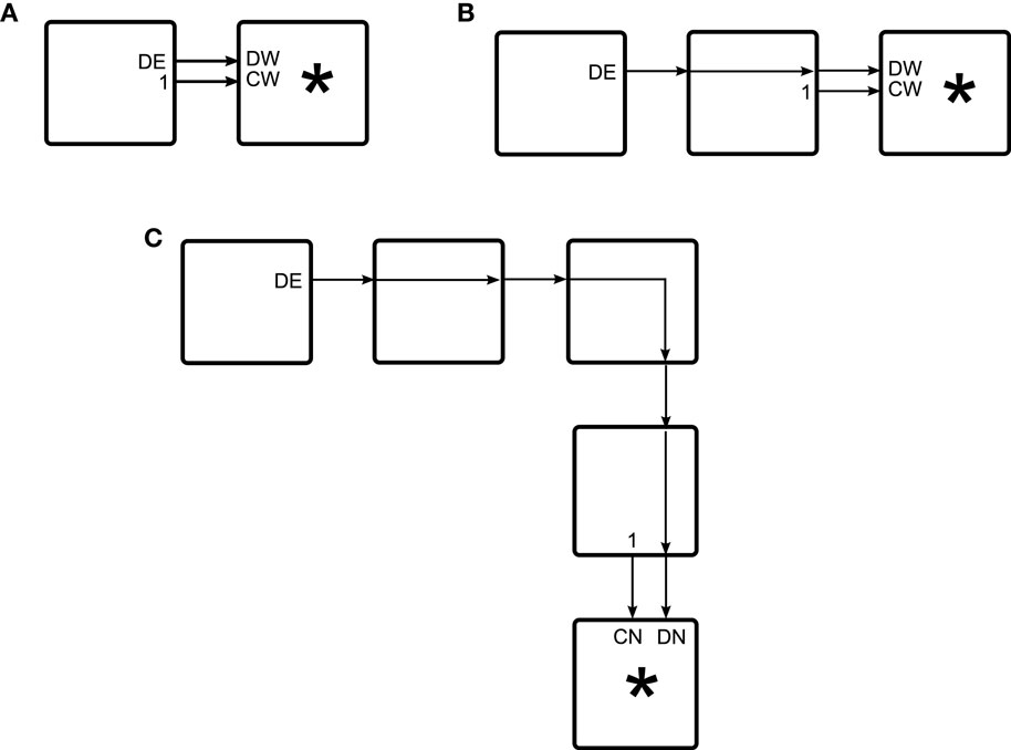
Figure 1. Examples of C-mode operations within a Cell Matrix. (A) shows a single source cell (on the left) configuring an adjacent target cell (labeled “*”). (B) shows a source cell configuring a non-adjacent target cell “*” via an intermediary cell adjacent to both the source and the target. (C) shows a source cell configuring a more remote target cell via a number of intermediate cells. The source cell’s DE output is be generated by other cells (not shown), and supplied to the source cell for transmission to the target.

From the above description, it should be no surprise that a cell is a relatively expensive piece of hardware: to tile a 2D matrix with cells connected with von Neumann neighborhoods requires 4-sided cells, thus each cell’s truth table contains 16 rows (16 combinations of 4 D inputs) and 8 columns (4 D and 4 C outputs), or 128 bits of storage per cell. With additional logic, this means a single cell contains roughly one thousand transistors, yet this single cell may be acting as nothing more complex than a simple wire, conveying a single bit of data from one of its sides to another. This raises an important question: why work with an architecture that requires spending thousands of transistors to create a simple wire?

The answer is that the resulting wire is much more than just a wire: it is an element that, in addition to acting as a wire, can be analyzed, relocated, modified, isolated; and whose constituent cells can be used to analyze, relocate, modify, or isolate nearby elements (Macias, 2011).

One area where this comes into play is in bootstrapping an initial configuration of cells – a task especially relevant for self-assembled systems, since self-assembly usually supposes identical elements whose differentiation will occur post-assembly.

Bootstrapping requires loading initial truth tables into each of a set of cells. On other reconfigurable devices, this may be accomplished, for example, by serially loading in each truth table. The device would contain circuitry for directing each truth table’s bits into the appropriate cell’s configuration memory, according to a pre-defined ordering. Alternatively, the serial configuration information can include a cell ID with each configuration bitstream, thus directing the device’s configuration circuitry to load the bits into the proper cells (Soni et al., 2013).

One disadvantage of these approaches is speed: configuration information is supplied sequentially, and thus the length of the total configuration stream increases as the number of configured elements increases. Another potential disadvantage is that a rigidly defined boot sequence may be wasteful time-wise if only certain cells are in need of configuring.

On the Cell Matrix, bootstrapping works very differently, as there is no pre-defined bootstrap mechanism for loading a collection of truth tables into a set of cells. Instead, the circuitry for loading these configurations is itself built from cells (which must themselves be configured, via another bootstrap mechanism, which is itself built from configured cells; and so on). Note that this process is reminiscent of the use of the term “bootstrapping” in describing the startup process for early programmable computers (Buchholz, 1953).

Here again, it could at first seem to be a disadvantage that there is no pre-existing bootstrap mechanism in the Cell Matrix; and in terms of quickly loading a configuration from scratch, this does complicate the process by requiring additional steps. But in terms of flexibility, it is actually a significant advantage over a fixed bootstrap mechanism. For example, bootstrap circuitry can be built in whichever regions of the matrix require bootstrapping; multiple bootstrap circuits can be built and operated in different parts of the circuit, at different times (or simultaneously), as dictated by the particular task at hand. Moreover, if a desired configuration employs numerous identical (or systematically differentiated) copies of a smaller sub-circuit, a custom bootstrap circuit can be designed to perform massively multiple simultaneous configurations (Macias, 2011).

This ability to design a bootstrap circuit from scratch – a unique aspect of the Cell Matrix relative to most other reconfigurable systems – will play a central role in the present work, as it provides a mechanism for dealing with potential complications in the manufacture of a large-scale reconfigurable system via self-assembly.

3. Self-Assembly

Whereas much of today’s manufacturing is performed via externally directed assembly (for example, in a factory), self-assembly creates a system that, once built to a certain initial stage, begins acting autonomously to further construct itself (Whitesides and Grzybowski, 2002). To a large degree, this idea is inspired by examples from the natural world. For example, a 6-mm seed contains the instructions and machinery necessary to grow into a sequoia tree 100 m high and 9 m in diameter (Efloras, 2015).

In biological systems, self-assembly needs to proceed under a wide range of possible conditions. For example, the orientation of the seed in the ground cannot be predicted, yet the initial sprout must grow upwards, to emerge into sunlight. If there is a rock or other obstruction above the seed, the sprout may work its way around the obstruction until it can grow through soil to reach the surface, or it may break through the obstruction (for example, an area of pavement) if routing around it is not feasible. The mechanics for these operations – for assessing and responding to the situation – must also be present within the seed.

Examples of self-assembled systems abound in nature, and include the development of living systems as well as the growth of inorganic crystals. Human-made examples include self-assembly of mechanical structures (Mao et al., 2002); self-assembly of 3D polyhedra (Leong et al., 2007); and self-assembly of electronic circuits (James and Tour, 2005). Algorithmic work on self-assembly includes directed self-assembly (Grzelczak et al., 2010) and applications to nanofabrication (Ozin et al., 2009), as well as research into autonomous self-repairing/differentiating systems on a Cell Matrix (Macias and Athanas, 2007).

Self assembly offers the following advantages over externally directed assembly:

• the assembly process itself is effectively contained within the system being assembled, meaning simple control structures can first be self-assembled and used to build more-complex control structures, which can then be used to control further self-assembly;

• being primarily self-contained, a self-assembling system can be placed effectively anywhere inside its growth medium, as opposed to needing to be placed near specifically located external control structures; and

• multiple copies of a self-assembling system can be installed throughout a growth medium, allowing for parallel assembly of multiple copies of the system. This is advantageous for fast assembly, as well as for situations where some of the systems may not assembly to their desired end state (for example, when defects are present).

There are also some disadvantages to the self-assembled approach, including the following:

• a self-assembled system may be more complex, since necessary mechanisms for controlling the assembly process may need to be embedded in the self-assembling units;

• since the assembly proceeds autonomously, process errors – defects, misconnections between units, etc. – need to be detected locally and handled appropriately, without external intervention; and

• lacking centralized control, global tasks must be re-framed in a way that supports their execution using only local information.

The present work explores a self-assembled system for implementing a Cell Matrix (Macias and Durbeck, 2013). The Cell Matrix was chosen for the following reasons:

• The Cell Matrix is an extremely fine-grained system: each cell is a simple 4-input 4-output logic block, suitable for implementing basic functions such as an AND gate, an inverter, a 1-bit adder, or a 2-1 selector. This presents a relatively simple initial build target for a self-assembling technology, yet once assembled, more-complex elements (such as flip flops, ALUs, or CPUs) can be built from a collection of these fine-grained cells.

• Once a matrix of simple cells has been built via self-assembly, complex control structures necessary for further self-assembly can be built from these simple cells via configuration of the already-assembled simple cells, rather than via physical assembly of more-complex blocks.

• Details of these control structures can be changed without modifying the underlying self-assembly process. To implement, for example, a new algorithm for managing differentiation of identical coarse-grained blocks, one need not change the basic simple cell definition; rather, one simply uses the same cells in a different configuration.

• Since a central feature of the Cell Matrix architecture is the ability of cells to interrogate and modify nearby cells, it is feasible to build circuits (again, from simple cells) that can check nearby cells for defects, and re-configure circuits to avoid those defective cells. This means that as complex control systems are being built, in-system testing can be performed and faulty cells identified and worked-around as the control systems expand.

Another advantage of a Cell Matrix over other possible target architectures is that its architecture is flat – there is no inherent hierarchy among the cells of the matrix. This has significant advantages in terms of scalability: since all cells are identical, simply adding more cells to the edge of an existing matrix creates a larger matrix. With proper management of configuration tasks in such a system, not only will the hardware scale well, but the algorithms involved in managing the system can exhibit better than O(n) performance, by allowing multiple control circuits to be built throughout the matrix. This can also help with re-framing global tasks (such as differentiation of identical blocks into specialized units) into distributed, parallel, local operations.

3.1. Key Challenge to Be Addressed

Despite the advantages of a Cell Matrix as a build-target, its simplicity presents a significant challenge with respect to how cells are placed within the matrix. Each cell has a natural orientation: for a 2D 4-sided cell, its sides are addressed internally as North, South, West, and East (N, S, W, E respectively). In order for two cells to interact correctly with each other – for example, for one cell to correctly configure a neighboring cell – these cells need a common sense of orientation. If cell A intends to send data out its eastern edge to cell B (which is located on A’s eastern edge), cell A needs to know which of cell B’s edges is adjacent to cell A’s eastern edge. If cells A and B are oriented identically, then cell B’s western edge will sit adjacent to cell A’s eastern edge. But if cell B is rotated relative to cell A’s orientation, then it may be (for example) that cell B’s northern edge is adjacent to A’s eastern edge (Figure 2). These orientation differences will affect how cell A must configure cell B.

FIGURE 2

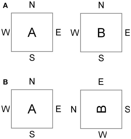
Figure 2. Effect of dis-orientation on inter-cell behavior. In (A), cells A and B are oriented the same, so cell A can send data to B’s western edge. In (B), cell B is rotated relative to cell A, so cell A has access only to cell B’s northern edge.

The problem is similar to trying to build a circuit using ICs whose pins have unknown connections to the chip’s internal circuitry (but where one still knows which pins are inputs and which are outputs). To connect the output of one IC to the input of another, one needs to know which pins correspond to which functions of the chip. If that mapping is unknown, then the chips cannot reliably be connected together without first somehow determining that mapping.

4. Materials and Methods

This issue of mis-oriented cells is a particular concern with self-assembly, since some processes may not guarantee the physical orientation of blocks as they are assembled into a larger structure. There are at least three approaches to deal with potential mis-orientation of elements in a self-assembled system:

1. correct the physical orientation of blocks as they are being assembled, so that there is no dis-orientation in the final assembly;

2. endow the blocks with the ability to sense their own orientation, and have them re-adjust their internal wiring so that their faces are effectively oriented normally; or

3. allow the physical matrix to be assembled with mis-oriented cells, but then somehow determine post-manufacture what each cell’s orientation is, and use that information to adjust how the matrix is used.

The first approach may be feasible by, for example, weighting the faces of each block unequally, so that the blocks orient themselves as they fall slowly through a viscous liquid. Alternatively, ferrous coatings on certain faces could help orient the blocks in the presence of a strong magnetic field, applied along one axis of the intended assembly (Tousley et al., 2014). Some work has been done using chemically directed self-assembly (Diehl et al., 2002). While these approaches address the problem of properly orienting elements, they are somewhat contrary to the spirit of self-assembly, falling more in the realm of directed assembly (Grzelczak et al., 2010). Moreover, they require adjusting the physical design of the building blocks based on this particular issue. This runs contrary to the goal of having fixed hardware and modifying behavior only through software changes.

The second approach seems straightforward. One can re-design the basic Cell Matrix cell’s architecture to include orientation-detecting circuitry, as well as an intra-cell routing network to change which sides are connected to which parts of the cell’s internal circuitry. Following assembly, a one-time, post-manufacture orientation step can be performed, during which the cells effectively re-orient themselves (not physically, but by changing their internal notion of sidedness). This could work well, but requires a significantly more complex cell architecture. Moreover, it violates a fundamental principle of Cell Matrix design, which is to maintain the simplest possible cell architecture, and introduce greater complexity by building circuits from the cells themselves.

The third approach is very much in the spirit of the Cell Matrix, being based on the concept of introspective circuitry, running potentially in parallel at multiple sites throughout the substrate. Moreover, because it is based on analysis performed from within the system itself, it requires correctly-functioning hardware adjacent to the locations where problems (mis-­orientation) are being detected, analyzed, and corrected. On many platforms, this is a classic quandary: how to analyze potentially faulty hardware using circuitry built on hardware that is itself potentially faulty. With its distributed, localized control, its ability to read and write configuration information, and the interchangeability of the source and target of configuration operations, the Cell Matrix is well suited for exactly this kind of situation.

While each approach has its merits, it is this third approach that is employed in the present work. This choice is motivated by the goal of taking an existing self-assembly technique (self-assembling self-folding polyhedra) and using it to implement previously defined cells (constituents of a Cell Matrix). Approach 1 requires re-design of the former, which approach 2 requires re-designing the latter.

The approach will be detailed in three pieces:

1. detection and handling of a single mis-oriented cell;

2. linear (O(n)) detection and handling of mis-orientation in a 2D region of cells; and

3. sublinear (O($\sqrt{(}n)$)) detection and handling of mis-orientation in a 2D region of cells.

4.1. Detection and Handling of a Single Cell’s Orientation

Detecting the orientation of a cell adjacent to a working cell is straightforward. Consider the four possible situations shown in Figure 3. In each case, the cell’s truth table has been loaded with the equation DN = S, which copies data from its southern D input to its northern D output. In the leftmost case (where the cell is oriented as expected), the cell behaves as expected; but in the other cases (where there is a mis-orientation of the cell), the cell’s behavior is different from what was expected.

FIGURE 3

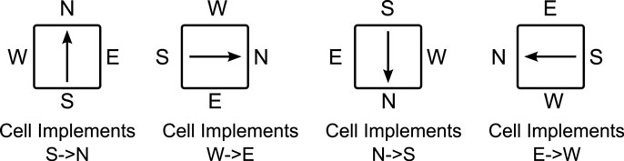
Figure 3. Four possible orientations of a cell. The cell is configured with the equation DS → DN, but depending on its orientation, the actual function may be DS → DN, DW → DE, DN → DS or DE → DW.

Even though a cell may be mis-oriented, it can still be programed from any chosen side: the problem is that the program loaded into a cell will likely act differently from what is expected. Fortunately, it is this very fact that makes it possible to detect a cell’s orientation.

For example, suppose one has access to the actual western edge of a target cell, as shown in Figure 4. Here, the cell labeled “*” is able to be configured in a controlled way (i.e., its orientation is known and has been corrected for). “*” may wish (under the direction of a larger, multi-celled circuit) to use this neighboring target cell to send information to a more remote cell, so it will try to load the truth table corresponding to DE = W (which configures a cell to send data from its western input to its eastern output) into the target cell. But depending on its orientation, the target cell will end up in one of the four configurations shown. Only one of these is the desired configuration: the other three read data from a cell other than “*.”

FIGURE 4

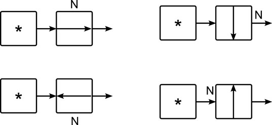
Figure 4. Effect of dis-orientation on a multi-cell circuit. Two cells are used to build a wire, but depending on the orientation of the cell on the right, the resulting circuit may not function correctly. In the above examples, only the first circuit works correctly as a wire.

Figure 5 shows the results of configuring a different truth table: one for DW = W (which echos data from the cell’s western input back to its western output). As can be seen, only in the first case – where the cell is oriented as expected – results in a circuit whose input and output are accessible from cell “*.” Figure 6 shows four target cells, each in a different orientation, each configured to allow access from cell “*.” In Figure 6A, the normally oriented target cell is configured with the truth table DW = W. In Figure 6B, the target cell is configured with the truth table DS = S; in Figure 6C, the cell is configured with DE = E; and in Figure 6D the equation is DN = N.

FIGURE 5

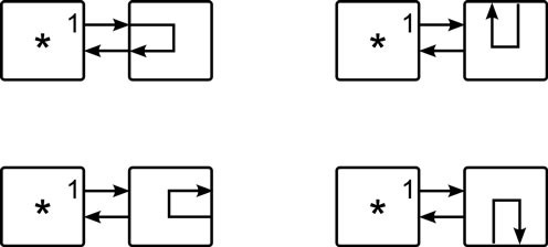
Figure 5. Configuring a cell with the equation DW → DW produces one of four circuits, depending on the orientation of the cell on the right. Only a normally oriented cell will produce a circuit that echos its DW input.

FIGURE 6

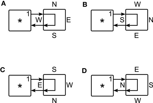
Figure 6. Four possibilities for reading an echo from a neighboring cell. Each part (A–D) shows a different orientation of the cell on the right. In each case, there is a unique configuration of the cell that will produce an echo.

Since cell “*” can write and read data form the target cell on its right, it is possible for it to determine the orientation of the target cell as follows:

• configure the cell with DW = W, then send a bit pattern out cell “*”’s eastern output, and look for the same bit pattern to be returned by the target cell. If the sent pattern is detected, then the target cell is oriented with North to the top;

• configure the cell with DS = S; a successful echo means the cell is oriented with North to the right;

• configure the cell with DE = E; a successful echo means the cell is oriented with North at the bottom;

• configure the cell with DN = N; a successful echo means the cell is oriented with North at the left.

Note that if none of these tests returns the expected data, then there is an error in the cell’s behavior. Assuming there are no defects, one of the above tests should reveal the target cell’s orientation.

The above technique allows determination of a single target cell’s orientation. This is of little use though unless the target cell can subsequently be used despite its mis-orientation. This is straightforward in practice: given a Boolean equation expressing each side’s output in terms of inputs from each side, a permutation of the sides {N, S, W, E} → {W, E, S, N} will compensate for a 90° clockwise rotation of the cell.

As an example, consider the equation DS = WN + WE (which specifies that the southern output is the logical OR of two product terms: one being the AND of the west and north inputs; the other being the AND of the west and east inputs). Under a 90° clockwise rotation of a cell, the northern edge now faces east, the eastern edge faces south, and so on. The permutation can be described as N → E, E → S, S → W, and W → N. Under this permutation, the equation DS = WN + WE translates to DE = SW + SN. In other words, by loading this latter equation into the rotated cell, the cell will act the same as a properly oriented cell whose program is DS = WN + WE. Rotations of more than 90° are handled by successively applying permutations for each 90° rotation. Counter-clockwise rotations are treated by considering their corresponding clockwise rotation.

4.2. Detection and Handling of a 2D Region of Cells

Orienting (and bootstrapping) an entire 2D region of cells requires a sequence of steps, beginning with a small initial set of cells (with known orientation), which comprise circuitry for analyzing other regions of the matrix (using the steps described above). This requires some intermediate machinery though.

To utilize the above algorithm for determining a target cell’s orientation, it is necessary to have access to the target cell’s C and D inputs and outputs. While cells in the Cell Matrix have direct access only to their immediate neighbors, it is relatively straightforward to use a set of cells to gain access to a non-adjacent cell, using a construct called wire building (Macias and Durbeck, 2013).

Wire building begins by having an original cell configure a neighboring cell in such a way that the neighbor will configure one of its neighbors (which is non-adjacent to the original cell). This is straightforward, and works well for configuring cells that are almost adjacent. Using this to configure, more-remote cells is not practical though as it requires repeated forward-and-backward steps (similar to solving Towers of Hanoi): the time complexity for a cell n steps away is O(2ⁿ).

Practical wire building requires cooperation between cells so as to effectively reposition the region of cells that are directly accessible. This is accomplished by first configuring a 2 × 1 (sometimes 3 × 1) column of cells, in such a way that they can be used to configure an adjacent column identically. The pair of columns can then be used to configure a third column, and so on. This 2 × n structure is called a multi-channel wire, and can be extended in linear time: three fixed-length programing cycles per cell extension. Using a 3 × n wire allows the wire to carry a break signal, which can be used to retract the wire.

Building these columns that comprise a multi-channel wire involve sending repeated sequences of 1’s and 0’s into the wire so as to control the target cell’s C and D inputs, causing it (and nearby cells) to configure other cells, thus extending the wire. This is easily controlled by simple circuits, allowing circuits within the matrix to extend control over non-adjacent cells. Additional sequences also exist for building corners (comprising 12 programing cycles), and, combined with sequences for building linear wires, allow movement throughout the matrix in linear time. Further details of these sequences can be found in Macias and Durbeck (2013), as well as in a series of online tutorials (Cell Matrix Corporation, 2013).

While wire building has been well-understood for many years, trying to deploy these circuits in a dis-oriented matrix poses new challenges: each cell must be analyzed, and any rotation compensated for, before it can be used to configure other cells. This is achieved by incorporating the techniques from the previous section during the sequencing process.

Configuration of a 2D region is likewise accomplished by successive application of single-cell orientation detection and correction, interspersed throughout a standard bootstrap protocol as described in Macias (2011). For a m × n region of cells as shown in Figure 7, a typical protocol proceeds as follows:

1. A 2 × n − 3 (i.e,. two-channel) wire is built across the top two rows of the region (initiated from the two cells for which direct access is available);

2. a 2 × 2 corner is built near the upper-right corner of the region, allowing;

3. the two-channel wire to extend further to the south;

4. as this wire extends, target cells are configured to the east of the wire’s head;

5. after reaching the bottom of the region, the rightmost column of the region has now been configured with the intended final target configurations.

FIGURE 7

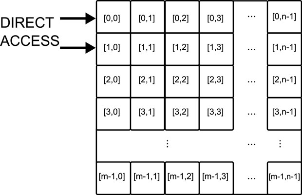
Figure 7. Layout of cells within a matrix. Given direct access to cells [0,0] and [1,0], indirect access is available to cells [0,1] and [1,1].

The wire is then broken at its beginning (the cells over which direct access is available), and the above steps repeated but the initial wire is extended to a length of n − 4. This allows the second column from the right to be configured.

This repeats until all but the leftmost 2 columns have been configured. These are then configured in the front of a southern-extending wire. Finally, the upper-left 2 × 2 region is configured using a one-off set of sequences.

At the conclusion of this entire set of configuration sequences (a so-called “super-sequence”), the entire m × n region will have been configured as desired. While this works well for modest-sized regions, the time complexity grows like O(nm), which makes it impractical for configuring extremely large regions. To bootstrap in a way that scales well with the number of cells, it is necessary to take advantage of the inherent parallelism of hardware, to not only achieve multiple simultaneous configurations, but to increase the multiplicity of configuration sites as the number of configured sites increases.

4.3. Sublinear Handling of a 2D Region

The linear configuration time of the process described above is impractical for large-scale configuration. For certain types of circuits, it contains a high-degree of homogeneity, parallel configuration can significantly improve this situation. For example: a regularly tiled neural network; a cellular automata-based processor; and a distributed simulation of heat flow each involve circuity comprised of a large, regular collection of identical circuits. Configuring a Cell Matrix with these repeated patterns of digital circuitry can be done efficiently by first building a parallel configuration circuit, and then using that circuit to configure the desired target cells in parallel.

Circuits that employ this kind of parallel operation are called Medusa Circuits (Macias and Durbeck, 2016). To a first order, a Medusa circuit is simply a multi-channel wire with multiple heads (Figure 8). By copying D and C inputs to multiple cells instead of a single cell, multiple cells can be configured in parallel. This approach is well suited for configuring a large number of copies of identical circuits by building multiple wires orthogonal to the Medusa wire. Thus, once a one-dimensional wire has been built (which takes O(n) for a wire with n heads), it can be used to build n orthogonal wires, extending those in parallel in a fixed amount of time (independent of n).

FIGURE 8

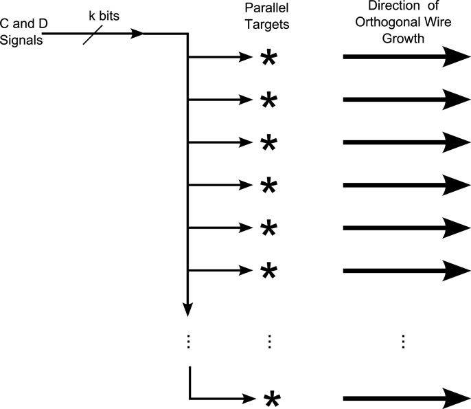
Figure 8. Medusa Wire. C and D information is sent into the wire from the upper left, and delivered in parallel to each wire head, thus allowing parallel configuration of the target cells marked “*.” The wire itself may be 2-, 3-, or more-generally k-channeled, depending on how it is to be used. Typically a Medusa wire is used to build and extend wires orthogonal to the major axis of the Medusa wire itself.

Like simple multi-channel wires, Medusa wires have also been well-understood for some time, and their use for parallel configuration is nothing novel. In the present situation though, where dis-oriented cells must be contended with, there is a bit of a catch-22:

• to minimize configuration time, configuration of multiple regions should be done in parallel; but

• in order to deal with the dis-orientation (which may be different from cell to cell), each cell being configured must be analyzed, and different configuration information (rotated based on the degree of rotation of the target cell) must be delivered to different cells.

These requirements would seem to be at odds with each other: how can parallel operation be maintained when different regions require different configuration instructions? The solution is to move part of the processing so that it is done locally, next to each head of the Medusa wire. This requires some care.

Figure 9 shows the circuitry used to locally manage dis-orientation of cells. There are two separate but related tasks to be accomplished while extending a wire:

1. run a series of tests, checking each possible orientation of the target cell, and record the true orientation of the cell; and

2. select and apply the appropriate configuration string for the discerned orientation.

FIGURE 9

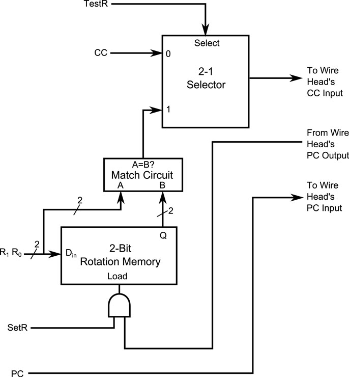
Figure 9. Control circuit for local management of cell dis-orientation. The PC and CC signals are normally routed to the D and C inputs of the target cell, as usual. R₁ and R₀ code one of four possible rotations. SetR is used to record the result of a successful orientation test on a target cell. TestR is used to block the CC signal unless R₁R₀ match the saved R₁R₀ that were recorded when SetR was asserted. By pairing configuration information with R₁R₀ and TestR, bitstreams will be processed or ignored locally, based on the results of prior analysis.

The circuit in Figure 9 – which sits at the head of each wire coming from the Medusa wire – manages both of these tasks. The PC line carries bidirectional information to each target cells’ D input and output. This transfer occurs regardless of any other signals related to the circuit. The CC line drives the target cell’s C input, provided TestR is not asserted. Thus, PC and CC can be used to load test patterns into the target cells; to stimulate the test circuits; and to read the target cells’ responses.

Recall that to determine a cell’s orientation, a feedback circuit is loaded into the cell, a signal is sent to the cell’s D input, and an echo is listened for. During the echo test, the SetR signal is asserted, while R₁R₀ carry a coded representation of the rotation currently being tested for. If an echo is detected on the PC signal (coming from the target cell), it will cause the Rotation Memory to record the current values of R₁R₀; otherwise the memory is left unchanged. Thus, at the conclusion of all 4 tests, the true rotation of the target cell will be saved in the Rotation Memory of each wire being used to configure a target cell. However many wires are being used, it requires only 4 tests to set the Rotation Memory for each wire.

Following this diagnostic step, the desired configuration information is then sent to the target cells, four times: once for each possible rotation. Along with the configuration information, the corresponding R₁R₀ (indicating the rotation ofthe current configuration information) is sent, and the TestR signal is asserted. With TestR = 1, the CC signal is only allowed to pass to a target cell if the Rotation Memory matches the current value of R₁R₀. Thus, all four possible configuration strings are delivered – one at a time – to all cells in parallel, but each cell will only make use of the one corresponding to that cell’s orientation.

Thus, the circuit in Figure 9 restores the ability to configure multiple target cells in parallel, which tailoring the configuration to each cells particular orientation. The added cost is a small (14 × 13 cells) additional circuit near the beginning of each wire. This changes the time complexity of configuring a square region of n cells from linear (O(n)) to sublinear (O($\sqrt{(}n)$)).

5. Results

The proposed approach to managing a dis-oriented array was implemented, simulated, and show to work as expected, for single-cell, multi-cell, and parallel operations. Verifying this required the following steps:

1. a simulator of the Cell Matrix needed to be modified to simulate mis-oriented cells throughout the matrix;

2. the unusability of this matrix was verified by performing simple configuration operations and observing the incorrect behavior;

3. the ability to detect orientation was then tested in different regions of the Matrix by running the prescribed tests and observing target cell responses;

4. these tests/observations were incorporated into a 2D bootstrap sequence, and used to produce an orientation map for the entire 2D region, and the discerned orientations were confirmed to match the simulated dis-orientation;

5. orientation test/correction circuitry was designed, implemented in cells, and loaded into the simulator, and its behavior was verified; and

6. a Medusa wire was built, with multiple copies of this test/correction circuitry (one per head), and successful parallel extension of the wires – despite random orientations of the underlying cells – was observed.

5.1. Simulation

The standard Cell Matrix simulator is normally used interactively by a user, but was modified for this work to allow inputs to be driven from/outputs delivered to an analyzer program running on a PC, thus allowing the above algorithms to be driven from high-level code.

The simulator itself employs an internal cell-to-cell connection map, in order to allow various dimensions and topologies to be used with a single set of simulator code. During the execution of the simulator, outputs are conveyed to inputs by consulting this connection map, discovering which cell/input is connected to a changed output, and adding the corresponding (new) input change to an event queue. This simulates signaling from cell to cell as the simulation progresses.

Normally, this map connects together nearest neighbors in the expected way: N–S and W–E. For these experiments, a random orientation was assigned to each cell in the simulated matrix, and the connection map was modified accordingly to reflect the local dis-orientations. As a result, the simulated matrix was effectively unusable: configuring a cell with the equation “DN = S” could result in any of the 4 configurations shown in Figure 3.

Since initially the entire matrix is dis-oriented, the first steps of the analysis algorithm must be performed on an external system (in this case, the analyzer program). Subsequent steps utilize the cells themselves, as they are (effectively) re-oriented.

5.2. Orientation Determination

The analyzer program was used to apply the above algorithm to discern the orientation of each cell, beginning with edge cells, and using that information to move further into the interior of the matrix, sweeping out a 2D pattern using the bootstrap sequence described above.

While cells were analyzed, the discerned rotations were conveyed to the analyzer program, and written to a file, which was compared to the simulator’s own orientation map. Figure 10 shows the resulting map, which was randomly generated by the simulation code and used to direct internal cell I/O traffic. This was for a 16 × 16 matrix. Each digit corresponds to a single cell, and its value indicates the cell’s orientation in terms of how many clockwise 90° turns the cell has undergone from its normal orientation.

FIGURE 10

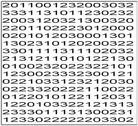
Figure 10. Orientation map for test run. A 16 × 16 simulated matrix was given random orientations, to allow testing of the orientation-detection algorithm. Each digit corresponds to a single cell; the value shows the number of 90° clockwise turns of the cell from its normal orientation.

This map was then subsequently discovered by the analyzer algorithm, which printed it at the end of its analysis, and it was confirmed to match the simulator’s own orientation information. Thus, successful discovery of cell orientation was confirmed, albeit from an inherently sequential, O(n) algorithm.

5.3. Adaption to Dis-Orientation

No additional work was required to test the approach’s ability to handle dis-oriented cells: in order for the detection algorithm to work throughout a 2D region, it was necessary for the circuitry to construct wires, corners, and other circuits throughout the 2D region. This is not possible unless the system is able to successfully compensate for each cell’s random rotation. Successful completion of the above orientation map confirms not only the ability to detect orientation but also the ability to utilize cells despite their mis-orientation.

5.4. Parallel Algorithm and Scalability

Finally, the fully parallel algorithm was tested, using local copies of the orientation detection/handling circuit (Figure 9). Figures 11A–E show the graphical output from the simulator while it was working on three regions in parallel.

FIGURE 11

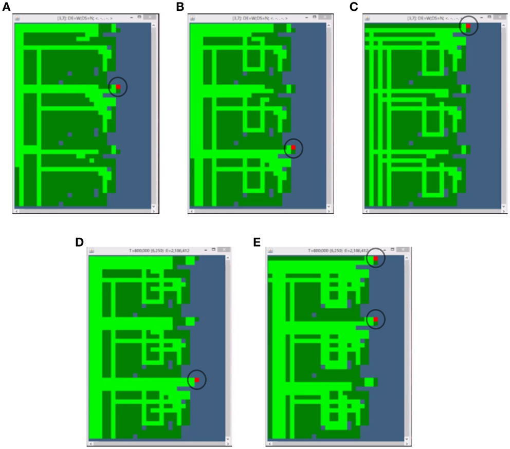
Figure 11. Orientation Test Results. These images show the graphical output from the simulator running this algorithm on 3 regions in parallel. In (A), a target cell in the second region (from the top) is being configured, because its orientation corresponds to the currently delivered configuration string (the target cell is circled in each figure). In (B), the target cell in the third region is configured; and finally, the target in the first region is configured in (C). In (D), a new target in the third region is configured. In (E), a pair of targets – one in each of the top two regions – are configured, as they each have the same orientation as the delivered configuration string.

If Figure 11A, a target cell (circled in the figure) is being configured in the middle region of cells. The configuration information is being delivered to target cells in each of the three regions, but only the middle region is allowing the CC signal to reach the target cell (based on that region’s saved orientation information).

In Figure 11B, it is the target in the 3rd region that is being configured, while the CC signal to the top two regions is blocked. Then in Figure 11C, the target in the top region is configured. There was also a 4th configuration string sent (corresponding to a 4th orientation) that was not used for any of the regions in this step.

In Figure 11D, the orientation of the next target cell in the lower region now matches the orientation of the delivered configuration string, so the CC signal is routed to the target cell only in that region, while it is blocked in the first two regions. In Figure 11E, the orientation of the target cell in the upper two regions matches the delivered string’s orientation, and thus the CC signal is routed to the target cell in both of those regions. Here, we thus have two targets being configured simultaneously.

In general, roughly 25% of target cells will be configured in parallel (assuming a uniform distribution of cell rotations), though which particular cells will be configured at each step is effectively unpredictable.

Subsequent testing was done on 32 parallel wires, and successful operation was confirmed via the simulator’s graphical output. An online video is available at (Cell Matrix Corporation, 2015).

Table 1 shows the number of timesteps required for re-orienting and configuring an n × n region of blocks in this way.

TABLE 1

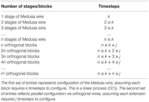
Table 1. Number of configured blocks vs. total number of timesteps required for configuration.

For a square array of n × n blocks, this means it takes roughly n × k + n × j = n × (k + j) timesteps, where k and j are independent if n. In other words, configuring n² blocks has a time complexity of O(n); or, equivalently, configuring n blocks has a time complexity of O($\sqrt{(}n)$) This is far superior to O(n) (linear performance), and makes tractable the question of configuring, say, 10¹⁸ blocks (which, under this approach, requires the same time-order as linearly configuring 10⁹ blocks).

6. Conclusion

As fabrication of large-scale reconfigurable systems moves from traditional top-down assembly to next-generation bottom-up self-assembly, a number of technical challenges will arise. Given the lack of centralized control in a self-assembly process, new hurdles are anticipated, including the issue of un-regulated orientation of building blocks prior to their inter-connection. While circuitry can be added to such blocks specifically for detecting and correcting their orientation, this complicates the design, potentially increasing the likelihood of defects and failures, as well as further complicating the assembly process. In general, adding task-specific features by modifying the hardware design may produce a more-optimal solution for that given task, but at the expense of introducing non-general-purpose hardware. If extremely rapid orientation/assembly were a concern, this might make sense; but in general, incorporating only hardware that can be re-used for whatever purpose is desired post-assembly avoids over-complicating the cell design and diminishing the cell density in the matrix.

While the present work is potentially useful for the task at hand – that of orienting a collection of cells – its significance is something beyond that particular goal. The real significance of this work is to demonstrate – by specific example – how system-level problems that might otherwise be solved by the use of external machinery can instead be solved using distributed, locally acting, internal circuits that are built on-the-fly. This echoes themes found in similar works (Durbeck and Macias, 2002; Macias and Athanas, 2007; Macias, 2011). There are two underlying concepts here:

1. using a bootstrap-style approach to problem solving, wherein a large-scale problem is solved for a small subset of cells, which are then used to solve the problem on a larger set, and so on. This approach can be used to address, for example, the challenge of building a circuit to detect faults when the substrate containing the test circuit may itself be faulty (Macias and Athanas, 2007); and

2. in many large-scale systems, increasing the system size increases the difficulty of managing the system; but in a system that has an inherent self-duality – where cells can interchangeably be the controller of or the target of configuration operations – an increase in the ability to control the system’s complexity can accompany the increase in the complexity itself, thus making it feasible to scale the system to an arbitrarily large size.

Even though this entire process may be driven by circuitry external to the reconfigurable substrate itself, and the system-wide clock represents an external signal, this external driver is a small, fixed-sized/fixed-complexity piece of the entire solution. The key innovation of this work is that critical pieces of the process – the pieces that represent an ever-increasing workload as the system scales – are handled from within the substrate itself, being developed and deployed as more and more of the substrate is made usable.

7. Future Work

Presently, the basic parallel detection and effective re-orientation of 2D cells has been tested using a cell-level simulation, but much of the control of the circuitry has been done above the cell-level, via a program running outside the simulator. A fully self-contained version of this work – comprised entirely of digital circuitry made from (simulated) cells – remains to be built. This is a fairly mechanical process though laborious process and is not expected to add to the overall significance of this work. As a further proof-of-concept though, it is a step that should still be taken.

The present work allows efficient determination of cellular orientation, providing information that can be used by configuration circuitry to effectively re-orient dis-oriented cells. An alternate way of utilizing this information is to store orientation data in a small set of cells near each block of circuitry; assigning local addresses to these blocks thus making them row/column addressable; and using that stored information to adjust configuration strings on the fly. This would effectively place an intermediate layer between the target circuitry and the low-level cells of the Matrix, thus reducing density and, to some degree, speed, but in exchange for being able to act as if the cells are all normally oriented.

Yet another approach to efficiently managing the cell-level dis-orientation is to utilize super self-duality, wherein a collection of cells are used to implement a circuit that acts like a single cell (a “supercell”). This shifts the challenge of re-orienting cells to a one-time task during the construction of each supercell.

While these and other embellishments will be explored at a future date, none of them would seem to add significantly to the central tenet of this work, which is that there is benefit to shifting control from a single centralized external location to numerous distributed, internal sites, specifically in a way that allows the control to scale along with the scaling of the problem size itself.

Author Contributions

LD was involved in the early stages of this research, particularly those areas related to autonomous operation of circuits in the given substrate. CT was involved in research related to self-assembly, and the particular question of cellular orientation. CT also contributed significantly to the editing of the manuscript. NM was responsible for developing and implementing the specifics of the presented algorithm, and wrote the initial draft of the manuscript. All authors have reviewed the manuscript and agree to be accountable for all aspects of the work.

Conflict of Interest Statement

The authors declare that the research was conducted in the absence of any commercial or financial relationships that could be construed as a potential conflict of interest.

The reviewer Malte Harder and the handling Editor Daniel Polani declared a past supervisory relationship with each other, and the handling Editor states that the process nevertheless met the standards of a fair and objective review.

Funding

This work was supported by the Cross-Disciplinary Semiconductor Research (CSR) Program award G15173 from the Semiconductor Research Corporation (SRC).

References

Baumgarte, V., Ehlers, G., May, F., Nückel, A., Vorbach, M., and Weinhardt, M. (2003). Pact xppa self-reconfigurable data processing architecture. J. Supercomput. 26, 167–184. doi: 10.1023/A:1024499601571

CrossRef Full Text | Google Scholar

Blodget, B., James-Roxby, P., Keller, E., McMillan, S., and Sundararajan, P. (2003). “A self-reconfiguring platform,” in Field Programmable Logic and Applications,13th International Conference, FPL 2003, Lisbon, Portugal, September 1-3, 2003 Proceedings, eds P. Y. K. Cheung, and G. A. Constantinides (Springer), 565–574.

Google Scholar

Buchholz, W. (1953). The system design of the IBM type 701 computer. Proc. IRE 41, 1262–1275. doi:10.1109/JRPROC.1953.274300

CrossRef Full Text | Google Scholar

Cell Matrix Corporation. (2013). Cell Matrix Course, Wire Building. Available at: https://cellmatrixcourse.wordpress.com/2013/06/26/u008-2-channel-wires/ [accessed December 13, 2015].

Google Scholar

Cell Matrix Corporation. (2015). Parallel-Differentiating Medusa. Available at: https://www.youtube.com/watch?v=GNLJ-0mmhqA [accessed December 14, 2015]

Google Scholar

Cooper, K. D. (2014). Making effective use of multicore systems a software perspective: the multicore transformation (Ubiquity symposium). Ubiquity 2014, 1–8. doi:10.1145/2618407

CrossRef Full Text | Google Scholar

Diehl, M. R., Yaliraki, S. N., Beckman, R. A., Barahona, M., and Heath, J. R. (2002). Self-assembled, deterministic carbon nanotube wiring networks. Angew. Chem. Int. Ed. 41, 353–356.

Google Scholar

Durbeck, L. J., and Macias, N. J. (2002). “Defect-tolerant, fine-grained parallel testing of a cell matrix,” in Reconfigurable Technology: FPGAs and Reconfigurable Processors for Computing and Communications IV, eds J. Schewel, P. B. James-Roxby, H. H. Schmit, and J. T. McHenry (Boston: International Society for Optics and Photonics), 71–85.

Google Scholar

Durbeck, L. J. K., and Macias, N. J. (2001). The cell matrix: an architecture for nanocomputing. Nanotechnology 12, 217–230. doi:10.1088/0957-4484/12/3/305

CrossRef Full Text | Google Scholar

Efloras. (2015). Sequoia Sempervirens in Flora of North America. Available at: http://www.efloras.org [accessed May 22, 2015]

Google Scholar

Gracias, D. H., Tien, J., Breen, T. L., Hsu, C., and Whitesides, G. M. (2000). Forming electrical networks in three dimensions by self-assembly. Science 289, 1170–1172. doi:10.1126/science.289.5482.1170

PubMed Abstract | CrossRef Full Text | Google Scholar

Grzelczak, M., Vermant, J., Furst, E. M., and Liz-Marzán, L. M. (2010). Directed self-assembly of nanoparticles. ACS Nano 4, 3591–3605. doi:10.1021/nn100869j

PubMed Abstract | CrossRef Full Text | Google Scholar

James, D. K., and Tour, J. M. (2005). “Self-assembled molecular electronics,” in Nanoscale Assembly, ed. W. T. S. Huck (Cambridge: Springer), 79–98.

Google Scholar

Krazit, T. (2011). Intel shows off 80-core processor. CNET News, Processors & Semiconductors.

Google Scholar

Kung, H. T. (2003). “Systolic array,” in Encyclopedia of Computer Science (4th ed.), eds A. Ralston, E. D. Reilly, and D. Hemmendinger (Chichester: John Wiley and Sons Ltd), 1741–1743.

Google Scholar

Leong, T. G., Lester, P. A., Koh, T. L., Call, E. K., and Gracias, D. H. (2007). Surface tension-driven self-folding polyhedra. Langmuir 23, 8747–8751. doi:10.1021/la700913m

PubMed Abstract | CrossRef Full Text | Google Scholar

Macias, N., and Durbeck, L. (2016). “Self-awareness in digital systems: augmenting self-modification with introspection to create adaptive, responsive circuitry,” in Advances in Unconventional Computing (to appear), Emergence, Complexity, Computation Series, ed. Adamatzky A. (Springer).

Google Scholar

Macias, N. J. (2011). Self-Modifying Circuitry for Efficient, Defect-Tolerant Handling of Trillion-element Reconfigurable Devices. PhD thesis, Blacksburg, VA: Virginia Polytechnic Institute and State University.

Google Scholar

Macias, N. J., and Athanas, P. M. (2007). “Application of self-configurability for autonomous, highly-localized self-regulation,” in Adaptive Hardware and Systems, 2007. AHS 2007. Second NASA/ESA Conference on (Edinburgh: IEEE), 397–404.

Google Scholar

Macias, N. J., and Durbeck, L. J. K. (2013). “Self-organizing computing systems: song line processors,” in Advances in Applied Self-organizing Systems, ed. M. Prokopenko (NSW Australia: Springer), 211–262.

Google Scholar

Macias, N. J., Pandey, S., Deswandikar, A., Kothapalli, C. K., Yoon, C. K., Gracias, D. H., et al. (2013). “A cellular architecture for self-assembled 3D computational devices,” in Nanoscale Architectures (NANOARCH), 2013 IEEE/ACM International Symposium on (Brooklyn, NY: IEEE), 116–121.

Google Scholar

Mao, C., Thalladi, V. R., Wolfe, D. B., Whitesides, S., and Whitesides, G. M. (2002). Dissections: self-assembled aggregates that spontaneously reconfigure their structures when their environment changes. J. Am. Chem. Soc. 124, 14508–14509. doi:10.1021/ja021043d

PubMed Abstract | CrossRef Full Text | Google Scholar

Moore, G. E. (1965). Cramming more components onto integrated circuits. Electronics 38, 114–117.

Google Scholar

Ozin, G. A., Hou, K., Lotsch, B. V., Cademartiri, L., Puzzo, D. P., Scotognella, F., et al. (2009). Nanofabrication by self-assembly. Mater. Today 12, 12–23. doi:10.1016/S1369-7021(09)70156-7

CrossRef Full Text | Google Scholar

Patwardhan, J. P., Dwyer, C., Lebeck, A. R., and Sorin, D. J. (2004). “Circuit and system architecture for DNA-guided self-assembly of nanoelectronics,” in Proceedings of Foundations of Nanoscience: Self-Assembled Architectures and Devices, Snowbird, 344–358.

Google Scholar

Soni, R. K., Steiner, N., and French, M. (2013). “Open-source bitstream generation,” in Field-Programmable Custom Computing Machines (FCCM), 2013 IEEE 21st Annual International Symposium on (Seattle, WA: IEEE), 105–112.

Google Scholar

Thurn-Albrecht, T., Schotter, J., Kästle, G., Emley, N., Shibauchi, T., Krusin-Elbaum, L., et al. (2000). Ultrahigh-density nanowire arrays grown in self-assembled diblock copolymer templates. Science 290, 2126–2129. doi:10.1126/science.290.5499.2126

PubMed Abstract | CrossRef Full Text | Google Scholar

Tousley, M. E., Feng, X., Elimelech, M., and Osuji, C. O. (2014). Aligned nanostructured polymers by magnetic-field-directed self-assembly of a polymerizable lyotropic mesophase. ACS Appl. Mater. Interfaces 6, 19710–19717. doi:10.1021/am504730b

PubMed Abstract | CrossRef Full Text | Google Scholar

Walker, J. A., Hilder, J. A., and Tyrrell, A. M. (2010). “Measuring the performance and intrinsic variability of evolved circuits,” in ICES, Volume 6274 of Lecture Notes in Computer Science, eds Tempesti G., Tyrrell A. M., and Miller J. F. (Berlin: Springer), 1–12.

Google Scholar

Whitesides, G. M., and Grzybowski, B. (2002). Self-assembly at all scales. Science 295, 2418–2421. doi:10.1126/science.1070821

PubMed Abstract | CrossRef Full Text | Google Scholar

Wolfram, S. (1994). Cellular Automata and Complexity: Collected Papers, Vol. 1. Champlain: Addison-Wesley Reading.

Google Scholar

Xilinx. (2011). Xilinx ships world’s highest capacity FPGA and shatters industry record for number of transistors by 2X. Press Release, PR Newswire.

Google Scholar