Online Body Schema Adaptation Based on Internal Mental Simulation and Multisensory Feedback

1. Introduction

Humans develop body awareness through an incremental learning process that starts in early infancy (von Hofsten, 2004), and probably even prenatally (Joseph, 2000). Such awareness is supported by a neural representation of the body that is constantly updated with multimodal sensorimotor information acquired during motor experience and that can be used to infer the limbs’ position in space and guide motor behaviors: a body schema (Berlucchi and Aglioti, 1997).

In particular, during the first months of life, infants spend a considerable amount of time observing their own hands while moving (Rochat, 1998). Specific experiments in which babies were laying supine in the dark, with the head turned to one side, show voluntary arm control to bring the hand within the cone of light emitted by a narrow beam, so to make it visible (Van der Meer, 1997). These early behaviors might support an initial visual-proprioceptive calibration of the eye-hand system, which is required to perform reaching movements effectively later on. Indeed, while until 4 months reaching movements seem not to exploit any visual feedback, as trajectory correction is absent (Bushnell, 1985; von Hofsten, 1991), from 5 months vision is used to correct the hand pose during the movement (Mathew and Cook, 1990), with performance that improves incrementally (Ashmead et al., 1993). However, after 9 months, this visual guidance almost disappears, as children become able to plan a proper hand trajectory at the movement onset (Lockman et al., 1984). According to Bushnell (1985), this decline of visually guided reaching is fundamental for the further cognitive development of the infant, as it frees a big portion of visual attention that can be, thus, devoted to perceive and learn other aspects of the experienced situations.

Interestingly, these observations suggest that an internal model might have been learned through sensorimotor experience during the first months, and later exploited for improved motion control. Indeed, general theories of human motor learning and control claim that forward and inverse internal models of the limbs are learned and maintained updated in the cerebellum (Wolpert et al., 1998). While inverse models are used to compute the muscle activations required to perform a desired movement, forward models can be used to simulate motor behaviors and to predict the sensory outcomes of specific movements (Miall and Wolpert, 1996). These predictions are exploited in different ways: for example, they are combined with the actual sensory feedback through Bayesian integration to improve the estimation of the current state of the system (Körding and Wolpert, 2004).

Moreover, according to Sober and Sabes (2005), humans use visual and proprioceptive signals to estimate the position of the arm during the planning of reaching movements. The combination of these two feedback sources is dependent not only on the task but also on the content of the visual information, suggesting a strategy to minimize the predictive error. The brain chooses the best combination to reduce the influence of the noise present in the feedback signals.

Clearly, endowing artificial agents with similar capabilities is a major challenge for cognitive robotics, and it paves the way for the next generation of autonomous humanoid robots that will have to operate alongside humans in unstructured environments.

Fundamental tasks like grasping objects while avoiding obstacles and self-collisions require an accurate representation of the body schema. For example, think about an apparently simple task like taking a coffee mug and give it to a human without spilling out the content: a precise estimation and control of the end-effector pose are of paramount importance both to first approach the mug and grasp it and to continuously control its pose during the movement.

The robots employed in very structured environment (e.g., industrial robots) might not need to use vision for similar tasks (i.e., the objects are already in known positions), or might use images coming from cameras that are fixed in the environment. In these cases, a calibration of the system performed during occasional maintenance operations is typically enough to guarantee the repeatability of the movements. Instead, humanoid robots are complex systems with many moving parts, including the cameras providing the visual inputs, which are typically located in a moving head: for this kind of systems, a continuous online re-calibration is needed to assure the accuracy of visually guided movements. Moreover, robot vision in unstructured environments is more challenging because of the unpredictable nature of the image background: strategies to cope with this kind of visual feedback are, therefore, required.

Our objective in this paper is to perform continuous online adaptation of an analytical internal model of the robot (i.e., the robot body schema) using multimodal sensory information (i.e., vision and proprioception), and to exploit the updated model to facilitate the estimation of the 6D pose of the robot end-effector (i.e., the hand palm).

Some works have been proposed in the literature to address the body schema adaptation problem (See Related Work). However, most of them rely on artificial markers to visually identify the robot end-effector, and use local optimization method for the model adaptation. Our method goes further by using natural visual cues (marker-free solution) and a global estimation approach based on sequential Monte Carlo methods for the model adaptation.

We apply our method to the iCub humanoid robot (Metta et al., 2010), depicted in Figure 1. Instead of learning an internal model from scratch, we exploit a computer graphics (CG) model of the robot that includes the CAD kinematics [provided within the YARP/iCub software framework as described in Pattacini (2011)] and an appearance model of the hand shape and texture. This model is adapted in real-time during reaching movements using data from the motor encoders and from the cameras located in the robot eyes. The model adaptation consists in estimating a set of joint offsets to be added to the CAD kinematics to better describe the real robot. The model is a forward model, and it can be directly used to make forward predictions. In our approach, we use the model and the encoders measurements to make predictions (i.e., visual hypotheses) about how the hand should appear in the robot cameras; the predictions are combined with the actual visual information using Bayesian techniques (i.e., sequential Monte Carlo) to estimate the 6D pose of the end-effector (3D position and 3D orientation) and to calibrate the model kinematics. Moreover, the model can be used to make inverse predictions, which are required for movement control. In particular, we implement both feedforward control (open-loop), based on inverse kinematics computation, and feedback control (closed-loop), using the pseudo-inverse of the model Jacobian and the estimated pose of the end-effector as the feedback signal.

FIGURE 1

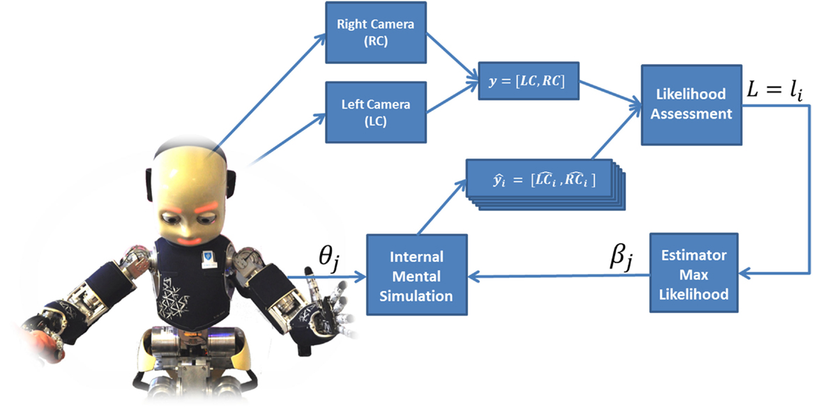
Figure 1. The iCub humanoid robot uses its internal mental simulation to imagine (generate synthetic images of) the hand pose in real time. By comparing the generated images $\left({\widehat{y}}_i\right)$ to the ones obtained through stereo vision (y), it simultaneously achieves better hand pose estimation and automatic calibration of the internal model.

We report experiments both in simulation, with the iCub dynamic simulator (Tikhanoff et al., 2008), and with the real iCub humanoid robot. The real-time implementation on the real robot is made possible by two techniques: GPU programing, to achieve faster computation, and an edge-based metric to compare the visual hypothesis with the actual visual perception. This is essential to improve robustness in real-world scenes, with a natural non-structured background.

Our solution draws inspiration from human development and learning, as: (i) the internal model is updated online based on the visual feedback of the hand, as infants seem to do between 4 and 8 months of age and (ii) the estimation of the pose of the end-effector results from the Bayesian integration of the sensory (visual) feedback and the predictions made by the internal model, a strategy that seems to characterize human perception as well, as described in Körding and Wolpert (2004).

The rest of the paper is organized as follows. In Section “Related Work,” we report the related work in robotics and we highlight our contribution more specifically. Then in Section “Proposed Method,” we formulate the problem and our proposed solution. We provide details on the body schema implementation, on the robotic platform used and on the error metrics employed (see Experimental Setup) and we present experimental results in simulation and with the real robot (see Results). Then, in Section “Discussion,” we discuss the proposed method and the results achieved. Finally, in Section “Conclusion and Future Work,” we draw our conclusions and sketch the future work.

2. Related Work

Reaching for objects and manipulating them is a crucial behavior in both humans and robots. While the classical approach in robotics is to rely on analytical models for motion control, humans learn such models from motor experience.

A number of works have proposed computational models to acquire these abilities through learning, without relying on any explicit model (Reinhart and Steil, 2009; Ciancio et al., 2011; Caligiore et al., 2014; Peniak and Cangelosi, 2014).

An alternative approach is to learn a model from sensorimotor data, and use the model for control. Such a model is typically referred to as “body schema.”

The acquisition and adaptation of a robot body schema has been a topic of considerable attention [see, for example, Hoffmann et al. (2010) for a review up to the year 2010]. Learning (or adapting) the body schema of a humanoid robot can be seen also as a calibration problem, in which the goal is to align the reference frame located in the eyes, where visual information about the environment is obtained, with the one centered in the hand (i.e., eye-hand calibration). Clearly, in order to accurately perform reaching and grasping actions a good calibration of these reference frames is required.

Since the visual estimation of the hand pose is a very challenging task, a way to simplify the calibration problem is to use a marker to visually detect the end-effector (i.e., the robot hand, in the humanoid case). For instance, the method used by Birbach et al. (2012) requires 5 min of data acquisition during specific robot movements with a special marker in the robot wrist. It optimizes offline some parameters of the kinematic chain (angle offsets and elasticity) of an upper humanoid torso using non-linear least squares.

Online solutions have been studied, for example, in Ulbrich et al. (2009) and Jamone et al. (2012), in which visual markers are used to easily detect the hand position. The inclusion of additional parts into the kinematic chain (i.e., tools) has been considered as well in Jamone et al. (2013a,b).

In general, the adoption of a learning-by-doing strategy, in which a model is learned online during the execution of a goal-driven movement (goal-directed exploration (Jamone et al., 2011) or goal babbling (Rolf, 2013)), has been shown to improve learning performances, for example, by reducing the time required for convergence. Moreover, it allows to learn not only forward models but also inverse models, including, for example, the inverse kinematics of a redundant robot system (Rolf et al., 2010; Damas et al., 2013).

Although visual servoing techniques have been studied since the early 1980s (Agin, 1980) and a number of advanced solutions have been proposed during the last 30 years (Chaumette and Hutchinson, 2007), real-time reaching and grasping tasks in humanoid robots are often performed without any visual feedback of the hand (Saxena et al., 2008; Ciocarlie et al., 2010). Also according to Bohg et al. (2014), very few methods for grasping control take advantage of vision to correct the pose of the robot end-effector. The main reason for this is that the visual estimation of the pose of the end-effector is difficult to achieve and computationally expensive; therefore, such visual feedback is typically noisy and cannot be obtained at a fast rate. However, purely open-loop reaching and grasping can hardly be successful, because the robot models are typically not accurate enough. For example, in Figueiredo et al. (2012) grasping is performed in kitchenware objects using a very precise robotic arm; however, some of the grasping experiments failed due to “contact between the hand and the object before grasping.” These undesired and unexpected premature contacts can be mitigated with a visual servoing approach.

Chaumette and Hutchinson (2006) define visual servoing as a feedback closed-loop control strategy based on vision. Many visual servoing applications rely on eye-in-hand frameworks, where the cameras are attached to the robot end-effector (La Anh and Song, 2012; Ma et al., 2013). In humanoid robots, the cameras are placed in the head, and visual servoing can be done with an eye-to-hand approach (Hutchinson et al., 1996). Most applications of eye-to-hand visual servoing use markers in the end-effector in order to estimate its pose.

In Kulpate et al. (2005), the use of a single camera, a landmark in the hand (a light bulb emitting a red light) and a flat mirror, improves the estimation of the hand position and orientation. In Vahrenkamp et al. (2008), a red ball is attached to the robot wrist to allow for precise grasping using stereo calibrated vision. The humanoid REEM is used in Agravante et al. (2013) to perform reaching and grasping with visual feedback, using special markers on the hand and on the objects; the results show how the reaching motion planned on the basis of the robot kinematic model was not accurate enough to allow for precise object grasping, and how the inclusion of a visual servoing component could accommodate for such inaccuracies.

Marker-free solutions have been explored as well, either for body schema adaptation or for visual servoing control. The solution proposed in Ulbrich et al. (2012) is based on the decomposition of the kinematic chain into smaller segments; then, both offline and online learning solutions are proposed to learn the kinematic structure of the robot. Although it seems that no markers are used, no description is present about how the end-effector pose is measured. In Fanello et al. (2014), eye-hand calibration is realized by performing several ellipsoidal arm movements with a predefined hand posture, tracking the tip of the index finger in the camera images. Optimization techniques are employed to learn the transformation between the fingertip position obtained by the stereo vision and the one computed from the forward kinematics. Such transformation is then used to calibrate the kinematics. However, the hand orientation is not considered.

A marker-less visual servoing strategy can be used if one can estimate the pose of the robot hand using visual data. This is a challenging problem per se that has been studied both in Human-Computer Interaction and in Robotics (see Erol et al. (2007) for a review up to the year 2007). A few interesting works in robotics have used machine learning techniques to deal with the problem of robot hand detection. Leitner et al. (2013) used the Cartesian Genetic Programming method to learn how to detect the robot hand inside an image from visual examples. Online Multiple Instance Learning was used by Ciliberto et al. (2011) for the same task (detect the robot hand), through the use of proprioceptive information from the arm joints and visual optic flow to automatically label the training images. However, in both works the hand orientation is neglected – only the position of the hand is learned. The work by Gratal et al. (2011) proposes a 3D-model based approach and an edge based error function to estimate the pose of the Schunk Dexterous Hand. This method is similar to ours as they exploit also graphics acceleration techniques and an edge-based approach. However, their optimization method is based on Virtual Visual Servoing (Comport et al., 2006) that, being a gradient based method, is prone to converge to local minima. On the contrary, we propose a sequential Monte Carlo method that is robust to non-convex/non-gaussian error functions.

2.1. Our Contribution

This paper extends our previous work on eye-hand adaptation in a humanoid robot (Vicente et al., 2014) and its GPGPU implementation (Vicente et al., 2015), by (i) comparing the influence of the number of particles in the estimation of the pose of the end-effector; (ii) performing an edge-based likelihood on the real robotic platform, and (iii) exploiting the derived models for the closed-loop control of the robot end-effector using visual feedback.

Our proposed system outperforms the related works described above by combining a number of features that are, in our opinion, fundamental to obtain an accurate control of goal-directed movements in humanoid robots. Our method does not use any special marker in the robot end-effector or in the robot wrist – it is a marker-free system. We estimate the 6D end-effector pose, rather than only the position, and we perform this estimation online during reaching tasks – our method does not require the execution of specific movements to calibrate the body schema. Moreover, we exploit the body schema adaptation and the real-time estimation of the end-effector pose to perform a marker-free visual servoing control strategy that improves the accuracy of reaching movements. To the best of our knowledge, a system that combines these fundamental features and that is successfully implemented in a real humanoid robot was not yet proposed in the literature.

3. Proposed Method

The body schema adaptation can be seen as an internal process that occurs in the mind of the robot and on the perception of the self. We focus on the perception of the arms and hands by the visual system placed in the robot head. This problem is known in human sciences as eye-hand coordination. In robotics, the eye-hand coordination relies on computing the transformation between two reference frames: (i) the eye reference frame and (ii) the end-effector reference frame. In our case, the first is located in the center of the left-eye and the latter in the center of the hand palm (see Figure 2). Moreover, the end-effector pose is defined as the pose of the hand palm in the eye reference frame. In this work, we estimate the end-effector pose using vision (left and right images) and proprioception (encoder readings), and adapt the initial body schema to reduce the mismatches between the internal model prediction of the end-effector pose and the observed end-effector pose. According to the free-energy principle (Friston, 2010), biological agents try to minimize its free energy with the environment to achieve equilibrium. The free-energy principle tries to mathematically define how humans and animals optimize their expectation of the world. Thus, the free-energy measures the surprise present in perception given a generative model. The agent can suppress free energy by acting on the world (exciting the sensory input) or by changing its generative model to compensate the perception. Moreover, if we see the agent’s body schema as the hidden state of the generative model, one of the solutions to achieve the equilibrium is to perform the body schema adaptation, as proposed in this work.

FIGURE 2

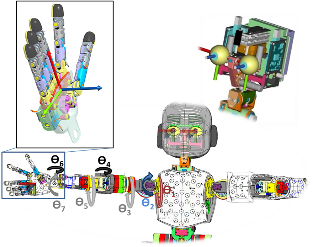
Figure 2. The end-effector’s pose (palm of the hand) is a function of the joints angles. Axis color notation: x-red; y-green; z-blue. (For a more detailed description visit: http://wiki.icub.org/wiki/ICubForwardKinematics). Best seen in color.

To achieve this goal, we consider two phases of reaching movements. First, an open-loop ballistic movement drives the end-effector to the vicinity of the target without visual feedback. During this period, vision is used to estimate the end-effector pose and adapt the internal model but the arm controller does not use this information. Second, a closed-loop control based on vision drives the robot’s end-effector to the desired final pose, relative to the target of interest. During this stage, the internal model continues its adaptation based on vision and the arm controller used the adapted model to move the arm. In this section, we describe our methodology to address these phases. We begin by introducing the body schema model of our humanoid robot. Then, we explain the end-effector’s vision based pose estimation method during the ballistic movement. Finally, we describe how to perform the control of the arm using the visual feedback.

3.1. Body Schema Modeling

Let us consider the problem of estimating the robot’s end-effector pose in the left camera’s reference frame (an analogous analysis can be done for the right camera). The real pose (x^r) can be represented by a generic 4 × 4 roto-translation matrix T. Using the robot kinematics function from the left camera to the hand palm 𝒦(⋅) and the vector of joint encoder readings θ (see Figure 2), an estimate of the pose can be obtained by:

${\widehat{\mathbf{T}}}_{\text{kin}}=\text{𝒦}\left(\mathrm{\theta }\right)$ (1)

However, several sources of error may affect this estimate. Let us consider the existence of calibration errors (bias). This source of error can be encoded in many different ways. We propose to encode it in the robot’s joint space, i.e.,

${\mathrm{\theta }}^r=\mathrm{\theta }+\mathrm{\beta }$ (2)

where θ^r are the real angles; θ are the measured angles; β are joint offsets representing calibration errors. Given an estimate of the joint offsets $\widehat{\mathit{\beta }}$, a better end-effector’s pose estimate can be computed by:

${\widehat{\mathbf{T}}}_{\text{joint}}=\text{𝒦}\left(\mathrm{\theta }+\widehat{\mathit{\beta }}\right).$ (3)

Another solution is to encode the calibration error in Cartesian space using a roto-translation matrix defined as:

${\widehat{\mathbf{T}}}_{\text{Cart}}=\text{𝒦}\left(\mathrm{\theta }\right)\cdot {\widehat{\mathbf{T}}}_{\text{ERR}}$ (4)

where T_ERR encodes the calibration errors.

The generalization of the learned parameters to other parts of the workspace was analyzed before in Vicente et al. (2015). We have shown that a parameterization of the error in the body schema in terms of joint offsets generalizes better to other parts of the workspace when compared to the non-calibrated case and to the Cartesian Error modeling, because the dominant sources of error are actually joint offsets.

Therefore, in this work, the learning process of the internal model consists in estimating the joint’s offsets (β) in the kinematic chain [see equation (2)]. Moreover, as we have access to the proprioceptive feedback (θ), estimating the joint offsets rather than the absolute joint values is a more effective approach: (i) the search space is smaller and (ii) we can use the adapted body schema (learned offsets) in other movements without re-learning it from scratch.

3.2. State Estimation with Sequential Monte Carlo Methods

Let x be a generic state vector and y the observation vector. Assuming that y depends stochastically on x at time t¹ one can devise a Bayesian filter to estimate the state x from the observation y. The Bayesian filter consists of two steps: prediction and update. In the former, we calculate x_t from the previous state x_t–1 according to the following equation:

$p\left({\mathbf{x}}_t|{\mathbf{y}}_{1:t-1}\right)=\int p\left({\mathbf{x}}_t|{\mathbf{x}}_{t-1}\right)\cdot p\left({\mathbf{x}}_{t-1}|{\mathbf{y}}_{1:t-1}\right)d{\mathbf{x}}_{t-1}$ (5)

where p(x_t|x_t–1) is the transition probability and p(x_t–1|y_1:t−1) the previous estimation of the state at time t − 1. In the second step, we update the posterior distribution with the last observation:

$p\left({\mathbf{x}}_t|{\mathbf{y}}_{1:t}\right)=\mathrm{\eta }\cdot p\left({\mathbf{y}}_t|{\mathbf{x}}_t\right)\cdot p\left({\mathbf{x}}_t|{\mathbf{y}}_{1:t-1}\right)$ (6)

where η is a normalization factor and the probability p(y_t|x_t) is called measurement probability.

The particle filter, also known as sequential Monte Carlo (SMC) method, is a non-parametric implementation of the Bayes filter, where we approximate the posterior distribution equation (6) by a finite number of samples, called particles:

$p\left({\mathbf{x}}_t|{\mathbf{y}}_{1:t}\right)\approx {\displaystyle \sum _{m=1}^M}{\mathrm{\omega }}^{\left[m\right]}\mathrm{\delta }\left({\mathbf{x}}_t-{\mathbf{x}}_t^{\left[m\right]}\right)\cdot {\left({\displaystyle \sum _{m=1}^M}{\mathrm{\omega }}^{\left[m\right]}\right)}^{-1}$ (7)

where M is the number of particles, ${\mathbf{x}}_t^{\left[m\right]})$ (with 1 < m < M) is one particle, ω^[m] is the weight of particle m and ${\displaystyle \sum _{m=1}^M}{\mathrm{\omega }}^{\left[m\right]}=1$. The three stages of the particle filter are as follows:

1. Prediction: we sample ${\mathbf{x}}_t^{\left[m\right]}$ from $p\left({\mathbf{x}}_t|{\mathbf{x}}_{t-1}^{\left[m\right]}\right)$ adding these particles to a temporary set ${\overline{\sout{𝒳}}}_t$.

2. Update: we receive a new observation vector, y_t, and update the particle weight or particle likelihood (ω^[m]) according to: ${\mathrm{\omega }}^{\left[m\right]}=p\left({\mathbf{y}}_t|{\mathbf{x}}_t^{\left[m\right]}\right)$.

3. Re-sampling: the particles are sampled according to their weight: ω^[m]. This step is of paramount importance for the particle filter algorithm to work properly, Thrun et al. (2005) called it: the “trick” of the algorithm. We replace the M particles in the temporary set ${\overline{\sout{𝒳}}}_t$ by another M particles according to their weights ω^[m]. Whereas in the temporary ${\overline{\sout{𝒳}}}_t$ the particles were distributed according to equation (5), after this step they are distributed (approximately) according to the posterior [see equation (6)].

For further details on Bayes and Particle filters, one can read Thrun et al. (2005).

3.3. Parameter Estimation with Sequential Monte Carlo Methods

In spite of being often used to track dynamic states, some modifications to the sequential Monte Carlo (SMC) methods have been proposed to estimate static parameters as well. In Kantas et al. (2009), the authors perform an overview of SMC methods for parameter estimation. Let, again, x be the initial non-static state vector and β the static parameter vector. An augmented state is defined as follows:

${\mathbf{x}}^{\text{aug}}={\left[\mathbf{x}\mathrm{\beta }\right]}^T$ (8)

One of the proposed solutions to estimate the parameters β is to introduce an artificial dynamics, changing from a static transition model:

${\mathrm{\beta }}_t={\mathrm{\beta }}_{t-1}$ (9)

to a slowly time-varying one:

${\mathrm{\beta }}_t={\mathrm{\beta }}_{t-1}+\mathbf{w}$ (10)

where w is an artificial dynamic noise that decreases when t increases.

3.3.1. Our Formulation

In our particular case, we are interested in the estimation of the end-effector pose (x) as well as the calibration error parameters β. We define the augmented state vector at time t as:

${\text{X}}_t^{\text{aug}}={[\text{vec(𝒦}\left({\mathrm{\theta }}_{\text{t}}+{\mathrm{\beta }}_t\right)\text{)}{\mathrm{\beta }}_t]}^{\text{T}}$ (11)

where 𝒦(⋅) is the robots kinematics function [see equation (3)] and the vector β is composed of the offsets in the kinematics chain from the camera to the end-effector. To reduce the complexity of the problem, we only consider the angular offsets of the arm kinematic chain (7 DOF), as the head chain is assumed to be calibrated, for instance, using the procedure defined in Moutinho et al. (2012). Also miscalibration in the finger joints has a smaller impact in the observations since they are at the end of the kinematic chain.

The offsets in equation (11) define the parameter vector, β = [β₁β₂β₃β₄β₅β₆β₇]^T, as an unobserved Markov process where β_i is the offset in joint i of the arm assuming an initial distribution:

$p\left({\mathrm{\beta }}_0\right)$ (12)

According to the general model in equation (10), β is the vector composed by the offsets in the arm, and the artificial noise w ~ 𝒩(0, K) is a zero mean Gaussian noise with a given diagonal covariance $\mathbf{K}={\mathrm{\sigma }}_s^2{\mathbf{I}}_7$ and σ_s is an appropriately defined SD reflecting the magnitude of the calibration errors.

The first part of the augmented state, 𝒦(θ_t + β_t), is deterministic given β_t since it is based on the robot kinematics function and the noiseless encoder readings, thus estimating the posterior distribution of the full state is equivalent to posterior distribution of the particles:

$p\left({\mathrm{\beta }}_t|{\mathbf{y}}_{1:t},{\mathrm{\theta }}_{1:t}\right)\equiv p\left({\mathbf{x}}_t^{\text{aug}}|{\mathbf{y}}_{1:t}\right)$ (13)

We use a SMC method to approximate the posterior distribution defined in equation (13) by a set of random samples (particles):

${\mathbf{B}}_t:=\left\{{\mathrm{\beta }}_t^{\left[1\right]},{\mathrm{\beta }}_t^{\left[2\right]},{\mathrm{\beta }}_t^{\left[3\right]},...,{\mathrm{\beta }}_t^{\left[M\right]}\right\}$ (14)

where M is the number of particles, ${\mathrm{\beta }}_t^{\left[m\right]}$ (with 1 < m < M) is one state sample, and B_t is the particle set at time t. The a posteriori density distribution is approximated by the weighted set of particles:

$p\left({\mathrm{\beta }}_t|{\mathbf{y}}_{1:t},{\mathrm{\theta }}_{1:t}\right)\approx {\displaystyle \sum _{m=1}^M}{\mathrm{\omega }}^{\left[m\right]}\mathrm{\delta }\left({\mathrm{\beta }}_t-{\mathrm{\beta }}_t^{\left[m\right]}\right)\cdot {\left({\displaystyle \sum _{m=1}^M}{\mathrm{\omega }}^{\left[m\right]}\right)}^{-1}$ (15)

where ω^[m] is the weight of particle m, δ(.) is the Dirac delta function, and the last factor is the normalization factor. In the beginning of each time step t, all the particles have the same weight: ${\mathrm{\omega }}^{\left[m\right]}=\frac{1}{M}$. Under the Markov assumption, we can compute recursively p(β_t|y_1:t, θ_1:t) sampling from the previous estimation p(β_t–1|y_1:t–1, θ_1:t–1).

The filter has three stages as defined in Section “State estimation with Sequential Monte Carlo Methods”: prediction, update, and re-sampling:

1. Prediction: we sample ${\mathrm{\beta }}_t^{\left[m\right]}$ from $p\left({\mathrm{\beta }}_t|{\mathrm{\beta }}_{t-1}^{\left[m\right]}\right)$, according to the transition [see equation (10)], in our case ${\mathrm{\beta }}_t^{\left[m\right]}={\mathrm{\beta }}_{t-1}^{\left[m\right]}+\mathbf{w}$.

2. Update: we receive a new observation vector, y_t, and update the particle weight (ω^[m]) according to: ${\mathrm{\omega }}^{\left[m\right]}=p\left({\mathbf{y}}_{\text{t}}|{\mathrm{\beta }}_t^{\left[m\right]}\right)$, i.e., the particle likelihood. Our observation model and the particle likelihood are defined in Section “Observation Model.”

3. Re-sampling: the particles are sampled according to their weight using the systematic re-sampling method (Hol et al., 2006), which guarantees that a particle with a weight greater than 1/M is always re-sampled, where M is the total number of particles.

3.4. Observation Model

In this section, we address the problem of how to calculate the measurement probability in equation (6). The measurement probability can also be seen as the particle weight/likelihood after normalization. Our humanoid robot has two sources of information: (i) cameras on the eyes (visual sensing) and (ii) head and arm encoders (proprioceptive sensing). These two sources of information are related by the following model:

${\mathbf{y}}_t=\mathbb{ℱ}\left({\mathrm{\theta }}_t+{\mathrm{\beta }}_t\right)+\mathrm{\eta }$ (16)

where θ_t are the encoder readings and β_t the actual offsets in the joints at time step t. The function ℱ(.) encodes the kinematic structure [see equation (1)], appearance of the robot, the camera’s intrinsic parameters, and the image rendering model provided by a computer graphics engine able to generate realistic views of the robot. The actual observation, y_t, is a random variable that concatenates the images acquired from the left and right cameras and η an image random noise (due to diverse non-modeled sources, e.g., specularities, shadows, camera jitter, etc., not necessarily Gaussian).

To sample from this model, we use the computer graphics rendering engine that generates virtual images of the robots cameras for arbitrary values of the vector β and encoder readings θ (see Figure 3):

${\widehat{\mathbf{y}}}_t^{\left[m\right]}=\text{ℱ}\left({\mathrm{\theta }}_t+{\mathrm{\beta }}_t^{\left[m\right]}\right)$ (17)

where ${\widehat{\mathbf{y}}}_t^{\left[m\right]}$ represents the concatenation of the virtual images in the left and right cameras of the robot simulator for each generated hypothesis (particle). The particles can be seen as the multiple hypotheses generated by the brain while imagining the possible images consistent with the current state.

FIGURE 3

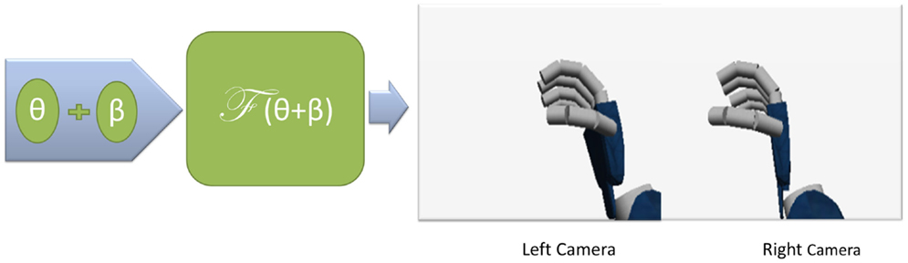
Figure 3. Image generation in the internal mental simulator. The observation is defined as the concatenation of the left and right cameras.

From the comparison between the real measurements y_t and the virtual measurements ${\widehat{\mathbf{y}}}_t^{\left[m\right]}$, through a suitable function $g\left({\mathbf{y}}_t,{\widehat{\mathbf{y}}}_t^{\left[m\right]}\right)$, we can compute the likelihood of β at time t:

$l\left({\mathrm{\beta }}_t^{\left[m\right]}\right)=p\left({\mathbf{y}}_t|{\mathrm{\theta }}_t,{\mathrm{\beta }}_t^{\left[m\right]}\right)\propto g\left({\mathbf{y}}_t,{\widehat{\mathbf{y}}}_t^{\left[m\right]}\right)$ (18)

We have defined two different approaches for implementing the comparison function g(⋅,⋅). One is based on the hand’s silhouette through image segmentation and the other is based on image contours through edge extraction.

3.4.1. Silhouette Segmentation

In this approach, we use the segmented binary images from the real and virtual cameras (see Figure 4). To compute the similarity between the real and virtual binary masks (silhouettes), we use the Jaccard coefficients (s_Jc) (see Cox and Cox (2000) for more detail). Let R(y) be the real silhouette and R($\widehat{\mathbf{y}}$) the virtual silhouette. The Jaccard coefficient is defined as follows:

$s_{\mathit{Jc}}\left(\mathbf{y},\widehat{\mathbf{y}}\right)=\frac{\#\left(\mathbf{R}\left(\mathbf{y}\right)\cap \mathbf{R}\left(\widehat{\mathbf{y}}\right)\right)}{\#\left(\mathbf{R}\left(\mathbf{y}\right)\cup \mathbf{R}\left(\widehat{\mathbf{y}}\right)\right)}$ (19)

where # denotes the number of pixels in the region.

FIGURE 4

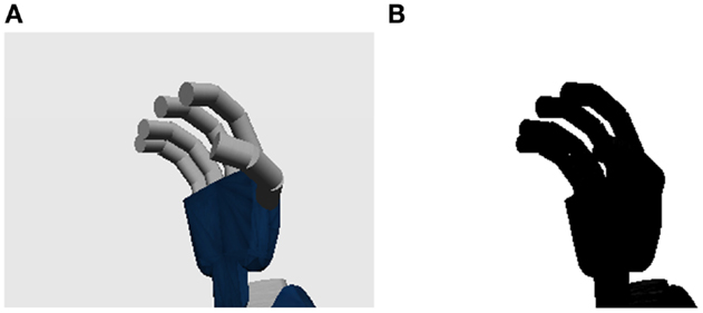
Figure 4. Example of silhouette segmentation. The silhouette is a binary image (B) extracted from an image of the iCub hand (A) computed by image segmentation techniques. Results obtained from the iCub simulator.

The numerator term in equation (19) is measuring how similar and overlaid are the two silhouette regions and the denominator is normalizing the metric to a range [0,1]. Therefore, we define the likelihood model as follows:

$p\left({\mathbf{y}}_t|{\mathrm{\beta }}_t,{\mathrm{\theta }}_t\right)\propto s_{\text{Jc}}\left({\mathbf{y}}_t,{\widehat{\mathbf{y}}}_t\right)$ (20)

In order to apply this approach, we need a good segmentation of the area of interest in the image. In this work, this is a feasible approach if one of the following conditions are met: either the head of the robot is static and a silhouette can be extracted by background segmentation methods, or the background is uniformly colored and a good silhouette can be obtained by color segmentation methods. In case, the head is moving or the background is cluttered, this approach is not robust and the edge-based method, described in the following section, is preferred.

3.4.2. Edge Extraction Approach

In this approach, the segmentation of the area of interest is not needed, instead, we exploit the edge information extracted from images, which is more robust to clutter, thus, more suitable to realistic environments. For this approach, we compute the average distance between the edges of the real image to the closest edge in the virtual image, and denote this quantity $\overline{d}$. A perfect match between the real and virtual images will correspond to $\overline{d}=0$ whereas bad matches will correspond to large values of $\overline{d}$. The likelihood function is thus defined as:

$p\left({\mathbf{y}}_t|{\mathrm{\beta }}_t,{\mathrm{\theta }}_t\right)\propto {\exp }^{-{\mathrm{\lambda }}_{\text{edge}}\cdot \overline{d}}$ (21)

where λ_edge is a tuning parameter to control sensitivity in the distance metric.

To compute $\overline{d}$, we make use of the distance transform (Borgefors, 1986). The distance transform (DT) consists in the application of an edge detector to the image (e.g., Canny (1986)) and then, for each pixel, compute its distance to the closest edge point. This distance has a minimum of 0 pixel and a maximum of 255 pixel, since the DT result is a 8-bit single-channel image. In Figure 5, we give an example of the right camera’s image and the corresponding edge and distance transform images.

FIGURE 5

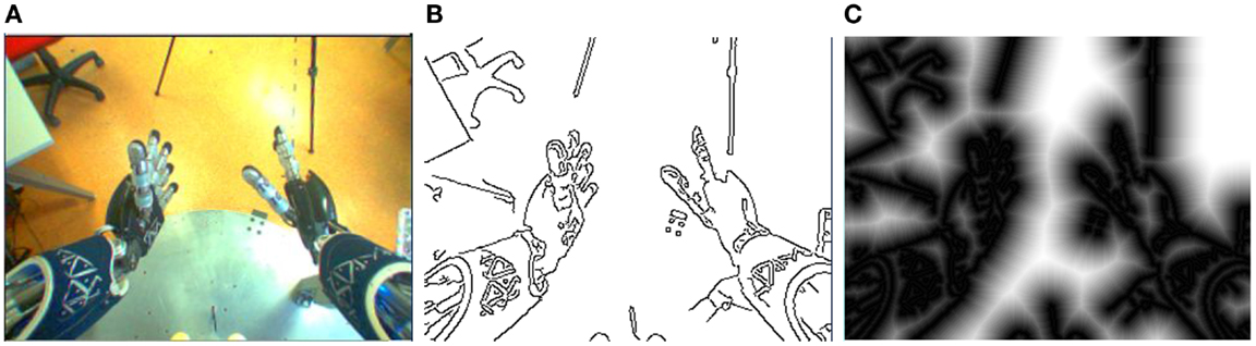
Figure 5. Example of the computation of the edges and distance transform of the iCub hand in a real environment on the right camera. (A similar example can be shown for the left camera.) (A) is the input image, (B) shows the edges extraction using Canny, 1986, and (C) the distance transform using Borgefors, 1986.

Let D(y) be the distance transform of the real images and E($\widehat{\mathbf{y}}$^[m]) be the edge map of the virtual images (binary image indicating the edge pixels).

The average distance, ${\overline{d}}^{\left[m\right]}$ for each particle, can be efficiently computed using the Chamfer matching distance (Borgefors, 1988) defined as follows:

${\overline{d}}^{\left[m\right]}=\frac{1}{k}\cdot {\displaystyle \sum _{i=0}^N}\mathbf{E}\left({\widehat{\mathbf{y}}}^{\left[m\right]}\left(i\right)\right)\cdot \mathbf{D}\left(\mathbf{y}\left(i\right)\right)$ (22)

where k is the number of edge pixels in the virtual image, i is an index that runs over all pixels, and N is the total number of pixels.

3.5. Computing the Parameter Estimate

Although the parameters are represented at each time step as a distribution approximated by the particles, for practical purposes we must compute our best guess of the parameter vector $\widehat{\mathit{\beta }}$. We use a kernel density estimation (KDE) to smooth the weight of the particles according to the information of neighbor particles, and choose the particle with the highest smoothed weight (ω′^[i]) as our parameter estimate:

${\mathrm{\omega }\prime }^{\left[i\right]}={\mathrm{\omega }}^{\left[i\right]}+\mathrm{\alpha }\cdot \frac{1}{M}{\displaystyle \sum _{m=0}^M}{\mathrm{\omega }}^{\left[m\right]}\cdot K\left({\mathrm{\beta }}^{\left[i\right]},{\mathrm{\beta }}^{\left[m\right]}\right)$ (23)

where ω^[i] is the particle likelihood, α is a smoothing parameter, M is the number of particles used in our SMC implementation, and β^[i] is the particle we are smoothing. The sum term is the influence of the neighbors in the score of particle i. K is a kernel specifying the influence of one particle in others based on their distance. We use a Gaussian Kernel in our experiments:

$K\left({\mathrm{\beta }}^{\left[i\right]},{\mathrm{\beta }}^{\left[j\right]}\right)=\frac{1}{\sqrt{\mathrm{2\pi }|\Sigma |}}{e}^{\left[-\frac{1}{2}{\left({\mathrm{\beta }}^{\left[i\right]}-{\mathrm{\beta }}^{\left[j\right]}\right)}^T{\Sigma }^{-1}\left({\mathrm{\beta }}^{\left[i\right]}-{\mathrm{\beta }}^{\left[j\right]}\right)\right]}$ (24)

where Σ is the co-variance matrix and |Σ| its determinant.

Since the joints’ offsets (β) are independent of each other, Σ will be a diagonal matrix:

$\Sigma ={\mathrm{\sigma }}_{\text{KDE}}^2\cdot I_7$ (25)

where σ_KDE is the SD in each joint, which we assume equal. This parameter determines if two particles are close or not. If we have a high σ_KDE, all particles will be “close” to each other. On the other hand, if we have a small σ_KDE, all particles will be fairly isolated in the world resulting in ω′^[i] ≈ ω^[i].

It is worth to note that due to the redundancy in the robot kinematics (joints space is 7DOF while the end-effector pose is 6DOF) different solutions in the set B_t may correspond to the same target pose. Therefore, the likelihood function l(β) is multimodal and a particular choice of $\widehat{\mathit{\beta }}$ will be just one set of offsets that can explain the end-effector’s appearance in the images. For this reason, the proposed method with sequential Monte Carlo, which does not assume any particular distribution of the posterior, is a suitable parameter estimation approach.

3.6. Controlling the End-Effector

In this work, we focus on the control of the arm to obtain a desired end-effector’s pose using the robot internal body schema. We have implemented two control modalities: (i) an open-loop “ballistic” movement and (ii) a closed-loop strategy exploiting visual feedback.

3.6.1. Open-Loop

The open-loop control is the dominant control mode in robotics manipulation. It relies on accurate calibration of the robot system and accurate object sensing. It exploits the inverse kinematics of the head-arm-hand chain, from the eye to the end-effector and only uses visual sensing for the initial estimation of the object/target pose. During arm control, only proprioceptive feedback is used. The open-loop control relies on solving the robot’s inverse kinematics (𝒦⁻¹):

${\mathbf{q}}^{\text{d}}={\text{𝒦}}^{-1}\left({\mathbf{x}}^{\text{d}}\right)$ (26)

where q^d is the joints configuration (command) that leads to the desired end-effector’s pose (x^d) and 𝒦⁻¹ the inverse kinematics function.

The trajectory between the initial joints configuration (qⁱ) and the desired one (q^d) is a linear trajectory in the joint space, performing a movement with a constant velocity according to the following equation:

${\mathbf{q}}_{t+1}={\mathbf{q}}_t+\frac{{\mathbf{q}}^d-{\mathbf{q}}^i}{\mathrm{\Delta }t}$ (27)

where q_t is the joint command at time t and Δt is the desired movement duration.

3.6.2. Closed-Loop

In the closed-loop approach, instead of controlling the position of the joints, we control the joint velocities $\dot{\mathbf{q}}$ based on visual feedback.

As mentioned in Section “Related Work,” our problem is an instance of eye-to-hand visual servoing. Two control modalities are common in visual servoing approaches: (i) image-based control, where the arm’s motion is determined by the error between the current and desired configurations in the image coordinates or (ii) a position-based approach, where the arm’s motion is determined by the error between the current and desired 6D poses of the end-effector. Our approach is a position-based strategy in an eye-to-hand configuration. See Hutchinson et al. (1996) for a more detailed taxonomy of visual servoing strategies.

Following the notation in Siciliano and Khatib (2007), the error (e) to be minimized is defined as follows:

$\mathbf{e}={\mathbf{x}}^{\text{c}}-{\mathbf{x}}^{\text{d}}$ (28)

where x^d is the desired 6D pose of the end-effector and x^c the current.

The relationship between the joint velocities and the time variation of the 6D pose error is given by:

$\dot{\mathbf{e}}=\mathbf{J}\left(\mathbf{q}\right)\cdot \dot{\mathbf{q}}$ (29)

where J(q) is the robot Jacobian from the left-eye to the end-effector reference frame.

If we defined $\dot{\mathbf{e}}=-\mathrm{\lambda }\cdot \mathbf{e}$ (to ensure an exponential decoupled decreasing error) and invert the robot Jacobian (J(q)) by using the Moore-Penrose pseudo inverse, we end up with the following control law:

$\dot{\mathbf{q}}=-\mathrm{\lambda }\cdot {\mathbf{J}}^{†}\left(\mathbf{q}\right)\cdot \mathbf{e}$ (30)

where J^†(q) is the pseudo-inverse in the joint angles q.

In our case, as we correct the joint angles on the robot arm, the control law with the improved robot Jacobian will be:

$\dot{\mathbf{q}}=-\mathrm{\lambda }\cdot {\mathbf{J}}^{†}\left(\mathrm{\theta }+\widehat{\mathit{\beta }}\right)\cdot \mathbf{e}$ (31)

where θ are the encoder readings and $\widehat{\mathit{\beta }}$ the joint offset vector.

4. Experimental Setup

4.1. Robotic Platform

The iCub (see Figure 1) is a humanoid robot for research in artificial intelligence and cognition. It has 53 motors that move the legs, waist, head, arms, and hands, and it has the average size of a 3-year-old child. It was developed in the context of the EU project RobotCub (2004–2010) and subsequently adopted by more than 25 laboratories worldwide. Its stereo vision system (cameras in the eyeballs), proprioception (motor encoders), touch (tactile fingertips and artificial skin), and vestibular sensing (IMU on top of the head) are important characteristics that allow the study of autonomy in humanoid robots. The robot is equipped with a dynamic simulator (Tikhanoff et al., 2008) that can be controlled using the same software that is used for the real robot. We resort to this simulator in a number of experiments in order to evaluate the performance of our approach with precise ground-truth (that we cannot access on the real robot).

4.2. Body Schema

The body schema can be considered the agent’s knowledge about the kinematics, posture, and appearance of its body parts. The body schema is a mental state that includes sensory information about the self and the world and about the relationships between the body parts. In this work, we have implemented the iCub’s body schema on 3D computer graphics engines. Graphics engines permit an effective generation of mental images of body states through the knowledge of the kinematic structure of the robot, and its body appearance. The internal mental simulator projects the 3D simulated body into the robot vision. In particular, we are interested in the projection of the arms and hands – the end-effectors. The capabilities of the internal mental simulator are similar to the real agent: (i) we can control the end-effector to a given pose, (ii) it has proprioceptive sensing, thus, we can acquire the current joint values of the arm and head, and (iii) it has stereo vision – projecting the 3D world into 2D images.

4.3. Error Metrics

4.3.1. Position and Orientation

In order to evaluate the accuracy of our method, we compute the Cartesian error (E_Cartesian) composed of position and orientation errors between two generic poses, A and B, as:

$E_{\text{Cartesian}}=\left[d_o,d_p\right]$ (32)

The general orientation error (d_o) is defined as:

$d_o\left({\mathbf{R}}_A,{\mathbf{R}}_B\right)=\sqrt{\frac{\left|\right|\text{logm}\left({\mathbf{R}}_A^T{\mathbf{R}}_B\right)|{|}_F^2}{2}}\frac{180}{\mathrm{\pi }}{[}^{\circ }]$ (33)

where R_A and R_B are two rotation matrices from the eye reference frame to the end-effector frame. The principal matrix logarithm, logm, with the Frobenius norm, (||⋅||_F), implements the usual distance on the group of rotations. The general position error between the two different poses is computed by the Euclidean distance, dp(P_A, P_B):

$d_p\left({\mathbf{P}}_A,{\mathbf{P}}_B\right)=\sqrt{{\left(x_A-x_B\right)}^2+{\left(y_A-y_B\right)}^2+{\left(z_A-z_B\right)}^2}$ (34)

where P_A and P_B are 3D Cartesian positions of the end-effector.

4.3.2. Defined Poses

In this work, we define four different poses. The real pose (x^r) is defined as:

${\mathbf{x}}^r=\left[{\mathbf{P}}^r\text{vec}\left({\mathbf{R}}^r\right)\right]$ (35)

where R^r is the real rotation matrix and P^r the real 3D position. This pose is the ground-truth data for evaluating the method. In the simulation experiments, this is the pose with the introduced artificial offsets. The second pose is the desired pose (x^d) which is the pose that we want to achieve during the reaching task:

${\mathbf{x}}^d=\left[{\mathbf{P}}^d\text{vec}\left({\mathbf{R}}^d\right)\right]$ (36)

The initial pose (xⁱ) is the initial joint configuration at the beginning of the reaching movement. Finally, the estimated pose (x^e) that is the robot’s forward kinematics applied to the sum of the measured joint angles θ (the proprioception) and the estimated β (or β = 0 when the adaptation is not performed):

${\mathbf{x}}^e=\left[{\mathbf{P}}^e\text{vec}\left({\mathbf{R}}^e\right)\right]$ (37)

4.3.3. Estimation and Reaching errors

The estimation error – E_estimation – is the difference between the real pose (x^r) and the estimated pose (x^e) using equations (33) and (34):

$E_{\text{estimation}}=\left[d_o\left({\mathbf{R}}^r,{\mathbf{R}}^e\right),d_p\left({\mathbf{P}}^r,{\mathbf{P}}^e\right)\right]$ (38)

The real reaching error – $E_{\text{reaching}}^r$ – is defined as the difference between the desired (x^d) and real pose (x^r):

$E_{\text{reaching}}^r=\left[d_o\left({\mathbf{R}}^d,{\mathbf{R}}^r\right),d_p\left({\mathbf{P}}^d,{\mathbf{P}}^r\right)\right]$ (39)

It measures how far the end-effector is from the target pose.

The estimated reaching error – $E_{\text{reaching}}^e$ – is defined as the difference between the desired (x^d) and estimated pose (x^e):

$E_{\text{reaching}}^e=\left[d_o\left({\mathbf{R}}^d,{\mathbf{R}}^e\right),d_p\left({\mathbf{P}}^d,{\mathbf{P}}^e\right)\right].$ (40)

It represents the robot’s belief on how far its end-effector is from the target pose.

4.4. Computer Specifications

The experiments were performed in a computer equipped with an Intel^® Xeon^® Processor W3503 at 2.4 GHz with two cores, two threads, and a 4-MB memory cache and a NVidia GeForce GTX 750 with 512 CUDA Cores, a base clock of 1020 MHz and 2048 MB of memory (RAM).

4.5. Experimental Settings

In this section, we describe the experimental parameters, common to all the presented results. We initialize the SMC with M = 200 particles, defining p(β₀) ~ 𝒩(0, Q) [see equation (12)] with a given diagonal covariance $\mathbf{Q}={\sigma }_i^2{\mathbf{I}}_7$ and σ_t = 5°. In all the experiments we started from scratch, i.e., the best estimation at t = 0 is the proprioception of the robot (β = 0). The artificial dynamic noise is initialized with σ_s = 4° and it decreases with t by a factor of 0.8:

${\mathrm{\sigma }}_s\left(t\right)={\mathrm{\sigma }}_s\left(t-1\right)\ast 0.8$ (41)

where t is the frame index. This value has a lower bound of 0.08° to allow continuous adaptation.

The kernel density estimation was initialized using a SD of σ_KDE = 1° in equation (23) and a neighborhood influence of α = 500 in equation (25).

5. Results

In this section, we report the experimental results. We divide them into two parts: simulations (Section “Simulation Results”) and real-world evaluations (Section “Real Robot Results”). In the former, we evaluate quantitatively our method comparing the body schema adaptation with the ground-truth measurements and in the latter we test our approach qualitatively in the real robot.

In Section “Reaching Movement and Body Schema Adaptation,” we show how the online adaptation of the body schema and the estimation of the pose of the end-effector allow to accurately reach for a desired pose, using a combined open-loop and closed-loop control scheme: (i) during the open-loop control (described in Section “Open-Loop”), the online body schema adaptation is performed, allowing for better estimation of the end-effector pose and (ii) during the closed-loop control (described in Section “Closed-Loop”), the end-effector pose feedback is exploited to accurately reach for the desired pose.

Then, in Section “Trade-Off between the Number of Particles and Estimation Accuracy,” we assess the performance of the internal model estimation procedure, evaluating the relationship between the number of particles used in the optimization procedure and the accuracy of the estimation.

Finally, in Section “Real Robot Results,” we show the method working in the real world: the iCub robot performs online adaptation of its body schema (i.e., including both arms) and real-time estimation of the pose of its end-effectors (i.e., both right and left hands) exploiting visual feedback from its cameras, in an unstructured environment (i.e., with natural background in the images).

5.1. Simulation Results

In the simulation experiments, we use the iCub simulator both as robot and as internal mental simulation. The iCub simulator is a realistic software that uses ODE (Open Dynamic Engine) for simulating the motion of rigid bodies and their physical interaction. It uses the same software and control architecture of the real iCub robot. In order to consider the iCub simulator a realistic model of the real robot, we introduce artificial angular offsets in the 7 DOFs of the right arm kinematic chain. We define ETA = [5, 4, 3, −2, 3, −7, 3]; these offsets have the same order of magnitude of the calibration errors, we typically encounter on the real robot. We use the same set of offsets in all the simulation experiments, in order to be able to compare the different results. Therefore, in these experiments the only difference between the robot and the internal mental simulation is the set of artificial offset; the goal of the body schema online adaptation is to compensate for these offsets.

Hand visual perception relies on the silhouette segmentation approach (described in Section “Silhouette Segmentation”); a homogeneous white background is located in front of the robot and the segmentation is performed based on color information. In general, the silhouette approach is effective in cases where the segmentation is easy (e.g., with the white background). In Section “Real Robot Results,” we will motivate the use of a different strategy, the edge-based approach (described in Section “Edge Extraction Approach”), for the real robot experiments, where we deal with natural background; such strategy could not, however, be used in these simulation experiments, because the texture model of iCub simulator is poor (based on simple cylinders and cubes of a homogeneous gray color) and too few edges are present in the images.

5.1.1. Reaching Movement and Body Schema Adaptation

In this first set of experiments, we have two main objectives: (i) evaluate the error in the end-effector pose estimation equation (38) during the movements, and (ii) show the convergence of the reaching error (real and estimated, equations (39) and (40), respectively) during the closed-loop control made possible by the body schema adaptation.

We define a constant duration of the open-loop phase (120 frames) in order to estimate a stable solution for the joint offsets (β) and we define 50 frames in the close-loop as the maximum number of frames to acquire during the reaching to the desired pose x^d using visual feedback. The error decaying factor presented in the closed-loop control section was initialized with the value λ = 5 [see equation (31)].

Overall, we perform 120 movements with different initial and final poses in order cover different areas of the working space: 4 different final poses with 10 initial poses, with 3 repetition of each movement. The results in this section show the mean and SD over the 120 experiments performed. We initialize our sequential Monte Carlo implementation with 200 particles and with β = 0, i.e., we always start the movements with the nominal non-calibrated model.

In Figure 6, we can see the mean and the SD of the end-effector pose estimation error during the movements. We show the error both with the nominal non-calibrated model (without online adaptation) and with the online adaptation. The algorithm converges to a good estimation after about 60 frames, improving it during the last part of the movement. It can be noticed that, in spite of having constant artificial offsets in the joints (i.e., a constant source of error), the pose estimation error in the non-calibrated case (without online adaptation, red dotted line in Figure 6) is not constant and it depends on the current arm configuration.

FIGURE 6

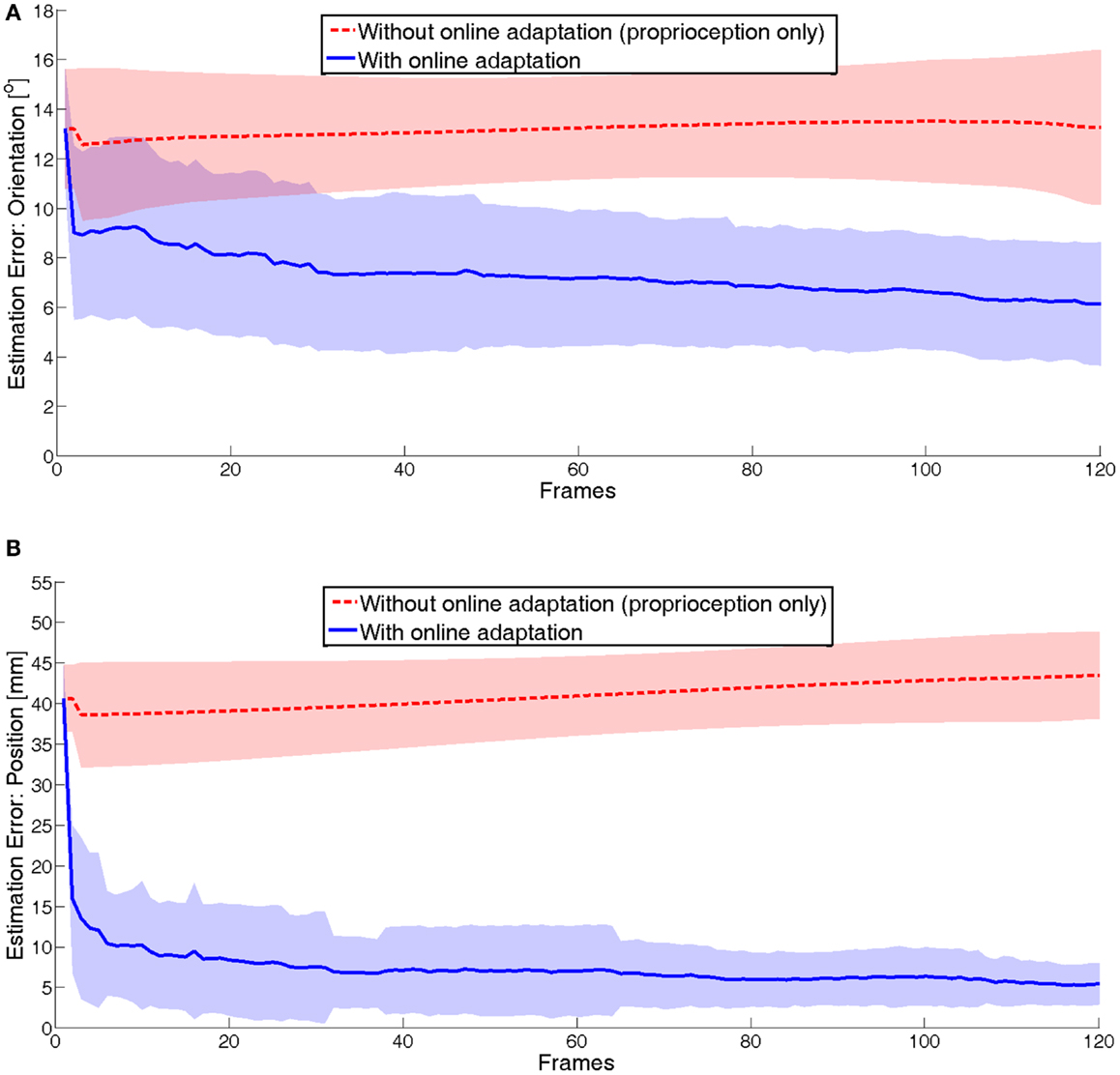
Figure 6. Estimation error of the end-effector during the open-loop phase: (A) orientation and (B) position.

In Figure 7, the evolution of the reaching error [see equation (39)] during the whole movement (open-loop and closed-loop) is displayed. Both the mean and the variance of the error over the 40 movements are shown. The high variance at the beginning of the motion is due to different (10) initial poses of the end-effector; some of them are closer (~60 mm) to the target pose than others (~120 mm). During the reaching movement, this variance reduces as the arm goes to the different (4) target poses; the variance is due to different arm configuration with constant artificial joint offsets.

FIGURE 7

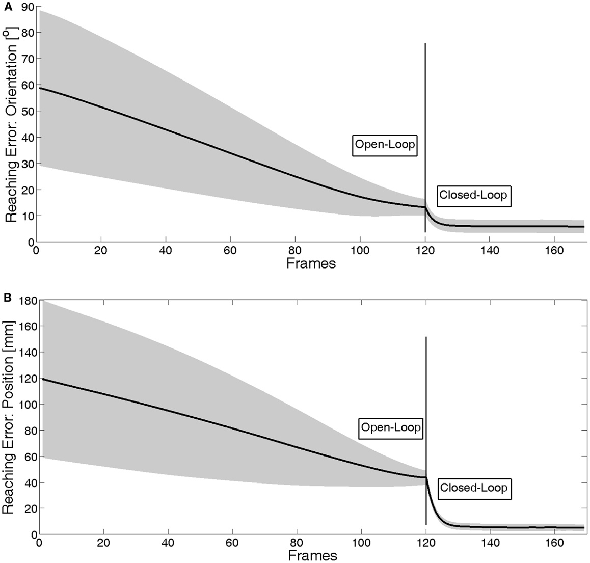
Figure 7. Real reaching error during the whole movement: (A) orientation and (B) position. The error is the average over 120 experiments: 4 different final poses, 10 different initial poses and each movement is repeated three times. It can be seen how the closed-loop correction considerably reduces the reaching error.

The open-loop part of the movement is planned at the movement onset, based on the non-calibrated model. Therefore, the reaching error at the end of the open-loop phase is equal to the pose estimation error with the non-calibrated system (as it can be seen by comparing the red dotted lines in Figure 6) to the line in Figure 7 at frame 120, for both position and orientation. Then, the body schema adaptation performed during the open-loop phase can be exploited at the onset of the closed-loop phase to obtain an accurate estimate of the pose of the end-effector; this allows to consistently reduce the reaching error already at frame 130. However, as expected, the error does not converge to 0 because there is still a residual error in the estimation of the end-effector pose (that can be appreciated in the blue bold line of the plot in Figure 6). Figure 8 shows a close-up of the final frames of the movement. The estimated reaching error (the dotted green line) converges indeed to 0, indicating that the closed-loop control is working properly. However, as mentioned above, the real reaching error (black solid line, same information as in Figure 7) does not converge, due to the residual estimation errors.

FIGURE 8

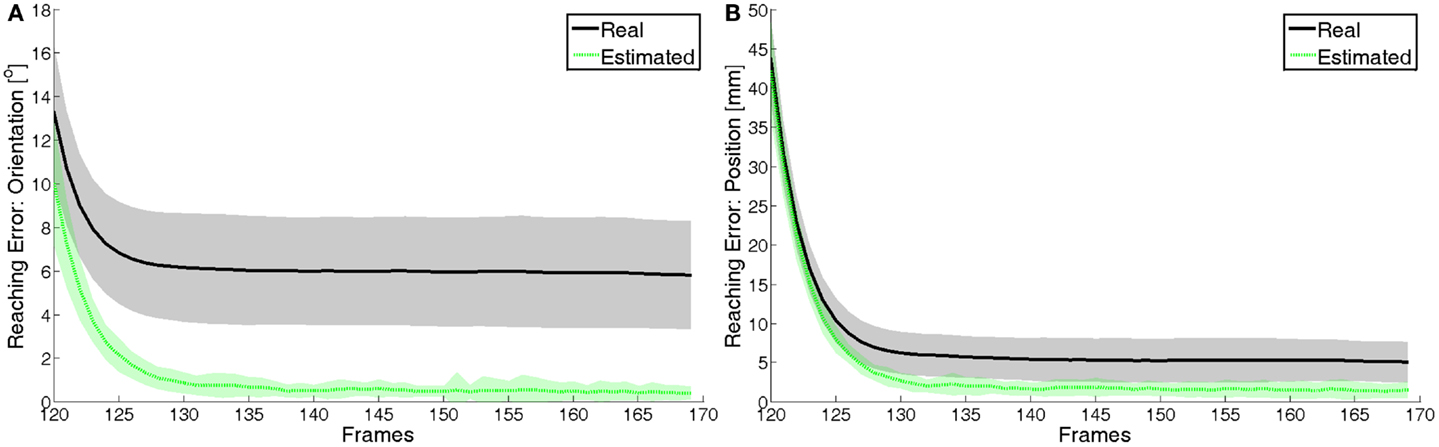
Figure 8. Real and estimated reaching error in the closed-loop phase: (A) orientation and (B) position. In black (solid), we can see the real reaching error and, in green (dotted), we can see the estimated reaching error. The latter converges to 0 as expected, proving that the closed-loop control is working properly.

Table 1 reports the exact numerical data related to the plots in Figures 6 and 7: the pose estimation error at the end of the open-loop phase (both with and without online adaptation) and the reaching error (both at the end of the open-loop and at the end of the closed-loop).

TABLE 1

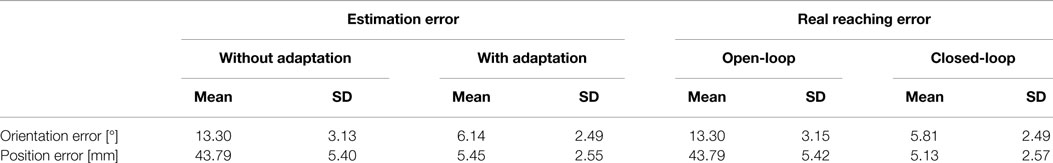
Table 1. Estimation and real reaching errors in the final poses of each movement: the estimation errors and the real reaching errors of open-loop are computed at frame 120, in the final pose of the open-loop phase.

5.1.2. Trade-Off between the Number of Particles and Estimation Accuracy

To generate particles/images and to compare them online with the ones obtained from visual feedback requires a lot of computational effort in the two processing units (Central Processing Unit (CPU) and Graphical Processing Unit (GPU)); therefore, the overall computational burden increases with the number of particles used in the SMC method. In order to better understand how the number of particles influences the accuracy of the estimation, we performed an extensive evaluation in which several movements are executed and the body schema adaptation is performed using different amounts of particles: M = 100; 200; 500; 1000; 2000. For each value of M, we perform 40 different movements with different initial and final poses. In each experiment, we maintain the parameters defined before in Section “Experimental settings” and we change only the amount of particles used; we performed the same motions of the right arm with the same visual feedback. The final end-effector pose estimation errors (mean and SD over the 40 movements) for each value of M are shown in Figure 9; then, in Table 2 we report only the mean values, and we compare them to the non-adaptation case as well. A clear trend can be noticed, which relates the increase of the number of particles to the decrease of the estimation error. However, this relation is non-linear: the slope of the curve is higher in the beginning and lower in the end. Indeed, the difference between the use of M = 1000 and M = 2000 is quite small, which suggests that further increasing the number of particles would not improve the estimation considerably. Moreover, it can be noticed that the estimation of the end-effector orientation benefits more of the increasing number of particles than the estimation of the end-effector position; this might be an indication that the orientation is more difficult to estimate.

FIGURE 9

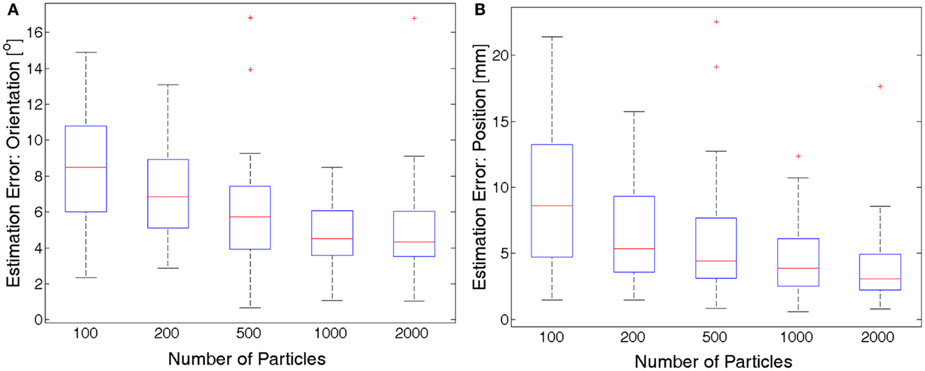
Figure 9. Comparing the final estimation error (orientation (A) and position (B)) using different amount of particles. The mean value of the error over 40 movements is shown. The accuracy increases with the number of particle used in anon-linear way, and it seems to stabilize after 1000 particles.

TABLE 2

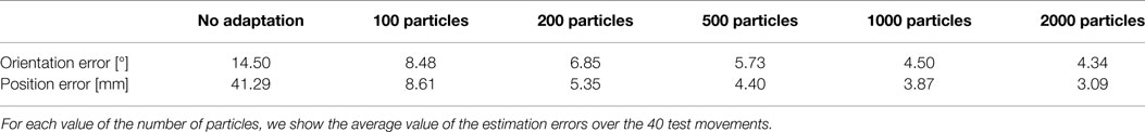
Table 2. Trade-off between number of particles and accuracy of the estimation.

In Figure 10, we show the temporal evolution of the pose estimation error during the arm movement in two representative cases: with M = 200 and M = 2000 particles. Although the orientation and position errors are smaller in the 2000 particles case, more computation is required with respect to the case with 200 particles (computation takes about 10 times longer). The time needed to generate and evaluate 200 particles is around 0.8 s per frame, while for 2000 particles is 7.5 s per frame. In other words, more time is needed to generate and evaluate the hypotheses and, therefore, the movement must be slower if we want to acquire the same number of frames/images.

FIGURE 10

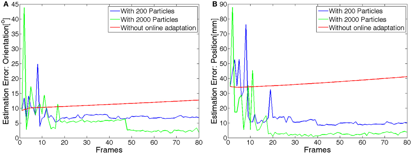
Figure 10. Evolution of the estimation error (orientation (A) and position (B)) for the non-calibrated system and for the system with online estimation performed with either 200 or 2000 particles. The mean value of the error over 40 movements is shown.

In summary, there is a trade-off between the accuracy of the estimation and the computation time for each iteration. In order to be able to perform the end-effector pose estimation in real-time in our current computer system, we chose to use M = 200 particles; this choice allows us to perform the estimation during reaching movements performed at natural speed (i.e., in the order of 0.01 m/s measured on the end-effector), with an average estimation error of about 5.35 mm in position and 6.85° in orientation.

5.2. Real Robot Results

In the real-world experiments, we use the real iCub as robot (see Figure 1) and a Unity^® computer graphics model as internal mental simulation.

Unity^® is a renowned cross-platform game engine developed by Unity Technologies that can generate very realistic virtual images. While the iCub Simulator uses simplified meshes of the robot external surfaces, our Unity model of the iCub renders the full CAD model of the robot, thus providing a much better match of the real robot appearance; in particular, for our experiments, a good appearance model of the robot hands is crucial. To perform the internal mental simulation process in real-time, we rely on GPU programing to achieve faster computation, as described in details in Vicente et al. (2015). Moreover, at each time instant we render only the robot parts that are visible by the robot cameras using a shader in the graphics pipeline, instead of rendering the whole robot appearance. A hierarchical tree of the robot kinematics is defined where each node has a reference frame attached and a pivot point that is used to perform the rotation of this hierarchical object structure (See Figure 11). In other words, this tree represents the relationship between the several objects in the model (i.e., the robot body parts). For instance, the fingers are coupled with the robot hand, so that if the hand moves, the fingers will move along with it and update their absolute position in the world, maintaining the relative pose in the hand reference frame.

FIGURE 11

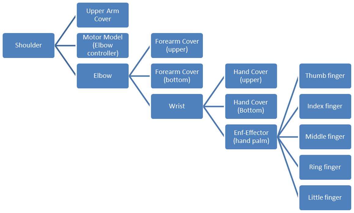
Figure 11. Hierarchical tree with the most important Unity Objects from the shoulder to the fingers.

In these experiments, we exploit the edge-based approach for the hand visual perception, described in Section “Edge extraction approach.” The silhouette approach that we used in the simulation experiments is not suitable in real-world scenarios due to the non-homogeneous background in the images, which makes segmentation difficult and noisy.

We maintain the initialization parameters defined in Section “Experimental Settings” and we define the tuning parameter of the edge distance as λ_edge = 0.01. This results in a higher likelihood when the distance of the nearest edge is around 1 pixel and a likelihood close to 0 when the distance reaches its maximum value (255).

As a way to evaluate the performance of the method in a real environment, we have chosen to use the left and right hands and apply the end-effector pose estimation on both. The goal is to get the hands close to each other with the index fingers almost touching. To achieve that the desired poses of the left and right end-effectors (i.e., the left and right hand palms) are defined with the same orientations, and with positions that differ only in the X-axis, of 12 cm; the fingers are slightly bent, so that the fingertips would touch when the hands are facing each other 12 cm apart. The target pose was chosen to be close to the center of both cameras for visualization purposes; however, this method can be applied in every location of the robot workspace, as long as the hands are in the field of view of one of the cameras. Therefore, the results shown are not specific to this target pose and similar experiments can be performed in any other configuration.

The robot starts from the home position seen in Figure 12. The left arm moves to the desired pose x^d and the target pose for the end-effector of the right arm is defined to have the same orientation of the left arm end-effector and a distance in the perpendicular direction of the palm of 12 cm.

FIGURE 12

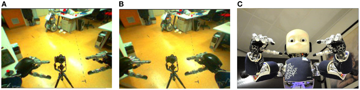
Figure 12. Body schema online adaptation performed in the real robot. Images seen by the robot eye cameras Left (A) and Right (B) Cameras and by an external camera (C) placed in front of the robot. Initial robot configuration.

In the first part of the experiment, we control both the left and the right arms to the desired end-effector poses, with open-loop control, performing the body schema adaptation and the estimation of the poses of the end-effectors. In the second part of the experiment, we control the pose of both end-effectors to the desired poses with closed-loop control, exploiting the adapted body schema and the improved pose estimation. In Figure 13, we show the comparison between the non-calibrated case (after the open-loop control, top row), where the hands have a distance from each other of approximately 16 cm and the fingertips are not aligned, and the adaptation performed using our method (with the closed-loop control, bottom row), where the hands are about 12 cm apart and the fingertips are touching each other (as desired).

FIGURE 13

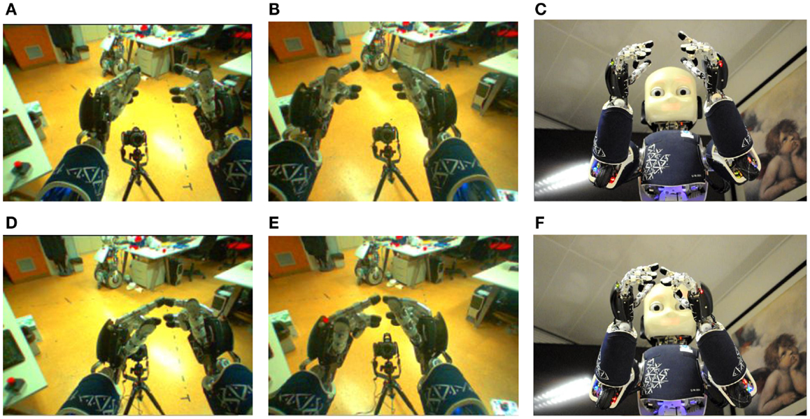
Figure 13. Body schema online adaptation performed in the real robot. Images seen by the robot eye cameras Left (A,D) and Right (B,E) Cameras and by external camera (C,F) placed in front of the robot. First row (A–C): the left arm is controlled toward a target end-effector pose and the right arm is controlled toward the same end-effector pose with a shift of 12 cm, with open-loop control. However, the resulting end-effector poses are not the desired one, due to inaccuracies in the body schema. Adaptation parameters are estimated during the motion of both arms, and used to update the body schema. Second row (D–F): the pose of both end-effectors is corrected using the updated body schema and a closed-loop control strategy that exploits the improved pose estimation.

6. Discussion

We have reported results both in simulation and in the real robot. The former constitute a quantitative evaluation with respect to ground-truth data; the latter demonstrate that the system can be used in the real world successfully. Indeed, in both cases, we achieve good results showing that both the estimation and reaching errors are decreased. Our approach is biologically inspired as evidence in neuroscience suggests that the human brain keeps an updated representation of the body (i.e., a body schema) that is employed to generate hypotheses of the limbs positions in space, which are combined with the actual perception of the self in a Bayesian fashion. Our system outperforms the current state of the art in the sense that (i) it does not rely on markers on the end-effector, using the pure visual feedback coming from the robot stereo cameras, (ii) the body schema adaptation is performed during reaching movements without a specific adaptation procedure, and (iii) such adaptation is performed online in real-time. While the body schema adaptation and pose estimation can be performed during each reaching movement, the adaptation parameters obtained during one movement generalize well to other areas of the workspace. This has been extensively documented in a previous publication (Vicente et al., 2015), in which we also show that our choice of parameterization (i.e., offsets in the arm joints) outperforms other solutions proposed in the literature, such as the use of offsets in the Cartesian position and orientation of the end-effector.

In general, the scalability of systems depends on the size of the search space (i.e., the parameters space). The fact that we parameterize the model with the joint offsets does not mean that other sources of error could not be accounted for. In theory, with a sufficient number of particles (and with a sufficient number of examples) any kind of error that causes a mismatch between the kinematic model and the real robot (e.g., unalignment of one joint axis of rotation, change in the length of one link, change in the elastic properties of one transmission cable) can be compensated for, since our sequential Monte Carlo parameter optimization approach attempts to minimize the prediction error between the body schema hypothesis and the visual perception. Although a quantitative analysis of the estimation with different error sources was not performed in this paper, the encouraging results obtained on the real robot (where other error sources than joint offsets are likely to be present) suggest that our system could deal with them.

The results provided in Section “Trade-Off between the Number of Particles and Estimation Accuracy” show that increasing the number of particles would lead to better estimation performance; however, the computational burden would also increase considerably. Interestingly, our architecture for the internal mental simulation could be easily made parallel to increase the computation speed. In the current system, one computer generates multiple hypotheses based on a single internal model; the number of generated hypothesis is the same of the number of particles. The hypothesis is then compared to the robot visual perception. The use of a big cluster of computers in which each machine runs an instance of the internal model and generates only a single hypothesis would considerably reduce the computation time, allowing to use a high number of particles (at the cost of using a high number of computers).

Our proposed solution is not robot-dependent, and can be applied to other robotic platforms in a straightforward manner, provided that a kinematic and graphical (texture) model of the robot is available. Clearly, the more the texture model of the robot is close to the real robot appearance, the better the estimation performance is expected to be. This is because in our current solution the appearance of the internal model is not updated exploiting the visual information gathered by the robot: only the kinematic structure is adapted based on the mismatch between the internal model predictions and the visual feedback.

7. Conclusion and Future Work

We presented a novel system for simultaneous online body schema adaptation and end-effector pose estimation implemented on the iCub humanoid robot. The parameter adaptation is performed with a sequential Monte Carlo framework during the execution of reaching movements. We rely only on the robot embedded sensors (vision sensing from stereo cameras and proprioception) without using any special visual marker. Our method draws inspiration from human perception and learning, as we combine the prediction made by a learned internal model with the actual visual feedback to improve the perceptual skill of the robot.

Overall, our simulation experiments show that we can reduce the end-effector pose estimation error considerably with respect to using the nominal (non-calibrated) robot model (of about eight times in the end-effector position and 2.2 times in the end-effector orientation). Moreover, the use of a closed-loop correction after the initial open-loop reaching motion (during which the body schema adaptation and pose estimation are performed) allows to reduce the reaching error of about 8.5 times in position and 2.3 times in orientation.

We demonstrated the applicability of our system to real-world scenarios by performing a bimanual reaching task with the real iCub robot, where the combined open-loop and closed-loop control strategy, made possible by the accurate pose estimation, allowed to decrease the positioning error of both end-effectors by 4 cm.

Some possible directions for the future work have been discussed in Section “Discussion.” Moreover, an interesting improvement to increase the robustness of the edge matching would be to use also the orientation of the matching edge on the model and compare its location and orientation with an edge in the realistic platform sensing information.

Author Contributions

In this work, all the authors contributed to the conception of an online body schema adaptation solution and to the analysis and interpretation of the data acquired.

Conflict of Interest Statement

The authors declare that the research was conducted in the absence of any commercial or financial relationships that could be construed as a potential conflict of interest.

Acknowledgments

This work was partially supported by Fundação para a Ciência e a Tecnologia [UID/EEA/50009/2013] and the European Projects POETICON++ [FP7-ICT-288382] and LIMOMAN [PIEF-GA-2013-628315].

Footnote

1. ^In other words, x and y belong to a generative model also known as hidden Markov model.

References

Agin, G. (1980). Computer vision systems for industrial inspection and assembly. IEEE Comput. 13, 11–20. doi: 10.1109/MC.1980.1653613

CrossRef Full Text | Google Scholar

Agravante, D., Pages, J., and Chaumette, F. (2013). “Visual servoing for the REEM humanoid robot’s upper body,” in IEEE-RAS International Conference on Robotics and Automation (ICRA) (Karlsruhe: IEEE), 5253–5258.

Google Scholar

Ashmead, D., McCarty, M., Lucas, L., and Belvedere, M. (1993). Visual guidance in infants’ reaching toward suddenly displaced targets. Child Dev. 64, 1111–1127. doi:10.1111/j.1467-8624.1993.tb04190.x

CrossRef Full Text | Google Scholar

Berlucchi, G., and Aglioti, S. (1997). The body in the brain: neural bases of corporeal awareness. Trends Neurosci. 20, 560–564. doi:10.1007/s00221-009-1970-7

PubMed Abstract | CrossRef Full Text | Google Scholar

Birbach, O., Bäuml, B., and Frese, U. (2012). “Automatic and self-contained calibration of a multi-sensorial humanoid’s upper body,” in IEEE-RAS International Conference on Robotics and Automation (ICRA) (Saint Paul, MN: IEEE), 3103–3108.

Google Scholar

Bohg, J., Morales, A., Asfour, T., and Kragic, D. (2014). Data-driven grasp synthesis – a survey. IEEE Trans. Robot. 30, 289–309. doi:10.1109/TRO.2013.2289018

CrossRef Full Text | Google Scholar

Borgefors, G. (1986). Distance transformations in digital images. Comput. Vis. Graph. Image Process. 34, 344–371. doi:10.1016/S0734-189X(86)80047-0

CrossRef Full Text | Google Scholar

Borgefors, G. (1988). Hierarchical chamfer matching: a parametric edge matching algorithm. IEEE Trans. Pattern Anal. Mach. Intell. 10, 849–865. doi:10.1109/34.9107

CrossRef Full Text | Google Scholar

Bushnell, E. (1985). The decline of visually guided reaching during infancy. Infant Behav. Dev. 8, 139–155. doi:10.1016/S0163-6383(85)80002-3

CrossRef Full Text | Google Scholar

Caligiore, D., Parisi, D., and Baldassarre, G. (2014). Integrating reinforcement learning, equilibrium points, and minimum variance to understand the development of reaching: a computational model. Psychol. Rev. 121, 389–421. doi:10.1037/a0037016

PubMed Abstract | CrossRef Full Text | Google Scholar

Canny, J. (1986). A computational approach to edge detection. IEEE Trans. Pattern Anal. Mach. Intell. 8, 679–698. doi:10.1109/TPAMI.1986.4767851

PubMed Abstract | CrossRef Full Text | Google Scholar

Chaumette, F., and Hutchinson, S. (2006). Visual servo control, part I: basic approaches. IEEE Robot. Autom. Mag. 13, 82–90. doi:10.1109/MRA.2006.250573

CrossRef Full Text | Google Scholar

Chaumette, F., and Hutchinson, S. (2007). Visual servo control, part II: advanced approaches. IEEE Robot. Autom. Mag. 14, 109–118. doi:10.1109/MRA.2007.339609

CrossRef Full Text | Google Scholar

Ciancio, A., Zollo, L., Guglielmelli, E., Caligiore, D., and Baldassarre, G. (2011). “Hierarchical reinforcement learning and central pattern generators for modeling the development of rhythmic manipulation skills,” in IEEE International Conference on Development and Learning (ICDL), Vol. 2 (Frankfurt: IEEE), 1–8.

Google Scholar

Ciliberto, C., Smeraldi, F., Natale, L., and Metta, G. (2011). “Online multiple instance learning applied to hand detection in a humanoid robot,” in IEEE/RSJ International Conference on Intelligent Robots and Systems (IROS) (San Francisco, CA: IEEE), 1526–1532.

Google Scholar

Ciocarlie, M., Hsiao, K., Jones, E. G., Chitta, S., Rusu, R. B., and Sucan, I. A. (2010). “Towards reliable grasping and manipulation in household environments,” in Internacional Symposium on Experimental Robotics (ISER) (New Delhi: Springer), 241–252.

Google Scholar

Comport, A., Marchand, E., Pressigout, M., and Chaumette, F. (2006). Real-time markerless tracking for augmented reality: the virtual visual servoing framework. IEEE Trans. Vis. Comput. Graph 12, 615–628. doi:10.1109/TVCG.2006.78

PubMed Abstract | CrossRef Full Text | Google Scholar

Cox, T. F., and Cox, M. (2000). Multidimensional Scaling, 2 Edn. New York: Chapman and Hall/CRC.

Google Scholar

Damas, B., Jamone, L., and Santos-Victor, J. (2013). “Open and closed-loop task space trajectory control of redundant robots using learned models,” in IEEE/RSJ International Conference on Intelligent Robots and Systems (IROS) (Tokyo: IEEE), 163–169.

Google Scholar

Erol, A., Bebis, G., Nicolescu, M., Boyle, R. D., and Twombly, X. (2007). Vision-based hand pose estimation: a review. Comput. Vis. Image Understand. 108, 52–73. doi:10.1016/j.cviu.2006.10.012

CrossRef Full Text | Google Scholar

Fanello, S. R., Pattacini, U., Gori, I., Tikhanoff, V., Randazzo, M., Roncone, A., et al. (2014). “3D stereo estimation and fully automated learning of eye-hand coordination in humanoid robots,” in IEEE-RAS International Conference on Humanoid Robots (Madrid: IEEE), 1028–1035.

Google Scholar

Figueiredo, R., Shukla, A., Aragao, D., Moreno, P., Bernardino, A., Santos-Victor, J., et al. (2012). “Reaching and grasping kitchenware objects,” in IEEE/SICE International Symposium on System Integration (SII) (Fukuoka: IEEE), 865–870.

Google Scholar

Friston, K. (2010). The free-energy principle: a unified brain theory? Nat. Rev. Neurosci. 2, 127–138. doi:10.1038/nrn2787

PubMed Abstract | CrossRef Full Text | Google Scholar

Gratal, X., Romero, J., and Kragic, D. (2011). “Virtual visual servoing for real-time robot pose estimation,” in 18th World Congress of the International Federation of Automatic Control (Milano: IFAC), 9017–9022.

Google Scholar

Hoffmann, M., Marques, H., Hernandez Arieta, A., Sumioka, H., Lungarella, M., and Pfeifer, R. (2010). Body schema in robotics: a review. IEEE Trans. Autonom. Ment. Dev. 2, 304–324. doi:10.1109/TAMD.2010.2086454

CrossRef Full Text | Google Scholar

Hol, J., Schon, T., and Gustafsson, F. (2006). “On resampling algorithms for particle filters,” in IEEE Nonlinear Statistical Signal Processing Workshop (Cambridge: IEEE), 79–82.

Google Scholar

Hutchinson, S., Hager, G., and Corke, P. (1996). A tutorial on visual servo control. IEEE Trans. Robot. Autom. 12, 651–670. doi:10.1109/70.538972

CrossRef Full Text | Google Scholar

Jamone, L., Damas, B., Endo, N., Santos-Victor, J., and Takanishi, A. (2013a). Incremental development of multiple tool models for robotic reaching through autonomous exploration. PALADYN J. Behav. Robot. 03, 113–127. doi:10.2478/s13230-013-0102-z

CrossRef Full Text | Google Scholar

Jamone, L., Damas, B., Santos-Victor, J., and Takanishi, A. (2013b). “Online learning of humanoid robot kinematics under switching tools contexts,” in IEEE-RAS International Conference on Robotics and Automation (ICRA) (Karlsruhe: IEEE), 4811–4817.

Google Scholar

Jamone, L., Natale, L., Hashimoto, K., Sandini, G., and Takanishi, A. (2011). “Learning task space control through goal directed exploration,” in IEEE International Conference on Robotics and Biomimetics (ROBIO) (Phuket: IEEE), 702–708.

Google Scholar

Jamone, L., Natale, L., Nori, F., Metta, G., and Sandini, G. (2012). Autonomous online learning of reaching behavior in a humanoid robot. Int. J. HR 09, 1250017. doi:10.1142/S021984361250017X

CrossRef Full Text | Google Scholar

Joseph, R. (2000). Fetal brain behavior and cognitive development. Dev. Rev. 20, 81–98. doi:10.1006/drev.1999.0486

CrossRef Full Text | Google Scholar

Kantas, N., Doucet, A., Singh, S., and Maciejowski, J. (2009). “An overview of sequential monte carlo methods for parameter estimation on general state space models,” in IFAC Symposium on System Identification (SYSID) (Saint Malo: IFAC), 774–785.

Google Scholar

Körding, K. P., and Wolpert, D. M. (2004). Bayesian integration in sensorimotor learning. Nature 427, 244–247. doi:10.1038/nature02169

PubMed Abstract | CrossRef Full Text | Google Scholar

Kulpate, C., Mehrandezh, M., and Paranjape, R. (2005). “An eye-to-hand visual servoing structure for 3d positioning of a robotic arm using one camera and a flat mirror,” in IEEE/RSJ International Conference on Intelligent Robots and Systems (IROS) (Alberta: IEEE), 1464–1470.

Google Scholar

La Anh, T., and Song, J.-B. (2012). Robotic grasping based on efficient tracking and visual servoing using local feature descriptors. Int. J. Precis. Eng. Manuf. 13, 387–393. doi:10.1007/s12541-012-0049-8

CrossRef Full Text | Google Scholar

Leitner, J., Harding, S., Frank, M., Forster, A., and Schmidhuber, J. (2013). “Humanoid learns to detect its own hands,” in IEEE Congress on Evolutionary Computation (CEC) (Cancun: IEEE), 1411–1418.

Google Scholar

Lockman, J. J., Ashmead, D. H., and Bushnell, E. W. (1984). The development of anticipatory hand orientation during infancy. J. Exp. Child Psychol. 37, 176–186. doi:10.1016/0022-0965(84)90065-1

PubMed Abstract | CrossRef Full Text | Google Scholar

Ma, G., Huang, Q., Yu, Z., Chen, X., Meng, L., Sultan, M., et al. (2013). “Hand-eye servo and flexible control of an anthropomorphic arm,” in IEEE International Conference on Robotics and Biomimetics (ROBIO) (Shenzhen: IEEE), 1432–1437.

Google Scholar

Mathew, A., and Cook, M. (1990). The control of reaching movements by young infants. Child Dev. 61, 1238–1257. doi:10.2307/1130891

PubMed Abstract | CrossRef Full Text | Google Scholar

Metta, G., Natale, L., Nori, F., Sandini, G., Vernon, D., Fadiga, L., et al. (2010). The icub humanoid robot: an open-systems platform for research in cognitive development. Neural Netw. 23, 1125–1134. doi:10.1007/978-3-540-77296-5_32

PubMed Abstract | CrossRef Full Text | Google Scholar

Miall, R. C., and Wolpert, D. M. (1996). Forward models for physiological motor control. Neural Netw. 9, 1265–1279. doi:10.1016/S0893-6080(96)00035-4

CrossRef Full Text | Google Scholar

Moutinho, N., Brandao, M., Ferreira, R., Gaspar, J., Bernardino, A., Takanishi, A., et al. (2012). “Online calibration of a humanoid robot head from relative encoders, imu readings and visual data,” in IEEE/RSJ International Conference on Intelligent Robots and Systems (IROS) (Vilamoura: IEEE), 2070–2075.

Google Scholar

Pattacini, U. (2011). Modular Cartesian Controllers for Humanoid Robots: Design and Implementation on the iCub. Ph.D. thesis, Italian Institute of Technology, Genoa.

Google Scholar

Peniak, M., and Cangelosi, A. (2014). “Scaling-up action learning neuro-controllers with GPUs,” in International Joint Conference on Neural Networks (IJCNN) (Beijing: IEEE), 2519–2524.

Google Scholar

Reinhart, R., and Steil, J. (2009). “Reaching movement generation with a recurrent neural network based on learning inverse kinematics for the humanoid robot icub,” in 9th IEEE-RAS International Conference on Humanoid Robots (Humanoids) (Paris: IEEE), 323–330.

Google Scholar

Rochat, P. (1998). Self-perception and action in infancy. Exp. Brain Res. 123, 102–109. doi:10.1007/s002210050550

PubMed Abstract | CrossRef Full Text | Google Scholar

Rolf, M. (2013). “Goal babbling with unknown ranges: a direction-sampling approach,” in IEEE Joint International Conference on Development and Learning and Epigenetic Robotics (ICDL-Epirob) (Osaka: IEEE), 1–7.

Google Scholar

Rolf, M., Steil, J., and Gienger, M. (2010). Goal babbling permits direct learning of inverse kinematics. IEEE Trans. Autonom. Ment. Dev. 2, 216–229. doi:10.1109/TAMD.2010.2062511

CrossRef Full Text | Google Scholar

Saxena, A., Driemeyer, J., and Ng, A. Y. (2008). Robotic grasping of novel objects using vision. Int. J. Rob. Res. 27, 157–173. doi:10.1177/0278364907087172

CrossRef Full Text | Google Scholar

Siciliano, B., and Khatib, O. (2007). Springer Handbook of Robotics. New York: Springer-Verlag.

Google Scholar

Sober, S. J., and Sabes, P. N. (2005). Flexible strategies for sensory integration during motor planning. Nat. Neurosci. 8, 490–497. doi:10.1038/nn1427

PubMed Abstract | CrossRef Full Text | Google Scholar

Thrun, S., Burgard, W., and Fox, D. (2005). Probabilistic Robotics (Intelligent Robotics and Autonomous Agents). Cambridge: The MIT Press.

Google Scholar

Tikhanoff, V., Fitzpatrick, P., Nori, F., Natale, L., Metta, G., and Cangelosi, A. (2008). “The icub humanoid robot simulator,” in IROS Workshop on Robot Simulators (Nice).

Google Scholar

Ulbrich, S., de Angulo, V., Asfour, T., Torras, C., and Dillmann, R. (2009). “Rapid learning of humanoid body schemas with kinematic bézier maps,” in IEEE-RAS International Conference on Humanoid Robots (Humanoids) (Paris: IEEE), 431–438.

Google Scholar

Ulbrich, S., de Angulo, V. R., Asfour, T., Torras, C., and Dillmann, R. (2012). General robot kinematics decomposition without intermediate markers. IEEE Trans. Neural Netw. Learn. Syst. 23, 620–630. doi:10.1109/TNNLS.2012.2183886

PubMed Abstract | CrossRef Full Text | Google Scholar

Vahrenkamp, N., Wieland, S., Azad, P., Gonzalez, D., Asfour, T., and Dillmann, R. (2008). “Visual servoing for humanoid grasping and manipulation tasks,” in IEEE-RAS International Conference on Humanoid Robots (Daejeon: IEEE), 406–412.

Google Scholar

Van der Meer, A. (1997). Keeping the arm in the limelight: advanced visual control of arm movements in neonates. Eur. J. Paediatr. Neurol. 1, 103–108. doi:10.1016/S1090-3798(97)80040-2

PubMed Abstract | CrossRef Full Text | Google Scholar

Vicente, P., Ferreira, R., Jamone, L., and Bernardino, A. (2014). “Eye-hand online adaptation during reaching tasks in a humanoid robot,” in IEEE International Conferences on Development and Learning and Epigenetic Robotics (ICDL-Epirob) (Genoa: IEEE), 175–180.

Google Scholar

Vicente, P., Ferreira, R., Jamone, L., and Bernardino, A. (2015). “Gpu-enabled particle based optimization for robotic-hand pose estimation and self-calibration,” in IEEE International Conference on Autonomous Robot Systems and Competitions (ICARSC) (Vila Real: IEEE), 3–8.

Google Scholar

von Hofsten, C. (1991). Structuring of early reaching movements: a longitudinal study. J. Mot. Behav. 23, 280–292. doi:10.1080/00222895.1991.9942039

PubMed Abstract | CrossRef Full Text | Google Scholar

von Hofsten, C. (2004). An action perspective on motor development. Trends Cogn. Sci. 8, 266–272. doi:10.1016/j.tics.2004.04.002

PubMed Abstract | CrossRef Full Text | Google Scholar

Wolpert, D. M., Miall, R. C., and Kawato, M. (1998). Internal models in the cerebellum. Trends Cogn. Sci. 2, 338–347. doi:10.1007/978-94-007-1333-8_56

PubMed Abstract | CrossRef Full Text | Google Scholar

Appendix

Pseudo-code

In this appendix, we will give details on the implementations of some of the modules used in our approach. We show the pseudo-code of the most important modules developed.

We developed two modules: main module (Algorithm 1) and the internal mental simulation (Algorithm 2). In our work, they communicate via YARP middle-ware.

The main module is responsible for processing the images from the robot to generate the particles and updated their likelihood. Moreover, it publishes the estimated β that can be used to correct the end-effector pose. In the internal mental simulator, we generate the hypotheses and test them returning the likelihood of each particle.

ALGORITHM 1

ALGORITHM 1. Main module.

ALGORITHM 2

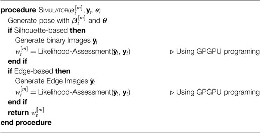
ALGORITHM 2. Internal mental simulator.