Set-Based Tasks within the Singularity-Robust Multiple Task-Priority Inverse Kinematics Framework: General Formulation, Stability Analysis, and Experimental Results

1. Introduction

The desired trajectory of robotic systems is typically given in the task space. In particular, this trajectory often describes the desired position trajectory of the end effector, which is then given in the Cartesian space. For control of robotic systems, the desired trajectory needs to be mapped from this task space to a reference trajectory in the joint space in which the actuators provide their input. In general, this topic falls within the inverse kinematics control problem. In most cases, the complexity of the problem requires numerical methods to solve the mapping (Siciliano et al., 2009).

Robotic systems with a large number of degrees of freedom (DOFs) are commonly used for industrial purposes (Siciliano et al., 2009) and are becoming increasingly important within a variety of domains, including humanoid robots (Escande et al., 2014) and unmanned vehicles, such as underwater (Simetti et al., 2013; Antonelli, 2014) and aerial systems (Baizid et al., 2015). Having developed beyond the structured and predictable industrial environment, robotic control algorithms are required to handle real-time trajectory generation. This requirement imposes the use of differential approaches for practical purposes, both at the kinematic and dynamic levels. In Whitney (1969), the use of the pseudoinverse is first recognized as a promising tool to solve the inverse kinematics problem at the kinematic level in robotic applications.

A robotic system is defined as redundant when it possesses more DOFs than those strictly required to solve its task, in which case-specific approaches need to be used (Chiaverini et al., 2008). Additional control possibilities then arise in terms of utilizing the “excess” DOFs by adding other tasks to be controlled simultaneously. This is an important possibility in unstructured or non-repetitive environments, as these require the algorithms to handle additional control objectives, such as staying within the mechanical joint limits, avoidance of obstacles, control of the orientation of directional sensors, and maximizing arm manipulability, in addition to the main control objectives. Note that joint limit tasks may be considered as a special case where the task space and the configuration space are identical. Hence, frameworks that map from configuration space to task space may still be utilized for these tasks.

In a task-priority framework, the different control objectives are embedded with a priority relative to their respective importance. The importance of prioritizing between the control objectives can arise from several reasons. Safety, for example, may be considered to be of supreme importance if the environment is shared with human operators. Thus, tracking of the end-effector trajectory may actually be assigned a lower priority in the rank of importance. These considerations lead to solutions as in Liégeois (1977), where the null-space projector is considered in the solution to achieve secondary control objectives afforded by a gradient-based approach. Secondary objectives are defined and handled in a task-priority approach in Maciejewski and Klein (1985) and Nakamura et al. (1987). The work (Siciliano and Slotine, 1991) extends this approach to multiple tasks. In Chiaverini (1997), a different approach is introduced, which guarantees singularity robustness with respect to algorithmic singularities. This approach is further extended to multiple tasks in priority and analyzed in Mansard and Chaumette (2007) and Antonelli (2009), and it is referred to as the singularity-robust multiple task-priority inverse kinematics framework.

Notice that the term hierarchy and priority are often used as synonyms in the literature. In this paper, the latter will be used.

The singularity-robust multiple task-priority inverse kinematics framework has been developed for equality tasks, which are tasks that assign an exact desired value to the controlled variable (e.g., the end-effector configuration). However, for a general robotic system, several goals may be described as set-based tasks, i.e., tasks with a desired interval [area of satisfaction (Escande et al., 2014)]. Two classic, yet vital examples are joint limits and obstacle avoidance. Additional examples are manipulability, dexterity, and field of view (for directional sensors, such as a camera mounted on the end effector). Set-based tasks are often referred to as inequality or unilateral constraints in the literature.

As recognized in Kanoun et al. (2011), inclusion of inequality constraints is still missing for the singularity-robust multiple task-priority inverse kinematics framework. This paper aims to fill that gap. In particular, in this paper, we will present a method that allows a general number of scalar set-based tasks to be handled with a given priority within a number of equality tasks. A preliminary description of the idea is given in Antonelli et al. (2015), and Moe et al. (2015a) present some experimental results of the proposed algorithm. It is worth noticing that, with respect to similar approaches presented in the literature, this is the very first one with a formal stability analysis, presented in Moe et al. (2015b). The contribution of this paper is to streamline and present the previous conference contributions in a unified manner and to address how set-based tasks that are given lower priority in the task hierarchy should be handled. Furthermore, new experimental results are presented.

This paper is organized as follows. Section 2 presents relevant literature and alternative approaches to handle set-based tasks. Section 3 gives a brief introduction to the singularity-robust multiple task-priority inverse kinematics framework that is the basis for the presented method, and a closer definition of set-based tasks. The proposed method is described in Section 4, both for high-priority and low-priority set-based tasks and a combination of the two, and it is analyzed with respect to stability in Section 5. Finally, Section 6 considers the practical implementation of the suggested algorithm, and Section 7 presents experimental results performed on a UR5 manipulator. Conclusion and future work are given in Section 8.

2. Relevant Literature

In Kanoun et al. (2011) and Simetti et al. (2013), it is pointed out that in order to handle set-based tasks, these are often transformed into equality constraints or un-proper potentials, which leads to over-constraining the original control problem.

One possible way to systematically handle tasks arranged in priority with set-based and equality objectives is to transform the inverse kinematics problem into a quadratic programing (QP) or a similar optimization problem (Ioannou and Sun, 1996), thereby preventing the tasks from being directly included in the multiple task-priority inverse kinematics algorithm unlike the approach suggested in this paper. One of the first solutions using this approach is given by Faverjon and Tournassoud (1987), generalized by Kanoun et al. (2011), and further improved by de Lasa et al. (2010) and Escande et al. (2014) in terms of convergence time. In de Lasa et al. (2010), however, set-based tasks can be considered only as high priority tasks. In Azimian et al. (2014), the inequality constrains are transformed to an equality constraint by the use of proper slack variables. The optimization problem is then modified in order to minimize the defined slack variables together with the task errors in a task-priority architecture.

Set-based tasks may also be embedded in the control problem by assigning virtual forces that push the robot away from the set boundaries. This idea was first proposed in Khatib (1986) and then used in several following approaches. However, when resorting to virtual forces/potentials, satisfaction of the boundaries can not be analytically guaranteed and often the overall control architecture falls within the paradigm of cooperative behavioral control, which is possibly affected with drawbacks described in Antonelli et al. (2008). In Simetti et al. (2013), there is a systematic method for handling set-based tasks within the framework of potential fields. In particular, the key aspect is to resort to finite-support smooth potential fields for representing set-based objectives and activation functions. Experimental results with an underwater vehicle-manipulator system are provided. During the activation of the smoothing functions, however, strict priority among the tasks is lost, which is a common drawback when smoothing functions are introduced to avoid discontinuities also in alternative approaches.

In Mansard et al. (2009), set-based tasks are handled within a framework of transitions between solutions. In particular, the transition is necessary to handle the unilateral constraint and avoid discontinuities. Using the damped least-square inverse of the Jacobian, the proposed algorithm does not respect priorities during transitions. In practice, the proposed solution is a way to handle the algorithm given in Siciliano and Slotine (1991) by resorting to homotopy.

In adaptive control, projection methods may be used to ensure that the parameter estimates are bounded by using projection methods (Ioannou and Sun, 1996). The method proposed in this paper may be considered as a type of projection method in the sense that we suggest a discontinuous solution for the system velocities based on projecting the solutions. We suggest a method to directly embed the set-based tasks into the singularity-robust multiple task-priority inverse kinematics framework, thereby making it unnecessary to rewrite the problem into an optimization problem or resort to potential fields. By including the set-based tasks directly into this framework, a stability analysis is feasible, and the paper presents a formal stability analysis with explicit assumptions. Furthermore, the strict priority of the tasks is fulfilled at all times.

3. Background

3.1. Singularity-Robust Multiple Task-Priority Inverse Kinematics

A general robotic system has n DOFs. Its configuration is given by the joint values q = [q₁, q₂, …, q_n]^T. It is then possible to express tasks and task velocities in the operational space through forward kinematics and the task Jacobian matrix. Let us define σ(t) ∈ ℝ^m as the task variable to be controlled:

$\mathit{\sigma }\left(t\right)=\mathit{f}\left(\mathit{q}\left(t\right)\right)$ (1)

with the corresponding differential relationship:

$\dot{\mathit{\sigma }}\left(t\right)=\frac{\partial \mathit{f}\left(\mathit{q}\left(t\right)\right)}{\partial \mathit{q}}\dot{\mathit{q}}\left(t\right)=\mathit{J}\left(\mathit{q}\left(t\right)\right)\dot{\mathit{q}}\left(t\right),$ (2)

where J(q(t)) ∈ ℝ^m×n is the configuration-dependent analytical task Jacobian matrix and $\dot{\mathit{q}}\left(t\right)\in {\mathbb{R}}^n$ is the system velocity. For compactness, the argument q of tasks and Jacobians are omitted from the equations in this paper.

Let us first consider a single m-dimensional task to be followed, with a defined desired trajectory σ_des(t) ∈ ℝ^m. The corresponding joint references q_des(t) ∈ ℝⁿ for the robotic system may be computed by integrating the locally inverse mapping of equation (2) achieved by imposing minimum-norm velocity (Siciliano, 1990). The following least-squares solution is given:

${\dot{\mathit{q}}}_{\text{des}}={\mathit{J}}^{†}{\dot{\mathit{\sigma }}}_{\text{des}}={\mathit{J}}^{\text{T}}{\left({\mathit{JJ}}^{\text{T}}\right)}^{-1}{\dot{\mathit{\sigma }}}_{\text{des}},$ (3)

where J^†, implicitly defined in the above equation for full row rank matrices, is the right pseudoinverse of J. In the general case, the pseudoinverse is the matrix that satisfies the four Moore–Penrose conditions [equations (4)–(7)] (Golub and Van Loan, 1996), and it is defined for systems that are not square (m ≠ n) nor have full rank (Buss, 2009):

${\mathit{JJ}}^{†}\mathit{J}=\mathit{J},$ (4)

${\mathit{J}}^{†}{\mathit{JJ}}^{†}={\mathit{J}}^{†},$ (5)

${\left({\mathit{JJ}}^{†}\right)}^{\star }={\mathit{JJ}}^{†},$ (6)

${\left({\mathit{J}}^{†}\mathit{J}\right)}^{\star }={\mathit{J}}^{†}\mathit{J}.$ (7)

Here, J* denotes the complex conjugate of J.

The vector q_des achieved by taking the time integral of equation (3) is prone to drifting. To handle this, a closed loop inverse kinematics (CLIK) version of the algorithm is usually implemented (Chiaverini, 1997), namely,

${\dot{\mathit{q}}}_{\text{des}}={\mathit{J}}^{†}\left({\dot{\mathit{\sigma }}}_{\text{des}}+\mathbf{\Lambda }\tilde{\mathit{\sigma }}\right)={\mathit{J}}^{†}{\dot{\mathit{\sigma }}}_{\text{ref}},$ (8)

where $\tilde{\mathit{\sigma }}\in {\mathbb{R}}^m$ is the task error defined as

$\tilde{\mathit{\sigma }}={\mathit{\sigma }}_{\text{des}}-\mathit{\sigma }$ (9)

and $\mathbf{\Lambda }\in {\mathbb{R}}^{m\times m}$ is a positive-definite matrix of gains. This feedback approach reduces the error dynamics to

$\begin{array}{l}\dot{\tilde{\mathit{\sigma }}}={\dot{\mathit{\sigma }}}_{\text{des}}-\dot{\mathit{\sigma }}={\dot{\mathit{\sigma }}}_{\text{des}}-\mathit{J}\dot{\mathit{q}}\hfill \\ ={\dot{\mathit{\sigma }}}_{\text{des}}-\mathit{J}{\mathit{J}}^{†}\left({\dot{\mathit{\sigma }}}_{\text{des}}+\mathbf{\Lambda }\tilde{\mathit{\sigma }}\right)\hfill \\ =-\mathbf{\Lambda }\tilde{\mathit{\sigma }},\hfill \end{array}$ (10)

if $\dot{\mathit{q}}={\dot{\mathit{q}}}_{\text{des}}$ and J has full rank, implying that JJ^† = I. Equation (10) describes a linear system with a globally exponentially stable equilibrium point at the equilibrium $\tilde{\mathit{\sigma }}=\mathit{0}$. It is worth noticing that the assumption $\dot{\mathit{q}}={\dot{\mathit{q}}}_{\text{des}}$ is common to all inverse kinematics algorithms (Antonelli, 2008). For practical applications, it requires that the low-level dynamic control loop is faster than the kinematic one.

In case of system redundancy, i.e., if n > m, the classic general solution contains a null projector operator (Liégeois, 1977):

${\dot{\mathit{q}}}_{\text{des}}={\mathit{J}}^{†}{\dot{\mathit{\sigma }}}_{\text{ref}}+\left({\mathit{I}}_n-{\mathit{J}}^{†}\mathit{J}\right){\dot{\mathit{q}}}_{\text{null}},$ (11)

where I_n is the (n × n) identity matrix and the vector ${\dot{\mathit{q}}}_{\text{null}}\in {\mathbb{R}}^n$ is an arbitrary system velocity vector. It can be recognized that the operator (I_n − J^† J) projects ${\dot{\mathit{q}}}_{\text{null}}$ in the null space of the Jacobian matrix. This corresponds to generating a motion of the robotic system that does not affect that of the given task.

For highly redundant systems, multiple tasks can be arranged in priority. Let us consider three tasks that will be denoted with the subscripts 1, 2 and 3, respectively:

${\mathit{\sigma }}_1={\mathit{f}}_1\left(\mathit{q}\right)\in {\mathbb{R}}^{m_1}$ (12)

${\mathit{\sigma }}_2={\mathit{f}}_2\left(\mathit{q}\right)\in {\mathbb{R}}^{m_2}$ (13)

${\mathit{\sigma }}_3={\mathit{f}}_3\left(\mathit{q}\right)\in {\mathbb{R}}^{m_3}.$ (14)

For each of the tasks, a corresponding Jacobian matrix can be defined, denoted J₁ ∈ ℝ^m₁×n, J₂ ∈ ℝ^m₂×n, and J₃ ∈ ℝ^m₃×n, respectively. Let us further define the corresponding null-space projectors for the first two tasks as

${\mathit{N}}_1=\left({\mathit{I}}_n-{\mathit{J}}_1^{†}{\mathit{J}}_1\right)$ (15)

${\mathit{N}}_2=\left({\mathit{I}}_n-{\mathit{J}}_2^{†}{\mathit{J}}_2\right).$ (16)

The augmented Jacobian of tasks 1 and 2 is given by stacking the two independent task Jacobians:

${\mathit{J}}_{12}^{\text{A}}=\left[\begin{array}{c}\hfill {\mathit{J}}_1\hfill \\ \hfill {\mathit{J}}_2\hfill \end{array}\right]$ (17)

The common null-space for tasks 1 and 2 is then defined as

${\mathit{N}}_{12}^{\text{A}}=\left({\mathit{I}}_n-{{\mathit{J}}_{12}^{\text{A}}}^{†}{\mathit{J}}_{12}^{\text{A}}\right),$ (18)

where ${{\mathit{J}}_{12}^{\text{A}}}^{†}$ is the pseudoinverse of ${\mathit{J}}_{12}^{\text{A}}$ that satisfies the four Moore–Penrose conditions [equations (4)–(7)]. By expanding the expression for ${\mathit{J}}_{12}^{\text{A}}$, we see that

$\begin{array}{l}\left[\begin{array}{c}{\mathit{J}}_1\\ {\mathit{J}}_2\end{array}\right]{\mathit{N}}_{12}^{\text{A}}=\left[\begin{array}{c}{\mathit{J}}_1\\ {\mathit{J}}_2\end{array}\right]\left({\mathit{I}}_n-{\left[\begin{array}{c}{\mathit{J}}_1\\ {\mathit{J}}_2\end{array}\right]}^{†}\left[\begin{array}{c}{\mathit{J}}_1\\ {\mathit{J}}_2\end{array}\right]\right)\hfill \\ =\left[\begin{array}{c}{\mathit{J}}_1\\ {\mathit{J}}_2\end{array}\right]-\left[\begin{array}{c}{\mathit{J}}_1\\ {\mathit{J}}_2\end{array}\right]{\left[\begin{array}{c}{\mathit{J}}_1\\ {\mathit{J}}_2\end{array}\right]}^{†}\left[\begin{array}{c}{\mathit{J}}_1\\ {\mathit{J}}_2\end{array}\right]\hfill \\ =\left[\begin{array}{c}{\mathit{J}}_1\\ {\mathit{J}}_2\end{array}\right]-\left[\begin{array}{c}{\mathit{J}}_1\\ {\mathit{J}}_2\end{array}\right]=\left[\begin{array}{c}\mathit{0}\\ \mathit{0}\end{array}\right],\hfill \end{array}$ (19)

so in general,

${\mathit{J}}_i{\mathit{N}}_{12..k}^{\text{A}}=\mathit{0}\text{for}i\in \left\{1,...,k\right\}.$ (20)

The following equation then defines the desired joint velocities:

${\dot{\mathit{q}}}_{\text{des}}=\underset{{\dot{\mathit{q}}}_{1,\text{des}}}{\underbrace{{\mathit{J}}_1^{†}{\dot{\mathit{\sigma }}}_{1,\text{ref}}}}+{\mathit{N}}_1\underset{{\dot{\mathit{q}}}_{2,\text{des}}}{\underbrace{{\mathit{J}}_2^{†}{\dot{\mathit{\sigma }}}_{2,\text{ref}}}}+{\mathit{N}}_{12}^{\text{A}}\underset{{\dot{\mathit{q}}}_{3,\text{des}}}{\underbrace{{\mathit{J}}_3^{†}{\dot{\mathit{\sigma }}}_{3,\text{ref}}}}$ (21)

where the definition of ${\dot{\mathit{\sigma }}}_{x,\text{ref}}$ can be easily extrapolated from equation (8) for each task with the corresponding positive-definite matrix ${\mathbf{\Lambda }}_x\in {\mathbb{R}}^{m_x\times m_x}$. The priority of the tasks follows the numerical order, with σ₁ being the highest-priority task. Equation (21) also implicitly defines the joint velocities ${\dot{\mathit{q}}}_{x,\text{des}}\in {\mathbb{R}}^n$ that represent the desired joint velocity corresponding to task σ_x if this was the sole task.

The generalization to k tasks is straightforward: equation (21) can be expanded as:

${\dot{\mathit{q}}}_{\text{des}}={\mathit{J}}_1^{†}{\dot{\mathit{\sigma }}}_{1,\text{ref}}+{\mathit{N}}_1{\mathit{J}}_2^{†}{\dot{\mathit{\sigma }}}_{2,\text{ref}}+\cdots +{\mathit{N}}_{12\dots \left(k-1\right)}^{\text{A}}{\mathit{J}}_k^{†}{\dot{\mathit{\sigma }}}_{k,\text{ref}}$ (22)

where ${\mathit{N}}_{12\dots \left(k-1\right)}^{\text{A}}$ is the null space of the augmented Jacobian matrix

${\mathit{J}}_{12\dots \left(k-1\right)}^{\text{A}}=\left[\begin{array}{c}\hfill {\mathit{J}}_1\hfill \\ \hfill {\mathit{J}}_2\hfill \\ \hfill ⋮\hfill \\ \hfill {\mathit{J}}_{k-1}\hfill \end{array}\right].$ (23)

3.2. Set-Based Definitions

The previous section introduced the concept of multiple task-priority inverse kinematic control for a robotic system, as a method to generate reference trajectories for the system configuration that, if satisfied, will result in the successful achievement of several tasks. However, this framework has been developed for equality tasks that have a specific desired value σ_des(t), e.g., the desired end effector position. This paper proposes a method to extend the existing framework to handle set-based tasks, such as the avoidance of joint limits and obstacles, and field of view.

A set-based task is still expressed through forward kinematics equation (1), but the objective is to keep the task in a defined set D rather than controlling it to a desired value. Mathematically, this can be expressed as σ(t) ∈ D ∀ t rather than σ(t) = σ_des(t). Thus, set-based tasks cannot be directly inserted into the singularity-robust multiple task-priority inverse kinematics framework [equation (22)]. In this paper, we will present a method that allows a general number of scalar set-based tasks to be handled with a given priority within a number of equality tasks.

From here on, equality tasks are denoted with number subscripts and set-based tasks with letters. Furthermore, while equality tasks in general can be multidimensional and are thus described as vectors, set-based tasks are scalar and are therefore not expressed in bold-face, e.g., σ₁ and σ_a. Finally, only regulation equality tasks are considered, that is equality tasks to guide the system to a stationary value (${\dot{\mathit{\sigma }}}_{\text{des}}\equiv 0$). Finally, it is assumed that the desired joint velocities ${\dot{\mathit{q}}}_{\text{des}}$ are tracked perfectly by the system, so that $\dot{\mathit{q}}={\dot{\mathit{q}}}_{\text{des}}$.

Consider Figure 1. A set-based task σ is defined as satisfied when it is contained in its valid set, i.e., σ ∈ D = [σ_min, σ_max]. On the boundary of D, the task is still satisfied, but it might be necessary to actively handle the task to prevent it from becoming violated. This is elaborated on in Section 4.

FIGURE 1

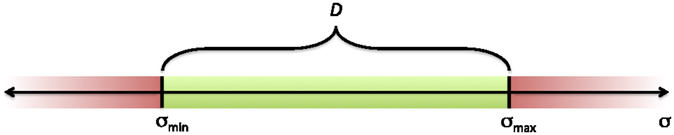
Figure 1. Illustration of valid set D. The set-based task σ is satisfied in D and violated outside of D.

4. Set-Based Singularity-Robust Task-Priority Inverse Kinematics

This section presents the proposed method for incorporating set-based tasks in the singularity-robust multiple task-priority inverse kinematics framework. High-priority set-based tasks are defined as all set-based tasks with a higher priority than the highest-priority equality task, whereas low-priority set-based tasks have priority after at least one equality task. Section 4.1 describes how high-priority set-based tasks are handled. For simplicity, a system with a single set-based task is considered first, before the general case of j set-based tasks is presented. Low-priority set-based tasks offer some additional challenges and are further described in Section 4.2, also for 1 and j set-based tasks, respectively. Finally, in Section 4.3, the framework is presented for the completely general case of a combination of high- and low-priority set-based tasks. Note that concrete examples are given in Section 7.

When a set-based task is in the interior of D (Figure 1), it should not affect the behavior of the system. All the system DOFs can then be used to fulfill the equality tasks without being limited in any way by the set-based task, which is inactive. The proposed algorithm therefore considers only the system’s equality tasks according to equation (33) as long as the resulting solution stays within this desired set or, should it be outside, does not further increase the distance to the set. If this is not the case, the set-based task is actively inserted into the task priority to be handled. A key aspect of the proposed solution is the tangent cone and extended tangent cone to a set. The tangent cone to the set D in Figure 1 at the point σ ∈ D is defined as

$T_D\left(\mathrm{\sigma }\right)=\left\{\begin{array}{cc}\left[0,\infty \right)\hfill & \mathrm{\sigma }={\mathrm{\sigma }}_{\text{min}}\hfill \\ \mathbb{R}\hfill & \mathrm{\sigma }\in \left({\mathrm{\sigma }}_{\text{min}},{\mathrm{\sigma }}_{\text{max}}\right)\hfill \\ \left(-\infty ,0\right]\hfill & \mathrm{\sigma }={\mathrm{\sigma }}_{\text{max}}\hfill \end{array}\right..$ (24)

The left-end point in Figure 1 corresponds to σ_min, in which case the tangent cone is defined as [0,∞). Similarly, the right-end point of Figure 1 represents σ_max, and in this point, the tangent cone is defined as (−∞, 0]. Note that if $\dot{\mathit{\sigma }}\left(t\right)\in T_D\left(\mathrm{\sigma }\left(t\right)\right)\forall t\ge t_0$, then this implies that σ(t) ∈ D∀t ≥ t₀. If σ is in the interior of D, the derivative is always in the tangent cone, as this is defined as ℝ. If σ = σ_min, the task is at the lower border of the set. In this case, if $\dot{\mathit{\sigma }}\in \left[0,\infty \right)$, then σ will either stay on the border, or move into the interior of the set. Similarly, if σ = σ_max and $\dot{\mathrm{\sigma }}\in \left(-\infty ,0\right]$, σ will not leave D.

We define the extended tangent cone to D at the point σ ∈ ℝ as

$T_{\mathbb{R},D}\left(\mathrm{\sigma }\right)=\left\{\begin{array}{cc}\left[0,\infty \right)\hfill & \mathrm{\sigma }\le {\mathrm{\sigma }}_{\text{min}}\hfill \\ \mathbb{R}\hfill & \mathrm{\sigma }\in \left({\mathrm{\sigma }}_{\text{min}},{\mathrm{\sigma }}_{\text{max}}\right)\hfill \\ \left(-\infty ,0\right]\hfill & \mathrm{\sigma }\ge {\mathrm{\sigma }}_{\text{max}}\hfill \end{array}\right..$ (25)

The definition of the extended tangent cone is very similar to the tangent cone, but it is defined for σ ∈ ℝ, not just σ ∈ D. For $\mathrm{\sigma }\notin D$, $\dot{\mathrm{\sigma }}\in T_{\mathbb{R},D}$ implies that σ either stays constant or moves closer to D.

Due to the fact that a set-based task can be either active or inactive, a system with j set-based tasks has 2^j possible combinations of set-based tasks being active/inactive. These combinations are referred to as “modes” of the system, and the proposed algorithm must switch between modes to fulfill the equality tasks while ensuring that the set-based tasks are not violated. The modes are sorted by increasing restrictiveness. The more set-based tasks that are active in a mode, the more restrictive it is. Hence, in the first mode, no set-based tasks are active. This corresponds to considering only the system equality tasks [equation (22)]. In the 2^jth mode, all set-based tasks are active.

Throughout this section, we consider a robotic system with n DOFs and k equality tasks of m_i DOFs each for i ∈ {1, …, k}. Equality task i is denoted σ_i, the task error is defined as $\tilde{\mathit{\sigma }}\triangleq {\mathit{\sigma }}_{i,\mathrm{des}}-{\mathit{\sigma }}_i$. Furthermore, the system has j set-based tasks. The first and jth set-based tasks are denoted σ_a and σ_x, respectively (where x represents the jth letter of the alphabet). We consider the state-vector z ∈ ℝ^l, where

$l=n+j+{\displaystyle \sum _{i=1}^k}{m}_i,$ (26)

and

$\mathit{z}=\left[\begin{array}{c}\hfill \mathit{q}\hfill \\ \hfill {\mathit{\sigma }}_{\text{sb}}\hfill \\ \hfill {\tilde{\mathit{\sigma }}}_{\text{eb}}\hfill \end{array}\right]=\left[\begin{array}{c}\hfill q_1\hfill \\ \hfill :\hfill \\ \hfill q_n\hfill \\ \hfill {\mathrm{\sigma }}_{\text{a}}\hfill \\ \hfill :\hfill \\ \hfill {\mathrm{\sigma }}_{\text{x}}\hfill \\ \hfill {\tilde{\mathit{\sigma }}}_1\hfill \\ \hfill :\hfill \\ \hfill {\tilde{\mathit{\sigma }}}_k\hfill \end{array}\right].$ (27)

Here, σ_sb and ${\tilde{\mathit{\sigma }}}_{\text{eb}}$ are defined as vectors containing the set-based tasks and the corresponding valid set for z in which all set-based tasks are satisfied is defined as

$C:={\mathbb{R}}^n\times C_1\times C_2\times ...\times C_j\times {\mathbb{R}}^{l-n-j},$ (28)

where

$\begin{array}{l}{C}_1:=\left[{\mathrm{\sigma }}_{\text{a},\text{min}},{\mathrm{\sigma }}_{\text{a},\text{max}}\right]\hfill \\ :\hfill \end{array}$ (29)

$C_j:=\left[{\mathrm{\sigma }}_{\text{x},\text{min}},{\mathrm{\sigma }}_{\text{x},\text{max}}\right]$ (30)

Assumption 1: When an additional task is considered, the task Jacobian is independent with respect to the Jacobian obtained by stacking all the higher-priority tasks, i.e.,

$\mathrm{\rho }\left({{\mathit{J}}_{12..\left(i-1\right)}^{\text{A}}}^{†}\right)+\mathrm{\rho }\left({\mathit{J}}_i^{†}\right)=\mathrm{\rho }\left(\left[\begin{array}{cc}{{\mathit{J}}_{12..\left(i-1\right)}^{\text{A}}}^{†}\hfill & {\mathit{J}}_i^{†}\hfill \end{array}\right]\right)$ (31)

for i ∈ {2, …, ( j + k)} where, ρ(⋅) is the rank of the matrix and k is the total number of tasks. Furthermore, the task gains are chosen according to Antonelli (2009). For the specific case of (j + k) = 3, the task gains are chosen as ${\mathbf{\Lambda }}_1={\mathrm{\lambda }}_1{\mathit{I}}_{m_1}$, ${\mathbf{\Lambda }}_2={\mathrm{\lambda }}_2{\mathit{I}}_{m_2}$, and ${\mathbf{\Lambda }}_3={\mathrm{\lambda }}_3{\mathit{I}}_{m_3}$ for the first, second, and third priority task, respectively, with

${\mathrm{\lambda }}_1>0$ (32)

${\mathrm{\lambda }}_2>\text{max}\left(0,\frac{{\overline{\lambda }}_{21}-{\underset{¯}{\lambda }}_{11}}{{\underset{¯}{\lambda }}_{22}}{\mathrm{\lambda }}_1\right)$ (33)

${\mathrm{\lambda }}_3>\text{max}\left(0,\frac{{\overline{\lambda }}_{31}-{\underset{¯}{\lambda }}_{11}}{{\underset{¯}{\lambda }}_{33}}{\mathrm{\lambda }}_1,\frac{{\overline{\lambda }}_{32}-{\underset{¯}{\lambda }}_{22}}{{\underset{¯}{\lambda }}_{33}}{\mathrm{\lambda }}_2\right),$ (34)

where ${\overline{\lambda }}_{\mathit{ij}}$ and ${\underset{¯}{\lambda }}_{\mathit{ij}}$ denote the largest and smallest singular value of the matrix P_ij, respectively, and

$\begin{array}{l}\begin{array}{l}{\mathit{P}}_{11}={\mathit{I}}_{m_1},{\mathit{P}}_{22}={\mathit{J}}_2{\mathit{N}}_1{\mathit{J}}_2^{†},\hfill \\ {\mathit{P}}_{21}={\mathit{J}}_2{\mathit{J}}_1^{†},{\mathit{P}}_{32}={\mathit{J}}_3{\mathit{N}}_1{\mathit{J}}_2^{†},\hfill \\ {\mathit{P}}_{31}={\mathit{J}}_3{\mathit{J}}_1^{†},{\mathit{P}}_{33}={\mathit{J}}_3{\mathit{N}}_{12}{\mathit{J}}_3^{†}.\hfill \end{array}\hfill \end{array}$ (35)

For practical purposes, Assumption 1 requires that the tasks are compatible. For instance, if the system is given one end-effector position tracking task and one collision avoidance task, and the desired trajectory moves through the obstacle, the tasks are clearly not compatible. In this case, Assumption 1 is not satisfied, and the system will fulfill the highest-priority task.

4.1. High-Priority Set-Based Tasks

4.1.1. One Set-Based Task, k Equality Tasks

For simplicity, we first consider a robotic system with a single high-priority set-based task σ_a ∈ ℝ. In this section, we choose σ_a as a collision avoidance task as an example, with the goal of avoiding a circular obstacle at a constant position p_o with radius r > 0. The task is defined as the distance between the end effector and the obstacle center. The kinematics and Jacobian are given in Antonelli (2014):

${\sigma }_{\text{a}}=\sqrt{{\left({\mathit{p}}_{\text{o}}-{\mathit{p}}_{\text{e}}\right)}^T\left({\mathit{p}}_{\text{o}}-{\mathit{p}}_{\text{e}}\right)}$ (36)

${\dot{\mathit{\sigma }}}_{\text{a}}={\mathit{J}}_{\text{a}}\dot{\mathit{q}}=-\frac{{\left({\mathit{p}}_{\text{o}}-{\mathit{p}}_{\text{e}}\right)}^T}{\left|\right|{\mathit{p}}_{\text{o}}-{\mathit{p}}_{\text{e}}\left|\right|}\mathit{J}\dot{\mathit{q}}.$ (37)

Here, p_e denotes the position of the end effector and J is the corresponding position Jacobian. For this specific example, we define

$C_1=\left[\mathrm{\epsilon },\infty \right)$ (38)

for an ε > r and the set C as in equation (28) with j = 1 and C₁ as defined above. In C, the set-based task is limited to [ε, ∞). Thus, the set-based task is always satisfied for z ∈ C.

For a system with one high-priority set-based task, two modes must be considered:

(1) Ignoring the set-based task and considering only the equality tasks.

(2) Freezing the set-based task as first priority and considering the equality tasks as second priority.

Mode 1 is the “default” solution, whereas mode 2 should be activated only when it is necessary to prevent the set-based task from being violated. Using the multiple task-priority inverse kinematics framework presented in Section 3.1, mode 1 corresponds to equation (22) and results in the following system:

$\begin{array}{l}\dot{\mathit{q}}={\mathit{J}}_1^{†}{\mathbf{\Lambda }}_1{\tilde{\mathit{\sigma }}}_1+{\mathit{N}}_1{\mathit{J}}_2^{†}{\mathbf{\Lambda }}_2{\tilde{\mathit{\sigma }}}_2+{\mathit{N}}_{12}^{\text{A}}{\mathit{J}}_3^{†}{\mathbf{\Lambda }}_3{\tilde{\mathit{\sigma }}}_3+\dots +{\mathit{N}}_{12..\left(k-1\right)}^{\text{A}}{\mathit{J}}_k^{†}{\mathbf{\Lambda }}_k{\tilde{\mathit{\sigma }}}_k\hfill \\ \Downarrow \hfill \end{array}$ (39)

${\dot{\mathit{\sigma }}}_{\text{a}}={\mathit{J}}_{\text{a}}\dot{\mathit{q}}={\mathit{J}}_{\text{a}}\left({\mathit{J}}_1^{†}{\mathbf{\Lambda }}_1{\tilde{\mathit{\sigma }}}_1+\dots +{\mathit{N}}_{12..\left(k-1\right)}^{\text{A}}{\mathit{J}}_k^{†}{\mathbf{\Lambda }}_k{\tilde{\mathit{\sigma }}}_k\right)$ (40)

$\begin{array}{l}{\dot{\tilde{\mathit{\sigma }}}}_{\text{eb}}=-{\dot{\mathit{\sigma }}}_{\text{eb}}=-\left[\begin{array}{c}\hfill {\dot{\mathit{\sigma }}}_1\hfill \\ \hfill {\dot{\mathit{\sigma }}}_2\hfill \\ \hfill :\hfill \\ \hfill {\dot{\mathit{\sigma }}}_k\hfill \end{array}\right]=-\left[\begin{array}{c}\hfill {\mathit{J}}_1\hfill \\ \hfill {\mathit{J}}_2\hfill \\ \hfill :\hfill \\ \hfill {\mathit{J}}_k\hfill \end{array}\right]\dot{\mathit{q}}\hfill \\ =-\left[\begin{array}{c}\hfill {\mathit{J}}_1\left({\mathit{J}}_1^{†}{\mathbf{\Lambda }}_1{\tilde{\mathit{\sigma }}}_1+{\mathit{N}}_1{\mathit{J}}_2^{†}{\mathbf{\Lambda }}_2{\tilde{\mathit{\sigma }}}_2+\dots +{\mathit{N}}_{12..\left(k-1\right)}^{\text{A}}{\mathit{J}}_k^{†}{\mathbf{\Lambda }}_k{\tilde{\mathit{\sigma }}}_k\right)\hfill \\ \hfill {\mathit{J}}_2\left({\mathit{J}}_1^{†}{\mathbf{\Lambda }}_1{\tilde{\mathit{\sigma }}}_1+{\mathit{N}}_1{\mathit{J}}_2^{†}{\mathbf{\Lambda }}_2{\tilde{\mathit{\sigma }}}_2+\dots +{\mathit{N}}_{12..\left(k-1\right)}^{\text{A}}{\mathit{J}}_k^{†}{\mathbf{\Lambda }}_k{\tilde{\mathit{\sigma }}}_k\right)\hfill \\ \hfill :\hfill \\ \hfill {\mathit{J}}_k\left({\mathit{J}}_1^{†}{\mathbf{\Lambda }}_1{\tilde{\mathit{\sigma }}}_1+{\mathit{N}}_1{\mathit{J}}_2^{†}{\mathbf{\Lambda }}_2{\tilde{\mathit{\sigma }}}_2+\dots +{\mathit{N}}_{12..\left(k-1\right)}^{\text{A}}{\mathit{J}}_k^{†}{\mathbf{\Lambda }}_k{\mathit{\sigma }}_k\right)\hfill \end{array}\right]\hfill \\ =-\left[\begin{array}{c}\hfill {\mathbf{\Lambda }}_1{\tilde{\mathit{\sigma }}}_1\hfill \\ \hfill {\mathit{J}}_2{\mathit{J}}_1^{†}{\mathbf{\Lambda }}_1{\tilde{\mathit{\sigma }}}_1+{\mathit{J}}_2{\mathit{N}}_1{\mathit{J}}_2^{†}{\mathbf{\Lambda }}_2{\tilde{\mathit{\sigma }}}_2\hfill \\ \hfill :\hfill \\ \hfill {\mathit{J}}_k{\mathit{J}}_1^{†}{\mathbf{\Lambda }}_1{\tilde{\mathit{\sigma }}}_1+{\mathit{J}}_k{\mathit{N}}_1{\mathit{J}}_2^{†}{\mathbf{\Lambda }}_2{\tilde{\mathit{\sigma }}}_2+\dots +{\mathit{J}}_k{N}_{12..\left(k-1\right)}^{\text{A}}{\mathit{J}}_k^{†}{\mathbf{\Lambda }}_k{\mathit{\sigma }}_k\hfill \end{array}\right]\\ =-\left[\begin{array}{cccc}\hfill {\mathbf{\Lambda }}_1\hfill & \hfill {\mathbf{0}}_{m_1\times m_2}\hfill & \hfill \cdots \hfill & \hfill {\mathbf{0}}_{m_1\times m_k}\hfill \\ \hfill {\mathit{J}}_2{\mathit{J}}_1^{†}{\mathbf{\Lambda }}_1\hfill & \hfill {\mathit{J}}_2{\mathit{N}}_1{\mathit{J}}_2^{†}{\mathbf{\Lambda }}_2\hfill & \hfill \cdots \hfill & \hfill {\mathbf{0}}_{m_2\times m_k}\hfill \\ \hfill :\hfill & \hfill :\hfill & \hfill \ddots \hfill & \hfill :\hfill \\ \hfill {\mathit{J}}_k{\mathit{J}}_1^{†}{\mathbf{\Lambda }}_1\hfill & \hfill {\mathit{J}}_k{\mathit{N}}_1{\mathit{J}}_2^{†}{\mathbf{\Lambda }}_2\hfill & \hfill \cdots \hfill & \hfill {\mathit{J}}_k{\mathit{N}}_{12..\left(k-1\right)}^{\text{A}}{\mathit{J}}_k^{†}{\mathbf{\Lambda }}_k\hfill \end{array}\right]\left[\begin{array}{c}\hfill {\tilde{\mathit{\sigma }}}_1\hfill \\ \hfill {\tilde{\mathit{\sigma }}}_2\hfill \\ \hfill :\hfill \\ \hfill {\tilde{\mathit{\sigma }}}_k\hfill \end{array}\right]\\ =-{\mathit{M}}_1{\tilde{\mathit{\sigma }}}_{\text{eb}}\end{array}$ (41)

$\dot{\mathit{z}}=\left[\begin{array}{c}\hfill \dot{\mathit{q}}\hfill \\ \hfill {\dot{\mathit{\sigma }}}_{\text{a}}\hfill \\ \hfill {\dot{\tilde{\mathit{\sigma }}}}_{\text{eb}}\hfill \end{array}\right]\triangleq \left[\begin{array}{c}\hfill {\mathit{f}}_{11}\left(\mathit{z}\right)\hfill \\ \hfill f_{12}\left(\mathit{z}\right)\hfill \\ \hfill {\mathit{f}}_{13}\left(\mathit{z}\right)\hfill \end{array}\right]={\mathit{f}}_1\left(\mathit{z}\right).$ (42)

The matrix M₁ is positive definite by Assumption 1 (Antonelli, 2009).

In mode 1, the set-based task evolves freely according to ${\dot{\mathrm{\sigma }}}_{\text{a}}=f_{12}\left(\mathit{z}\right)$, and the time evolution of z should follow the vector field f₁(z) as long as the solution z stays in C. If following f₁(z) would result in z leaving the set C, avoiding the obstacle is considered the first priority task and mode 2 is activated. This can only occur on the border of C, that is for σ_a = ε, and when ${\dot{\mathrm{\sigma }}}_{\text{a}}=f_{12}\left(\mathit{z}\right)<0$. To avoid the obstacle, an equality task with the goal of keeping the current distance to the obstacle is added as the highest-priority task. In this case, the desired task value σ_a,des is equal to the current task value σ_a = ε. Thus, the task error is ${\tilde{\mathit{\sigma }}}_{\text{a}}={\mathrm{\sigma }}_{\text{a},\text{des}}-{\mathrm{\sigma }}_{\text{a}}\equiv 0$. The system is then defined by the following equations:

$\begin{array}{l}\dot{\mathit{q}}={\mathit{J}}_{\text{a}}^{†}{\tilde{\mathit{\sigma }}}_{\text{a}}+{\mathit{N}}_{\text{a}}{\mathit{J}}_1^{†}{\mathbf{\Lambda }}_1{\tilde{\mathit{\sigma }}}_1+{\mathit{N}}_{\text{a}1}^{\text{A}}{\mathit{J}}_2^{†}{\mathbf{\Lambda }}_2{\tilde{\mathit{\sigma }}}_2+{\mathit{N}}_{\text{a}12}^{\text{A}}{\mathit{J}}_3^{†}{\mathbf{\Lambda }}_3{\tilde{\mathit{\sigma }}}_3+\dots +{\mathit{N}}_{\text{a}12..\left(\text{k}-1\right)}^{\text{A}}{\mathit{J}}_k^{†}{\mathbf{\Lambda }}_k{\tilde{\mathit{\sigma }}}_k\hfill \\ ={\mathit{N}}_{\text{a}}{\mathit{J}}_1^{†}{\mathbf{\Lambda }}_1{\tilde{\mathit{\sigma }}}_1+{\mathit{N}}_{\text{a}1}^{\text{A}}{\mathit{J}}_2^{†}{\mathbf{\Lambda }}_2{\tilde{\mathit{\sigma }}}_2+\dots +{\mathit{N}}_{\text{a}12..\left(\text{k}-1\right)}^{\text{A}}{\mathit{J}}_k^{†}{\mathbf{\Lambda }}_k{\tilde{\mathit{\sigma }}}_k\hfill \\ \Downarrow \hfill \end{array}$ (43)

${\dot{\mathit{\sigma }}}_{\text{a}}={\mathit{J}}_{\text{a}}\dot{\mathit{q}}={\mathit{J}}_{\text{a}}\left({\mathit{N}}_{\text{a}}{\mathit{J}}_1^{†}{\mathbf{\Lambda }}_1{\tilde{\mathit{\sigma }}}_1\dots +{\mathit{N}}_{\text{a}12..\left(\text{k}-1\right)}^{\text{A}}{\mathit{J}}_k^{†}{\mathbf{\Lambda }}_k{\tilde{\mathit{\sigma }}}_k\right)=0$ (44)

$\begin{array}{l}{\dot{\tilde{\mathit{\sigma }}}}_{\text{eb}}=-{\dot{\mathit{\sigma }}}_{\text{eb}}=-\left[\begin{array}{c}\hfill {\dot{\mathit{\sigma }}}_1\hfill \\ \hfill {\dot{\mathit{\sigma }}}_2\hfill \\ \hfill :\hfill \\ \hfill {\dot{\mathit{\sigma }}}_k\hfill \end{array}\right]=-\left[\begin{array}{c}\hfill {\mathit{J}}_1\hfill \\ \hfill {\mathit{J}}_2\hfill \\ \hfill :\hfill \\ \hfill {\mathit{J}}_k\hfill \end{array}\right]\dot{\mathit{q}}\\ =-\left[\begin{array}{c}\hfill {\mathit{J}}_1\left({\mathit{N}}_{\text{a}}{\mathit{J}}_1^{†}{\mathbf{\Lambda }}_1{\tilde{\mathit{\sigma }}}_1+{\mathit{N}}_{\text{a}1}^{\text{A}}{\mathit{J}}_2^{†}{\mathbf{\Lambda }}_2{\tilde{\mathit{\sigma }}}_2+\dots +{\mathit{N}}_{\text{a}12..\left(\text{k}-1\right)}^{\text{A}}{\mathit{J}}_k^{†}{\mathbf{\Lambda }}_k{\tilde{\mathit{\sigma }}}_k\right)\hfill \\ \hfill {\mathit{J}}_2\left({\mathit{N}}_{\text{a}}{\mathit{J}}_1^{†}{\mathbf{\Lambda }}_1{\tilde{\mathit{\sigma }}}_1+{\mathit{N}}_{\text{a}1}^{\text{A}}{\mathit{J}}_2^{†}{\mathbf{\Lambda }}_2{\tilde{\mathit{\sigma }}}_2+\dots +{\mathit{N}}_{\text{a}12..\left(\text{k}-1\right)}^{\text{A}}{\mathit{J}}_k^{†}{\mathbf{\Lambda }}_k{\tilde{\mathit{\sigma }}}_k\right)\hfill \\ \hfill :\hfill \\ \hfill {\mathit{J}}_k\left({\mathit{N}}_{\text{a}}{\mathit{J}}_1^{†}{\mathbf{\Lambda }}_1{\tilde{\mathit{\sigma }}}_1+{\mathit{N}}_{\text{a}1}^{\text{A}}{\mathit{J}}_2^{†}{\mathbf{\Lambda }}_2{\tilde{\mathit{\sigma }}}_2+\dots +{\mathit{N}}_{\text{a}12..\left(\text{k}-1\right)}^{\text{A}}{\mathit{J}}_k^{†}{\mathbf{\Lambda }}_k{\tilde{\mathit{\sigma }}}_k\right)\hfill \end{array}\right]\\ =-\left[\begin{array}{c}\hfill {\mathit{J}}_1{\mathit{N}}_{\text{a}}{\mathit{J}}_1^{†}{\mathbf{\Lambda }}_1{\tilde{\mathit{\sigma }}}_1\hfill \\ \hfill {\mathit{J}}_2{\mathit{N}}_{\text{a}}{\mathit{J}}_1^{†}{\mathbf{\Lambda }}_1{\tilde{\mathit{\sigma }}}_1+{\mathit{J}}_2{\mathit{N}}_{\text{a}1}^{\text{A}}{\mathit{J}}_2^{†}{\mathbf{\Lambda }}_2{\tilde{\mathit{\sigma }}}_2\hfill \\ \hfill :\hfill \\ \hfill {\mathit{J}}_k{\mathit{N}}_{\text{a}}{\mathit{J}}_1^{†}{\mathbf{\Lambda }}_1{\tilde{\mathit{\sigma }}}_1+{\mathit{J}}_k{\mathit{N}}_{\text{a}1}^{\text{A}}{\mathit{J}}_2^{†}{\mathbf{\Lambda }}_2{\tilde{\mathit{\sigma }}}_2+\dots +{\mathit{J}}_k{\mathit{N}}_{\text{a}12..\left(\text{k}-1\right)}^{\text{A}}{\mathit{J}}_k^{†}{\mathbf{\Lambda }}_k{\tilde{\mathit{\sigma }}}_k\hfill \end{array}\right]\hfill \\ =-\left[\begin{array}{cccc}\hfill {\mathit{J}}_1{\mathit{N}}_{\text{a}}{\mathit{J}}_1^{†}{\mathbf{\Lambda }}_1\hfill & \hfill {\mathbf{0}}_{m_1\times m_2}\hfill & \hfill \cdots \hfill & \hfill {\mathbf{0}}_{m_1\times m_k}\hfill \\ \hfill {\mathit{J}}_2{\mathit{N}}_{\text{a}}{\mathit{J}}_1^{†}{\mathbf{\Lambda }}_1\hfill & \hfill {\mathit{J}}_2{\mathit{N}}_{\text{a}1}^{\text{A}}{\mathit{J}}_2^{†}{\mathbf{\Lambda }}_2\hfill & \hfill \cdots \hfill & \hfill 0_{m_2\times m_k}\hfill \\ \hfill :\hfill & \hfill :\hfill & \hfill \ddots \hfill & \hfill :\hfill \\ \hfill {\mathit{J}}_k{\mathit{N}}_{\text{a}}{\mathit{J}}_1^{†}{\mathbf{\Lambda }}_1\hfill & \hfill {\mathit{J}}_k{\mathit{N}}_{\text{a}1}^{\text{A}}{\mathit{J}}_2^{†}{\mathbf{\Lambda }}_2\hfill & \hfill \cdots \hfill & \hfill {\mathit{J}}_k{\mathit{N}}_{\text{a}12..\left(\text{k}-1\right)}^{\text{A}}{\mathit{J}}_k^{†}{\mathbf{\Lambda }}_k\hfill \end{array}\right]\left[\begin{array}{c}\hfill {\tilde{\mathit{\sigma }}}_1\hfill \\ \hfill {\tilde{\mathit{\sigma }}}_2\hfill \\ \hfill :\hfill \\ \hfill {\tilde{\mathit{\sigma }}}_k\hfill \end{array}\right]\hfill \\ =-{\mathit{M}}_2{\tilde{\mathit{\sigma }}}_{\text{eb}}\hfill \end{array}$ (45)

$\dot{\mathit{z}}=\left[\begin{array}{c}\hfill \dot{\mathit{q}}\hfill \\ \hfill {\dot{\mathit{\sigma }}}_{\text{a}}\hfill \\ \hfill {\dot{\tilde{\mathit{\sigma }}}}_{\text{eb}}\hfill \end{array}\right]\triangleq \left[\begin{array}{c}\hfill {\mathit{f}}_{21}\left(\mathit{z}\right)\hfill \\ \hfill 0\hfill \\ \hfill {\mathit{f}}_{23}\left(\mathit{z}\right)\hfill \end{array}\right]={\mathit{f}}_2\left(\mathit{z}\right).$ (46)

The matrix M₂ can be seen as a principal submatrix of the general matrix M in equation (60) in Antonelli (2009), which is shown to be positive definite given Assumption 1. Thus, M₂ is also positive definite. Furthermore, as can be seen by equation (44), the joint velocities [equation (43)] ensure that the distance to the obstacle is kept constant (${\dot{\mathrm{\sigma }}}_{\text{a}}=0$).

Let T_C(z) denote the tangent cone to C at the point z ∈ C:

${\mathit{\text{T}}}_C\left(\mathit{\text{z}}\right)=\left\{\begin{array}{cc}{\mathbb{R}}^l\hfill & \mathit{\text{z}}\in P\hfill \\ {\mathbb{R}}^n\times \left[0,\infty \right)\times {\mathbb{R}}^{l-n-1}\hfill & \mathit{\text{z}}=C\setminus P\hfill \end{array}\right.$ (47)

Consider the continuous functions f₁, f₂ : C → ℝ^l as defined in equations (42) and (46). The time evolution of z follows the vector field f₁(z) as long as the solution z stays in C (mode 1). Using Lemma 5.26 (Goebel et al., 2012) on the system $\dot{\mathit{\text{z}}}={\mathit{\text{f}}}_1\left(\mathit{\text{z}}\right)$, we know that such a solution exists when f₁(x) ∩ T_C(x) ≠ ∅ for all x near z (restricting x to C). Hence, we define the set

$S:=\{\mathit{\text{z}}\in C:\exists \text{a\hspace{0.17em}neighborhood\hspace{0.17em}U\hspace{0.17em}of}\mathit{\text{z}}:{\mathit{\text{f}}}_1\left(\mathit{\text{x}}\right)\in {\mathit{\text{T}}}_C\left(\mathit{\text{x}}\right)\forall \mathit{\text{x}}\in C\cap U\}.$ (48)

The discontinuous function f : C → ℝ^l

$\mathit{\text{f}}\left(\mathit{\text{z}}\right):=\left\{\begin{array}{cc}{\mathit{\text{f}}}_1\left(\mathit{\text{z}}\right)\hfill & \mathit{\text{z}}\in S\hfill \\ {\mathit{\text{f}}}_2\left(\mathit{\text{z}}\right)\hfill & \mathit{\text{z}}\in C\setminus S\hfill \end{array}\right.$ (49)

then describes our system. The differential equation $\dot{\mathit{\text{z}}}=\mathit{\text{f}}\left(\mathit{\text{z}}\right)$ then corresponds to following f₁ (mode 1) as long as z stays in C and following f₂ (mode 2) otherwise. In mode 2, σ_a is frozen, so the (n + 1)th element in f₂(z) ≡ 0. Consequently, f₂(z) ∈ T_C(z) ∀z ∈ C. This implies that C is strongly forward invariant for $\dot{\mathit{\text{z}}}={\mathit{\text{f}}}_2\left(\mathit{\text{z}}\right)$, i.e., that z(t₀) ∈ C ⇒ z(t) ∈ C ∀t ≥ t₀.

In other words, the set S contains the points z in C such that f₁(x) ∈ T_C(x) for x in C that are near z. At the border of C, σ_a = ε and the distance between the end effector and the obstacle center is at the minimum allowed value. Therefore, the (n + 1)th element of f₁(z), corresponding to ${\dot{\mathrm{\sigma }}}_{\text{a}}$, must be zero or positive for z to stay in S. If it is not, mode 2 is activated, which freezes the distance to the obstacle at the border of C. This remains the solution until following f₁(z) will result in ${\dot{\mathrm{\sigma }}}_{\text{a}}\ge 0$, i.e., that the distance between the end effector and obstacle will remain constant or increase.

4.1.2. j Set-Based Tasks, k Equality Tasks

We now consider the general case of j high-priority set-based tasks and consider the state vector z ∈ ℝ^l and the corresponding valid set as defined in equations (27) and (28), respectively. Note that in the case that a set-based task σ is a joint limit for joint i, i ∈ {1, …, n}, then σ = q_i and should therefore not be included in the vector σ _sb, as it is already included in the state vector through q. With j set-based tasks, it is necessary to consider the 2^j solutions resulting from all combinations of activating and deactivating every set-based task. These are presented in Table 1.

TABLE 1

Table 1. System equations for the resulting 2^j modes for j high-priority set-based tasks.

All modes have certain commonalities:

(1) All active set-based tasks are frozen.

(2) Inactive set-based tasks do not affect the behavior of the system.

(3) All matrices M_i for i ∈ {1, …, 2^j} are either equal to or a principal submatrix of the general matrix M in equation (60) in Antonelli (2009). Consequently, given Assumption 1, the matrices M_i are positive definite.

Consider the corresponding tangent cone to the set C in equation (28).

${\mathit{\text{T}}}_C\left(\mathit{\text{z}}\right)={\mathbb{R}}^n\times T_{C_1}\left(\mathit{\text{z}}\right)\times T_{C_2}\left(\mathit{\text{z}}\right)\times \dots \times T_{C_j}\left(\mathit{\text{z}}\right)\times {\mathbb{R}}^{l-n-j},$ (50)

where $T_{C_i}\left(\mathit{\text{z}}\right)$ for i ∈ {1, …, j} is defined as in equation (24). Defining the sets

$\begin{array}{l}\hfill S_1:=\{\mathit{\text{z}}\in C:\exists \text{a}\text{neighborhood}\text{U}\text{of}\mathit{\text{z}}:{\mathit{\text{f}}}_1\left(\mathit{\text{x}}\right)\in {\mathit{\text{T}}}_C\left(\mathit{\text{x}}\right)\forall \mathit{\text{x}}\in C\cap U\}\end{array}$ (51)

$\begin{array}{ll}\hfill S_2& :=\{\mathit{\text{z}}\in C\setminus S_1:\exists \text{a}\text{nbhd}\text{U}\text{of}\mathit{\text{z}}:{\mathit{\text{f}}}_2\left(\mathit{\text{x}}\right)\in {\mathit{\text{T}}}_C\left(\mathit{\text{x}}\right)\forall \mathit{\text{x}}\in C\cap U\}\end{array}$ (52)

$\begin{array}{ll}\hfill S_3& :=\{\mathit{\text{z}}\in C\setminus \left(S_1\cup S_2\right):\exists \text{a}\text{nbhd}\text{U}\text{of}\mathit{\text{z}}:{\mathit{\text{f}}}_3\left(\mathit{\text{x}}\right)\in {\mathit{\text{T}}}_C\left(\mathit{\text{x}}\right)\forall \mathit{\text{x}}\in C\cap U\}\\ & :\end{array}$ (53)

$\begin{array}{ll}\hfill S_{2^j}& :=C\setminus \left(S_1\cup S_2\cup S_3\cup \dots \cup S_{2^j-1}\right),\end{array}$ (54)

the discontinuous equation $\dot{\mathit{\text{z}}}=\mathit{\text{f}}\left(\mathit{\text{z}}\right)$ with f : C → ℝ^l defined as

$\mathit{\text{f}}\left(\mathit{\text{z}}\right):=\left\{\begin{array}{cc}{\mathit{\text{f}}}_1\left(\mathit{\text{z}}\right)\hfill & \mathit{\text{z}}\in S_1\hfill \\ {\mathit{\text{f}}}_2\left(\mathit{\text{z}}\right)\hfill & \mathit{\text{z}}\in S_2\hfill \\ {\mathit{\text{f}}}_3\left(\mathit{\text{z}}\right)\hfill & \mathit{\text{z}}\in S_3\hfill \\ :\hfill & :\hfill \\ {\mathit{\text{f}}}_{2^j}\left(\mathit{\text{z}}\right)\hfill & \mathit{\text{z}}\in S_{2^j}\hfill \end{array}\right.$ (55)

then defines our system.

4.2. Low-Priority Set-Based Tasks

4.2.1. One Set-Based Task, k Equality Tasks

For simplicity, we first consider a robotic system with a single low-priority set-based task σ_a ∈ ℝ with priority between equality tasks σ₁ and σ₂ and a valid set σ_a ∈ [σ_a,min, σ_a,max].

Consider the state-vector z ∈ ℝ^l and the closed set C, where l, z, and C are defined in equations (26)–(28), respectively.

Similar to Section 4.1.1, one set-based task leads to two modes, and in the first mode only the equality tasks are considered. Hence, mode 1 corresponds exactly to equations (39)–(42) and reduces the equality task error dynamics to ${\dot{\tilde{\mathrm{\sigma }}}}_{\text{eb}}=-{\mathit{\text{M}}}_1{\tilde{\mathrm{\sigma }}}_{\text{eb}}$. In mode 2, the set-based task is actively handled, and as for the higher-priority set-based tasks in Section 4.1.1, the goal is to freeze it at its current value. Hence, ${\tilde{\mathrm{\sigma }}}_{\text{a}}\equiv 0$ and the joint velocities for mode 2 are given as

$\begin{array}{llll}\hfill \dot{\mathit{\text{q}}}& ={\mathit{\text{J}}}_1^{†}{\Lambda }_1{\tilde{\mathrm{\sigma }}}_1+{\mathit{\text{N}}}_1{\mathit{\text{J}}}_{\text{a}}^{†}{\Lambda }_{\text{a}}{\tilde{\mathrm{\sigma }}}_{\text{a}}+{\mathit{\text{N}}}_{1\text{a}}^{\text{A}}{\mathit{\text{J}}}_2^{†}{\Lambda }_2{\tilde{\mathrm{\sigma }}}_2+\dots +{\mathit{\text{N}}}_{1\text{a}2..\left(k-1\right)}^{\text{A}}{\mathit{\text{J}}}_k^{†}{\Lambda }_k{\tilde{\mathrm{\sigma }}}_k& \hfill & \\ \hfill & ={\mathit{\text{J}}}_1^{†}{\Lambda }_1{\tilde{\mathrm{\sigma }}}_1+{\mathit{\text{N}}}_{1\text{a}}^{\text{A}}{\mathit{\text{J}}}_2^{†}{\Lambda }_2{\tilde{\mathrm{\sigma }}}_2+\dots +{\mathit{\text{N}}}_{1\text{a}2..\left(k-1\right)}^{\text{A}}{\mathit{\text{J}}}_k^{†}{\Lambda }_k{\tilde{\mathrm{\sigma }}}_k.\end{array}$ (56)

In Section 4.1.1, it was shown that mode 2 implies ${\dot{\mathrm{\sigma }}}_{\text{a}}=0$, so if this mode is activated on the border of C (σ_a = σ_a,min or σ_a = σ_a,max), σ_a will indeed be frozen and thereby remain in C. However, when σ_a is a low-priority task, the same guarantee cannot be made. Consider the evolution of σ_a in case of equation (56):

$\begin{array}{llll}\hfill {\dot{\mathrm{\sigma }}}_{\text{a}}& ={\mathit{\text{J}}}_{\text{a}}\dot{\mathit{\text{q}}}={\mathit{\text{J}}}_{\text{a}}\left({\mathit{\text{J}}}_1^{†}{\Lambda }_1{\tilde{\mathrm{\sigma }}}_1+{\mathit{\text{N}}}_{1\text{a}}^{\text{A}}{\mathit{\text{J}}}_2^{†}{\Lambda }_2{\tilde{\mathrm{\sigma }}}_2+\dots +{\mathit{\text{N}}}_{1\text{a}2..\left(k-1\right)}^{\text{A}}{\mathit{\text{J}}}_k^{†}{\Lambda }_k{\tilde{\mathrm{\sigma }}}_k\right)& \hfill & \\ \hfill & ={\mathit{\text{J}}}_{\text{a}}{\mathit{\text{J}}}_1^{†}{\Lambda }_1{\tilde{\mathrm{\sigma }}}_1\end{array}$ (57)

Equation (57) is not exactly equal to zero. Rather, the evolution of σ_a is influenced by the higher-priority equality task. Thus, lower-priority set-based tasks cannot be guaranteed to be satisfied, as they can not be guaranteed to be frozen at any given time. Even so, they should still be actively handled by attempting to freeze them, as this might result in these tasks deviating less from their valid set than if they are ignored completely. Thus, we define the system mode 2 as equation (56):

$\begin{array}{ll}\hfill \dot{\mathit{\text{q}}}& ={\mathit{\text{J}}}_1^{†}{\Lambda }_1{\tilde{\mathrm{\sigma }}}_1+{\mathit{\text{N}}}_{1\text{a}}^{\text{A}}{\mathit{\text{J}}}_2^{†}{\Lambda }_2{\tilde{\mathrm{\sigma }}}_2+\dots +{\mathit{\text{N}}}_{1\text{a}2..\left(k-1\right)}^{\text{A}}{\mathit{\text{J}}}_k^{†}{\Lambda }_k{\tilde{\mathrm{\sigma }}}_k\\ \hfill & \Downarrow \end{array}$ (58)

$\begin{array}{ll}\hfill {\dot{\sigma }}_{\text{a}}& ={\mathit{\text{J}}}_{\text{a}}\dot{\mathit{\text{q}}}={\mathit{\text{J}}}_{\text{a}}{\mathit{\text{J}}}_1^{†}{\Lambda }_1{\tilde{\mathrm{\sigma }}}_1\end{array}$ (59)

$\begin{array}{llll}\hfill {\dot{\tilde{\mathrm{\sigma }}}}_{\text{eb}}& =-{\dot{\mathrm{\sigma }}}_{\text{eb}}=-\left[\begin{array}{c}{\dot{\mathrm{\sigma }}}_1\\ {\dot{\mathrm{\sigma }}}_2\\ :\\ {\dot{\mathrm{\sigma }}}_k\end{array}\right]=-\left[\begin{array}{c}{\mathit{\text{J}}}_1\\ {\mathit{\text{J}}}_2\\ :\\ {\mathit{\text{J}}}_k\end{array}\right]\dot{\mathit{\text{q}}}& \hfill & \\ \hfill & =-\left[\begin{array}{c}{\mathit{\text{J}}}_1\left({\mathit{\text{J}}}_1^{†}{\Lambda }_1{\tilde{\mathrm{\sigma }}}_1+{\mathit{\text{N}}}_{1\text{a}}^{\text{A}}{\mathit{\text{J}}}_2^{†}{\Lambda }_2{\tilde{\mathrm{\sigma }}}_2+\dots +{\mathit{\text{N}}}_{1\text{a}2..\left(k-1\right)}^{\text{A}}{\mathit{\text{J}}}_k^{†}{\Lambda }_k{\mathrm{\sigma }}_k\right)\\ {\mathit{\text{J}}}_2\left({\mathit{\text{J}}}_1^{†}{\Lambda }_1{\tilde{\mathrm{\sigma }}}_1+{\mathit{\text{N}}}_{1\text{a}}^{\text{A}}{\mathit{\text{J}}}_2^{†}{\Lambda }_2{\tilde{\mathrm{\sigma }}}_2+\dots +{\mathit{\text{N}}}_{1\text{a}2..\left(k-1\right)}^{\text{A}}{\mathit{\text{J}}}_k^{†}{\Lambda }_k{\tilde{\mathrm{\sigma }}}_k\right)\\ :\\ {\mathit{\text{J}}}_k\left({\mathit{\text{J}}}_1^{†}{\Lambda }_1{\tilde{\mathrm{\sigma }}}_1+{\mathit{\text{N}}}_{1\text{a}}^{\text{A}}{\mathit{\text{J}}}_2^{†}{\Lambda }_2{\tilde{\mathrm{\sigma }}}_2+\dots +{\mathit{\text{N}}}_{1\text{a}2..\left(k-1\right)}^{\text{A}}{\mathit{\text{J}}}_k^{†}{\Lambda }_k{\tilde{\mathrm{\sigma }}}_k\right)\end{array}\right]& \hfill & \\ \hfill & =-\left[\begin{array}{c}{\Lambda }_1{\tilde{\mathrm{\sigma }}}_1\\ {\mathit{\text{J}}}_2{\mathit{\text{J}}}_1^{†}{\Lambda }_1{\tilde{\mathrm{\sigma }}}_1+{\mathit{\text{J}}}_2{\mathit{\text{N}}}_{1\text{a}}^{\text{A}}{\mathit{\text{J}}}_2^{†}{\Lambda }_2{\tilde{\mathrm{\sigma }}}_2\\ :\\ {\mathit{\text{J}}}_k{\mathit{\text{J}}}_1^{†}{\Lambda }_1{\tilde{\mathrm{\sigma }}}_1++\dots +{\mathit{\text{J}}}_k{\mathit{\text{N}}}_{1\text{a}2..\left(k-1\right)}^{\text{A}}{\mathit{\text{J}}}_k^{†}{\Lambda }_k{\tilde{\mathrm{\sigma }}}_k\end{array}\right]& \hfill & \\ \hfill & =-\left[\begin{array}{cccc}{\Lambda }_1& {\mathbf{\text{0}}}_{m_1\times m_2}& \cdots & {\mathbf{\text{0}}}_{m_1\times m_k}\\ {\mathit{\text{J}}}_2{\mathit{\text{J}}}_1^{†}{\Lambda }_1& {\mathit{\text{J}}}_2{\mathit{\text{N}}}_{1\text{a}}^{\text{A}}{\mathit{\text{J}}}_2^{†}{\Lambda }_2& \cdots & {\mathbf{\text{0}}}_{m_2\times m_k}\\ :& :& \ddots & :\\ {\mathit{\text{J}}}_k{\mathit{\text{J}}}_1^{†}{\Lambda }_1& {\mathit{\text{J}}}_k{\mathit{\text{N}}}_{1\text{a}}^{\text{A}}{\mathit{\text{J}}}_2^{†}{\Lambda }_2& \cdots & {\mathit{\text{J}}}_k{\mathit{\text{N}}}_{1\text{a}2..\left(k-1\right)}^{\text{A}}{\mathit{\text{J}}}_k^{†}{\Lambda }_k\end{array}\right]\left[\begin{array}{c}{\tilde{\mathrm{\sigma }}}_1\\ {\tilde{\mathrm{\sigma }}}_2\\ :\\ {\tilde{\mathrm{\sigma }}}_k\end{array}\right]\end{array}$ (60)

$\begin{array}{ll}\hfill & =-{\mathit{\text{M}}}_2{\tilde{\mathrm{\sigma }}}_{\text{eb}}\end{array}$     (61)

$\begin{array}{ll}\hfill \dot{\mathit{\text{z}}}& =\left[\begin{array}{c}\dot{\mathit{\text{q}}}\\ {\dot{\mathrm{\sigma }}}_{\text{a}}\\ {\dot{\tilde{\mathrm{\sigma }}}}_{\text{eb}}\end{array}\right]\triangleq \left[\begin{array}{c}{\mathit{\text{f}}}_{21}\left(\mathit{\text{z}}\right)\\ f_{22}\left(\mathit{\text{z}}\right)\\ {\mathit{\text{f}}}_{23}\left(\mathit{\text{z}}\right)\end{array}\right]={\mathit{\text{f}}}_2\left(\mathit{\text{z}}\right).\end{array}$ (62)

Similar to Section 4.1.1, the matrix M₂ is positive definite given Assumption 1.

Consider the continuous functions f₁, f₂: C → ℝ^l as defined in equations (42) and (62). The time evolution of z should follow the vector field f₁(z) as long as the solution z stays in C (mode 1). However, since it cannot be guaranteed that z stays in C, mode 1 should also be active if z ∉ C and following f₁(z) will result in z keeping its current distance to or moving closer to C. This is mathematically expressed for the system $\dot{\mathit{\text{z}}}={\mathit{\text{f}}}_1\left(\mathit{\text{z}}\right)$ as ${\mathit{\text{f}}}_1\left(\mathit{\text{x}}\right)\cap {\mathit{\text{T}}}_{\mathbb{R},C}\left(\mathit{\text{x}}\right)\ne \varnothing$ for all x near z, where

${\mathit{\text{T}}}_{\mathbb{R},C}\left(\mathit{\text{z}}\right)={\mathbb{R}}^n\times T_{\mathbb{R},C_1}\left(\mathit{\text{z}}\right)\times {\mathbb{R}}^{l-n-1}.$ (63)

and $T_{\mathbb{R},C_1}\left(\mathit{\text{z}}\right)$ is the extended tangent cone to C₁ in equation (29) at the point σ_a as defined in equation (25). Hence, we define

$\begin{array}{ll}\hfill S& :=\{\mathit{\text{z}}\in {\mathbb{R}}^l:\exists \text{a\hspace{0.17em}neighborhood\hspace{0.17em}U\hspace{0.17em}of\hspace{0.17em}}\mathit{\text{z}}:{\mathit{\text{f}}}_1\left(\mathit{\text{x}}\right)\in {\mathit{\text{T}}}_{\mathbb{R},C}\left(\mathit{\text{x}}\right)\forall \mathit{\text{x}}\in U\}.\end{array}$ (64)

The discontinuous function f : C → ℝ^l

$\mathit{\text{f}}\left(\mathit{\text{z}}\right):=\left\{\begin{array}{cc}{\mathit{\text{f}}}_1\left(\mathit{\text{z}}\right)\hfill & \mathit{\text{z}}\in S\hfill \\ {\mathit{\text{f}}}_2\left(\mathit{\text{z}}\right)\hfill & \mathit{\text{z}}\in {\mathbb{R}}^l\setminus S\hfill \end{array}\right.$ (65)

then describes our system. The differential equation $\dot{\mathit{\text{z}}}$ = f (z) then corresponds to following f₁(z) (mode 1) if one of three conditions are satisfied:

(1) σ_a ∈ (σ_a,min, σ_a,max)

(2) σ_a ≥ σ_a,max and $\dot{\mathit{\text{z}}}={\mathit{\text{f}}}_1\left(\mathit{\text{z}}\right)\Rightarrow {\dot{\mathrm{\sigma }}}_{\text{a}}\le 0$

(3) σ_a ≤ σ_a,min and $\dot{\mathit{\text{z}}}={\mathit{\text{f}}}_1\left(\mathit{\text{z}}\right)\Rightarrow {\dot{\mathrm{\sigma }}}_{\text{a}}\ge 0$.

If none of these conditions hold, mode 2 is activated and $\dot{\mathit{\text{z}}}={\mathit{\text{f}}}_2\left(\mathit{\text{z}}\right)$. In mode 2, the set-based task is actively handled by attempting to freeze it, but since the (n + 1)th element in f₂(z) is not identically equal to 0, this cannot be guaranteed. However, as shown in equation (59), as soon as the higher-priority equality task σ₁ converges to its desired value, σ_a is indeed frozen in mode 2 and is not affected by the lower-priority equality tasks.

4.2.2. j Set-Based Task, k Equality Tasks

In this section, we consider a system with j low-priority set-based tasks. Consider the state-vector z ∈ ℝ^l, where l and z are defined in equations (95) and (27), respectively. We assume that the set-based tasks are labeled so that σ_b always has lower priority than σ_a, etc. Furthermore, assume that σ_a has priority after equality task ${\mathrm{\sigma }}_{p_{\text{a}}}$ for some p_a = {1, …, k}, σ_b has priority after equality task ${\mathrm{\sigma }}_{p_{\text{b}}}$ for some p_b = { p_a, …, k}, and so forth. The resulting 2^j modes of the system are presented in Table 2.

TABLE 2

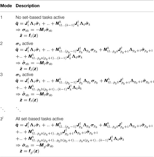
Table 2. System equations for the resulting 2^j modes for j low-priority set-based tasks.

For example, for a system with j = 3 set-based tasks and k = 6 equality tasks, p_a = 3 and p_b = p_c = 5, the 2^j = 8th mode would be

$\begin{array}{llll}\hfill \dot{\mathit{\text{q}}}& ={\mathit{\text{J}}}_1^{†}{\Lambda }_1{\tilde{\mathrm{\sigma }}}_1+{\mathit{\text{N}}}_1{\mathit{\text{J}}}_2^{†}{\Lambda }_2{\tilde{\mathrm{\sigma }}}_2+{\mathit{\text{N}}}_{12}^{\text{A}}{\mathit{\text{J}}}_3^{†}{\Lambda }_3{\tilde{\mathrm{\sigma }}}_3& \hfill & \\ \hfill & +{\mathit{\text{N}}}_{123\text{a}}^{\text{A}}{\mathit{\text{J}}}_4^{†}{\Lambda }_4{\tilde{\mathrm{\sigma }}}_4+{\mathit{\text{N}}}_{123\text{a}4}^{\text{A}}{\mathit{\text{J}}}_5^{†}{\Lambda }_5{\tilde{\mathrm{\sigma }}}_5+{\mathit{\text{N}}}_{123\text{a}45\text{bc}}^{\text{A}}{\mathit{\text{J}}}_6^{†}{\Lambda }_6{\tilde{\mathrm{\sigma }}}_6\end{array}$ (66)

All matrices M_i in Table 2 for i ∈ {1, … 2^j} are either equal to or a principal submatrix of the general matrix M in equation (60) in Antonelli (2009). Consequently, given Assumption 1, the matrices M_i are positive definite.

Consider the sets C₁-C_j defined by equations (29) and (30) with corresponding extended tangent cones as defined in equation (25). If the ith set-based task is inactive in a given mode f, the corresponding (n + i)th element of vector field f (x) must be in $T_{\mathbb{R},C_i}\left(\mathit{\text{x}}\right)$ for all x near z. If the same task is active, there is no requirement to the same element of the vector field. In mode 1, all the set-based tasks are inactive, thus all the (n + 1) to (n + j) elements of f₁(z) must be in their respective extended tangent cones for this mode to be chosen. In mode 2, only σ_a is active, so in this case all the (n + 2) to (n + j) elements of f₂(z) must be in their respective extended tangent cones if mode 2 should be the active mode. Thus, we define

$\begin{array}{llll}\hfill S_1& :=\left\{\mathit{\text{z}}\in {\mathbb{R}}^l:\exists \text{a\hspace{0.17em}neighborhood\hspace{0.17em}U\hspace{0.17em}of\hspace{0.17em}}\mathit{\text{z}}:\right.& \hfill & \\ \hfill & {\mathit{\text{f}}}_1\left(\mathit{\text{x}}\right)\in \left\{{\mathbb{R}}^n\times T_{\mathbb{R},C_1}\left(\mathit{\text{x}}\right)\right.\left.\left.\times \dots \times T_{\mathbb{R},C_j}\left(\mathit{\text{x}}\right)\times {\mathbb{R}}^{l-n-j}\right\}\forall \mathit{\text{x}}\in U\right\}\end{array}$ (67)

$\begin{array}{llll}\hfill S_2& :=\left\{\mathit{\text{z}}\in {\mathbb{R}}^l\setminus S_1:\exists \text{a\hspace{0.17em}nbhd\hspace{0.17em}U\hspace{0.17em}of\hspace{0.17em}}\mathit{\text{z}}:\right.& \hfill & \\ \hfill & f_2\left(\mathit{\text{x}}\right)\in \left\{{\mathbb{R}}^n\times \mathbb{R}\times T_{\mathbb{R},C_2}\left(\mathit{\text{x}}\right)\right.\left.\left.\times \dots \times T_{\mathbb{R},C_j}\left(\mathit{\text{x}}\right)\times {\mathbb{R}}^{l-n-j}\right\}\forall \mathit{\text{x}}\in U\right\}\end{array}$ (68)

$\begin{array}{llll}\hfill S_3& :=\left\{\mathit{\text{z}}\in {\mathbb{R}}^l\setminus \left(S_1\cup S_2\right):\exists \text{a\hspace{0.17em}nbhd\hspace{0.17em}U\hspace{0.17em}of\hspace{0.17em}}\mathit{\text{z}}:\right.& \hfill & \\ \hfill & f_3\left(\mathit{\text{x}}\right)\in \left\{{\mathbb{R}}^n\times T_{\mathbb{R},C_1}\left(\mathit{\text{x}}\right)\times \mathbb{R}\times T_{\mathbb{R},C_3}\right.\left.\left.\times \dots \times T_{\mathbb{R},C_j}\left(\mathit{\text{x}}\right)\times {\mathbb{R}}^{l-n-j}\right\}\forall \mathit{\text{x}}\in U\right\}\\ & :\end{array}$ (69)

$\begin{array}{ll}\hfill S_{2^j}& :=C\setminus \left(S_1\cup S_2\cup S_3\cup \dots \cup S_{2^j-1}\right).\end{array}$ (70)

The discontinuous equation $\dot{\mathit{\text{z}}}=\mathit{\text{f}}\left(\mathit{\text{z}}\right)$ with f : C → ℝ_l defined as

$\mathit{\text{f}}\left(\mathit{\text{z}}\right):=\left\{\begin{array}{cc}{\mathit{\text{f}}}_1\left(\mathit{\text{z}}\right)\hfill & \mathit{\text{z}}\in S_1\hfill \\ {\mathit{\text{f}}}_2\left(\mathit{\text{z}}\right)\hfill & \mathit{\text{z}}\in S_2\hfill \\ {\mathit{\text{f}}}_3\left(\mathit{\text{z}}\right)\hfill & \mathit{\text{z}}\in S_3\hfill \\ :\hfill & :\hfill \\ {\mathit{\text{f}}}_{2^j}\left(\mathit{\text{z}}\right)\hfill & \mathit{\text{z}}\in S_{2^j}\hfill \end{array}\right.$ (71)

then defines our system.

4.3. Combination of High- and Low-Priority Set-Based Tasks

Consider an n DOF robotic system with k equality tasks of m_i DOFs for i ∈ {1, …, k} and j set-based tasks ∈ ℝ, where j_x ≤ j of them are high priority and j − j_x are low-priority at any given priority level. Denote that the j_x th, (j_x + 1)th, and jth set-based task as σ_x, σ_y, and σ_z, respectively, where σ_x is the last high-priority set-based task, σ_y is the first low-priority set-based task, and σ_z is the lowest priority set-based task [x, y, and z represent the j_xth, (j_x + 1)th, and jth letter of the alphabet, respectively]. Consider the state-vector z ∈ ℝ^l, where

$l=n+j+{\displaystyle \sum _{i=1}^k}{m}_i,$ (72)

and

$\mathit{\text{z}}=\left[\begin{array}{c}\hfill \mathit{\text{q}}\hfill \\ \hfill {\mathrm{\sigma }}_{\text{sb}}\hfill \\ \hfill {\tilde{\mathrm{\sigma }}}_{\text{eb}}\hfill \end{array}\right]={\left[q_1,..,q_n,{\mathrm{\sigma }}_{\text{a}},..,{\mathrm{\sigma }}_{\text{x}},{\mathrm{\sigma }}_{\text{y}},..,{\mathrm{\sigma }}_{\text{z}},{\tilde{\mathrm{\sigma }}}_1^T,..,{\tilde{\mathrm{\sigma }}}_k^T\right]}_{.}^T$ (73)

It can be shown that the 2^j resulting modes from all possible combinations of active and inactive set-based tasks will reduce the error dynamics of the equality tasks to the form

${\dot{\tilde{\mathrm{\sigma }}}}_{\text{eb}}=-{\mathit{\text{M}}}_i{\tilde{\mathrm{\sigma }}}_{\text{eb}}$ (74)

for i = {1, …, 2^j}. The analysis is similar to the above sections and all matrices M_i are either equal to or a principal submatrix of the general matrix M in equation (60) in Antonelli (2009). Therefore, by Assumption 1, the matrices M_i are positive definite. Furthermore, as described in detail in Section 4.1, all the active high-priority set-based tasks are frozen in all modes.

Consider the sets

$\begin{array}{ll}\hfill C_1& :=\left[{\mathrm{\sigma }}_{\text{a,min}},{\mathrm{\sigma }}_{\text{a,max}}\right],\\ :\end{array}$ (75)

$\begin{array}{lll}\hfill & \hfill & \\ \hfill C_{j_x}& :=\left[{\mathrm{\sigma }}_{\text{x,min}},{\mathrm{\sigma }}_{\text{x,max}}\right],\end{array}$ (76)

$\begin{array}{ll}\hfill C_{j_x+1}& :=\left[{\mathrm{\sigma }}_{\text{y,min}},{\mathrm{\sigma }}_{\text{y,max}}\right],\\ \hfill & :\end{array}$ (77)

$\begin{array}{ll}\hfill C_j& :=\left[{\mathrm{\sigma }}_{\text{z,min}},{\mathrm{\sigma }}_{\text{z,max}}\right],\end{array}$ (78)

$\begin{array}{ll}\hfill C& :={\mathbb{R}}^n\times C_1\times \dots \times C_{j_x}\times {\mathbb{R}}^{j-j_x}\times {\mathbb{R}}^{l-n-j}\end{array}$ (79)

and

$\begin{array}{ll}\hfill T_{C_1}\left(\mathit{\text{z}}\right)& =\left\{\begin{array}{cc}\left[0,\infty \right)\hfill & {\mathrm{\sigma }}_{\text{a}}={\mathrm{\sigma }}_{\text{a},\text{min}}\hfill \\ \mathbb{R}\hfill & {\mathrm{\sigma }}_{\text{a}}\in \left({\mathrm{\sigma }}_{\text{a},\text{min}},{\mathrm{\sigma }}_{\text{a},\text{max}}\right)\hfill \\ \left(-\infty ,0\right]\hfill & {\mathrm{\sigma }}_{\text{a}}={\mathrm{\sigma }}_{\text{a},\text{max}}\hfill \end{array}\right.,\hfill \\ \hfill & :\end{array}$ (80)

$\begin{array}{ll}\hfill T_{C_{j_x}}\left(\mathit{\text{z}}\right)& =\left\{\begin{array}{cc}\left[0,\infty \right)\hfill & {\mathrm{\sigma }}_{\text{x}}={\mathrm{\sigma }}_{\text{x,min}}\hfill \\ \mathbb{R}\hfill & {\mathrm{\sigma }}_{\text{x}}\in \left({\mathrm{\sigma }}_{\text{x,min}},{\mathrm{\sigma }}_{\text{x,max}}\right)\hfill \\ \left(-\infty ,0\right]\hfill & {\mathrm{\sigma }}_{\text{x}}={\mathrm{\sigma }}_{\text{j,max}}\hfill \end{array}\right.\hfill \end{array}$ (81)

$\begin{array}{ll}\hfill T_{\mathbb{R},C_{j_x+1}}\left(\mathit{\text{z}}\right)& =\left\{\begin{array}{cc}\left[0,\infty \right)\hfill & {\mathrm{\sigma }}_{\text{y}}\le {\mathrm{\sigma }}_{\text{y,min}}\hfill \\ \mathbb{R}\hfill & {\mathrm{\sigma }}_{\text{y}}\in \left({\mathrm{\sigma }}_{\text{y,min}},{\mathrm{\sigma }}_{\text{y,max}}\right)\hfill \\ \left(-\infty ,0\right]\hfill & {\mathrm{\sigma }}_{\text{y}}\ge {\mathrm{\sigma }}_{\text{y,max}}\hfill \end{array}\right.\hfill \\ \hfill & :\hfill \end{array}$ (82)

$\begin{array}{ll}\hfill T_{\mathbb{R},C_j}\left(\mathit{\text{z}}\right)& =\left\{\begin{array}{cc}\left[0,\infty \right)\hfill & {\mathrm{\sigma }}_{\text{z}}\le {\mathrm{\sigma }}_{\text{z,min}}\hfill \\ \mathbb{R}\hfill & {\mathrm{\sigma }}_{\text{z}}\in \left({\mathrm{\sigma }}_{\text{z,min}},{\mathrm{\sigma }}_{\text{z,max}}\right)\hfill \\ \left(-\infty ,0\right]\hfill & {\mathrm{\sigma }}_{\text{z}}\ge {\mathrm{\sigma }}_{\text{z,max}}\hfill \end{array}\right..\hfill \end{array}$ (83)

$\begin{array}{ll}\hfill {\mathit{\text{T}}}_{C_{\text{h}}}\left(\mathit{\text{z}}\right)& =T_{C_1}\left(\mathit{\text{z}}\right)\times T_{C_2}\left(\mathit{\text{z}}\right)\times \dots \times T_{C_{j_x}}\left(\mathit{\text{z}}\right)\end{array}$ (84)

$\begin{array}{ll}\hfill {\mathit{\text{T}}}_C\left(\mathit{\text{z}}\right)& ={\mathbb{R}}^n\times {\mathit{\text{T}}}_{C_{\text{h}}}\left(\mathit{\text{z}}\right)\times {\mathbb{R}}^{j-j_x}\times {\mathbb{R}}^{l-n-j}.\end{array}$ (85)

Note that z ∈ C only implies that all the high-priority set-based tasks are within their respective desired sets. Furthermore, the tangent cones are considered for the high-priority set-based tasks, and the extended tangent cones for the low-priority ones.

$\begin{array}{ll}\hfill & S_1:=\{\mathit{\text{z}}\in C:\exists \text{a}\text{neighborhood}\text{U}\text{of}\mathit{\text{z}}:\end{array}$ (86)

$\begin{array}{llll}\hfill & {\mathit{\text{f}}}_1\left(\mathit{\text{x}}\right)\in \left\{\underset{\triangleq {\mathit{\text{T}}}_{C_{\text{qh}}}\left(\mathit{\text{x}}\right)}{\underbrace{{\mathbb{R}}^n\times {\mathit{\text{T}}}_{C_{\text{h}}}\left(\mathit{\text{x}}\right)}}\times T_{\mathbb{R},C_{j_{\mathit{\text{x}}}+1}}\left(\mathit{\text{x}}\right)\right.\left.\left.\times \dots \times \underset{\triangleq T_{\mathbb{R},C_{j\mathrm{\sigma }}\left(\mathit{\text{x}}\right)}}{\underbrace{{\mathit{\text{T}}}_{\mathbb{R},C_j}\left(\mathit{\text{x}}\right)\times {\mathbb{R}}^{l-n-j}}}\right\}\forall \mathit{\text{x}}\in C\cap U\right\}& \hfill & \\ \hfill & S_2:=\{\mathit{\text{z}}\in C:\setminus S_1:\exists \text{a}\text{nbhd}\text{U}\text{of}\mathit{\text{z}}:\end{array}$ (87)

$\begin{array}{llll}\hfill & \left.{\mathit{\text{f}}}_2\left(\mathit{\text{x}}\right)\in \left\{{\mathit{\text{T}}}_{C_{\text{qh}}}\left(\mathit{\text{x}}\right)\times T_{\mathbb{R},C_{j_x+1}}\left(\mathit{\text{x}}\right)\times \dots \times {\mathit{\text{T}}}_{\mathbb{R},C_{j\mathrm{\sigma }}}\left(\mathit{\text{x}}\right)\right\}\forall \mathit{\text{x}}\in C\cap U\right\}& \hfill & \\ \hfill & :& \hfill & \\ \hfill & S_{j_x+1}:=\left\{\mathit{\text{z}}\in C\setminus \left(S_1\cup \dots \cup S_{j_x}\right):\exists \text{a}\text{nbhd}\text{U}\text{of}\mathit{\text{z}}:\right.\end{array}$ (88)

$\begin{array}{llll}\hfill & {\mathit{\text{f}}}_{j_x+1}\left(\mathit{\text{x}}\right)\in \left\{{\mathit{\text{T}}}_{C_{\text{qh}}}\left(\mathit{\text{x}}\right)\times T_{\mathbb{R},C_{j_x+1}}\left(\mathit{\text{x}}\right)\right.\left.\left.\times \dots \times {\mathit{\text{T}}}_{\mathbb{R},C_{j\mathrm{\sigma }}}\left(\mathit{\text{x}}\right)\right\}\forall \mathit{\text{x}}\in C\cap U\right\}& \hfill & \\ \hfill & S_{j_x+2}:=\left\{\mathit{\text{z}}\in C\setminus \left(S_1\cup \dots \cup S_{j_x+1}\right):\exists \text{a}\text{nbhd}\text{U}\text{of}\mathit{\text{z}}:\right.\end{array}$ (89)

$\begin{array}{llll}\hfill & {\mathit{\text{f}}}_{j_x+2}\left(\mathit{\text{x}}\right)\in \left\{{\mathit{\text{T}}}_{C_{\text{qh}}}\left(\mathit{\text{x}}\right)\times \mathbb{R}\times T_{\mathbb{R},C_{j_x+2}}\left(\mathit{\text{x}}\right)\right.\left.\left.\times \dots \times {\mathit{\text{T}}}_{\mathbb{R},C_{j\mathrm{\sigma }}}\left(\mathit{\text{x}}\right)\right\}\forall \mathit{\text{x}}\in C\cap U\right\}& \hfill & \\ \hfill & S_{j_x+3}:=\left\{\mathit{\text{z}}\in C\setminus \left(S_1\cup \dots \cup S_{j_x+2}\right):\exists \text{a}\text{nbhd}\text{U}\text{of}\mathit{\text{z}}:\right.\end{array}$ (90)

$\begin{array}{llll}\hfill & {\mathit{\text{f}}}_{j_x+3}\left(\mathit{\text{x}}\right)\in \left\{{\mathit{\text{T}}}_{C_{\text{qh}}}\left(\mathit{\text{x}}\right)\times T_{\mathbb{R},C_{j_x+1}}\left(\mathit{\text{x}}\right)\times \mathbb{R}\times T_{\mathbb{R},C_{j_x+3}}\left(\mathit{\text{x}}\right)\right.\left.\times \dots \times {\mathit{\text{T}}}_{\mathbb{R},C_{j\mathrm{\sigma }}}\left(\mathit{\text{x}}\right)\forall \mathit{\text{x}}\in C\cap U\right\}& \hfill & \\ \hfill & :& \hfill & \\ \hfill & S_{2^j}:=C\setminus \left(S_1\cup S_2\cup S_3\cup \dots \cup S_{2^j-1}\right).\end{array}$ (91)

The discontinuous equation $\dot{\mathit{\text{z}}}=\mathit{\text{f}}\left(\mathit{\text{z}}\right)$ with f : C → ℝ^l defined as

$\mathit{\text{f}}\left(\mathit{\text{z}}\right):=\left\{\begin{array}{cc}{\mathit{\text{f}}}_1\left(\mathit{\text{z}}\right)\hfill & \mathit{\text{z}}\in S_1\hfill \\ {\mathit{\text{f}}}_2\left(\mathit{\text{z}}\right)\hfill & \mathit{\text{z}}\in S_2\hfill \\ {\mathit{\text{f}}}_3\left(\mathit{\text{z}}\right)\hfill & \mathit{\text{z}}\in S_3\hfill \\ :\hfill & :\hfill \\ {\mathit{\text{f}}}_{2^j}\left(\mathit{\text{z}}\right)\hfill & \mathit{\text{z}}\in S_{2^j}\hfill \end{array}\right.$ (92)

then defines our system. Similar to the analysis of the previous sections, in the sets S_i, i ∈ {1, …, 2^j}, the elements of the vector flows f_i(z) corresponding to the high-priority set-based tasks are required to be in their respective tangent cone in all modes, and the elements corresponding to the low-priority set-based tasks are required to be in the corresponding extended tangent cone only in the modes where that task is inactive.

5. Stability Analysis

To study the behavior of the discontinuous differential equations [equation (92)], we look at the corresponding constrained differential inclusion:

$\mathit{\text{z}}\in C\dot{\mathit{\text{z}}}\in \mathit{\text{F}}\left(\mathit{\text{z}}\right)$ (93)

where

$\mathit{\text{F}}\left(\mathit{\text{z}}\right):={\displaystyle \bigcap _{\mathrm{\delta }>0}}\text{co}\overline{\mathit{\text{f}}\left(\left(z+\mathrm{\delta }\mathbb{B}\right)\cap C\right)}\forall \mathit{\text{z}}\in C.$ (94)

𝔹 is a unit ball in ℝ^dim(z) centered at the origin. $\text{co}\overline{P}$ denotes the closed convex hull of the set P, or in other words, the smallest closed convex set containing P. The state evolution of z is the Krasovskii solution of the discontinuous differential equation (55) [Definition 4.2 (Goebel et al., 2012)].

5.1. Convergence of Equality Tasks

The first part of the stability proof considers the convergence of the system equality tasks when switching between 2^j possible modes of the system.

If V is a continuously differentiable Lyapunov function for $\dot{\mathit{\text{z}}}={\mathit{\text{f}}}_i\left(\mathit{\text{z}}\right)$ for all i ∈ {1, …, 2^j}, then V is a Lyapunov function for $\dot{\mathit{\text{z}}}\in \mathit{\text{F}}\left(\mathit{\text{z}}\right)$. The following equation holds as all f_i(z) are continuous functions:

$\mathit{\text{f}}\in \mathit{\text{F}}\left(\mathit{\text{z}}\right)\Rightarrow \mathit{\text{f}}={\mathrm{\lambda }}_1{\mathit{\text{f}}}_1\left(\mathit{\text{z}}\right)+{\mathrm{\lambda }}_2{\mathit{\text{f}}}_2\left(\mathit{\text{z}}\right)+\dots +{\mathrm{\lambda }}_{2^j}{\mathit{\text{f}}}_{2^j}\left(\mathit{\text{z}}\right)$ (95)

for some ${\displaystyle \sum _{i=1}^{2^j}}{\mathrm{\lambda }}_i=1,{\mathrm{\lambda }}_i\ge 0.$ Consider the Lyapunov function candidate for the equality task errors:

$V\left({\tilde{\mathrm{\sigma }}}_{{}_{\text{eb}}}\right)=\frac{1}{2}{\tilde{\mathrm{\sigma }}}_{{}_{\text{eb}}}^T{\tilde{\mathrm{\sigma }}}_{{}_{\text{eb}}}.$ (96)

Using equation (95) and the system equations given in Tables 1 and 2 for high-priority and low-priority set-based tasks, respectively, we find that the time derivative of V is given by

$\begin{array}{ll}\hfill \begin{array}{rl}\dot{V}& ={\tilde{\mathrm{\sigma }}}_{{}_{\text{eb}}}^T\left({\mathrm{\lambda }}_1\left(-{\mathit{\text{M}}}_1{\tilde{\mathrm{\sigma }}}_{{}_{\text{eb}}}\right)+{\mathrm{\lambda }}_2\left(-{\mathit{\text{M}}}_2{\tilde{\mathrm{\sigma }}}_{{}_{\text{eb}}}\right)+\dots +{\mathrm{\lambda }}_{2^j}\left(-{\mathit{\text{M}}}_{2^j}{\tilde{\mathrm{\sigma }}}_{{}_{\text{eb}}}\right)\right)\\ & =-{\tilde{\mathrm{\sigma }}}_{{}_{\text{eb}}}^T\left({\mathrm{\lambda }}_1{\mathit{\text{M}}}_1+{\mathrm{\lambda }}_2{\mathit{\text{M}}}_2+\dots +{\mathrm{\lambda }}_{2^j}{\mathit{\text{M}}}_{2^j}\right){\tilde{\mathrm{\sigma }}}_{{}_{\text{eb}}}\\ & =-{\tilde{\mathrm{\sigma }}}_{{}_{\text{eb}}}^T\mathit{\text{Q}}{\tilde{\mathrm{\sigma }}}_{{}_{\text{eb}}}.\end{array}& \end{array}$ (97)

The convex combination Q of positive-definite matrices is also positive definite. Therefore, $\dot{V}$ is negative definite and ${\tilde{\mathrm{\sigma }}}_{{}_{\text{eb}}}=\mathbf{\text{0}}$ is a globally asymptotically stable equilibrium point in all modes. Thus, the equality task errors ${\tilde{\mathrm{\sigma }}}_{{}_{\text{eb}}}$ asymptotically converge to zero when switching between modes. Furthermore, if q belongs to a compact set, the equilibrium point ${\tilde{\mathrm{\sigma }}}_{\text{eb}}=\mathbf{\text{0}}$ is exponentially stable.

5.2. Satisfaction of Set-Based Tasks and Existence of Solution

The second part of the stability proof considers the satisfaction of the set-based tasks and the existence of a valid solution.

The analysis made in Section 4.2.1 concluded that the evolution of active low-priority set-based tasks is influenced by the higher-priority equality tasks. Unlike the high-priority set-based tasks they cannot be frozen at any given time, and therefore they cannot be guaranteed to be satisfied. We have defined a closed set C in equation (79) within which all high-priority set-based tasks are satisfied at all times. As long as the system solution z ∈ C, these tasks are not violated.

For a system described by equation (92), $\dot{\mathit{\text{z}}}={\mathit{\text{f}}}_1\left(\mathit{\text{z}}\right)$ as long as the solution z ∈ C and the lower-priority set-based tasks outside of their respective desired sets do not move further away from them. If the system reaches the boundary of C and remaining in mode 1 would cause z to leave C, another mode is activated. If neither of the vector fields ${\mathit{\text{f}}}_1-{\mathit{\text{f}}}_{2^j-1}$ will result in z staying in C, the chosen solution is $\dot{\mathit{\text{z}}}={\mathit{\text{f}}}_{2^j}\left(\mathit{\text{z}}\right)$, for which it has been shown that ${\dot{\mathrm{\sigma }}}_{\text{a}}$ to ${\dot{\mathrm{\sigma }}}_{\text{x}}\equiv 0$. Therefore, ${\mathit{\text{f}}}_{2^j}\left(\mathit{\text{z}}\right)\in {\mathit{\text{T}}}_C\left(\mathit{\text{z}}\right)\forall \mathit{\text{z}}\in C$, and C is strongly forward invariant for $\dot{\mathit{\text{z}}}={\mathit{\text{f}}}_{2^j}\left(\mathit{\text{z}}\right)$. Thus, there will always exist a solution z ∈ C and the high-priority set-based tasks are consequently always satisfied.

6. Implementation

This section presents the practical implementation of the proposed algorithm and discusses the computational load of running it.

In the stability analysis, only regulation equality tasks are considered, that is tasks with ${\dot{\mathrm{\sigma }}}_{\text{des}}\equiv \mathbf{\text{0}}$. For practical purposes, one can also apply this algorithm for time-varying equality tasks as in equation (21). An example of this is presented in Section 7. Furthermore, for the stability analysis, the lower-priority set-based tasks are handled the same way as the high-priority ones and are attempted frozen. However, as this can not be guaranteed, they might exceed their desired set. With this in mind, for practical purposes, these tasks can be handled by defining σ_des = σ_max and σ_des = σ_min if σ ≥ σ_max and ≤σ_min, respectively. Should σ leave the set, the solution will actively attempt to bring σ back to the border of its valid set (rather than simply freezing it outside the set) by having a non-zero error feedback σ as it does in, for instance, equation (56).

In the implementation, the Boolean function in_T_RC defined in Algorithm 1 is used to check if the time-derivative of a set-based task σ with a valid set C = [σ_min, σ_max] is in the modified tangent cone of C, i.e., if $\dot{\mathrm{\sigma }}\in T_{\mathbb{R},C}\left(\mathrm{\sigma }\right)$. The algorithm in_T_RC is illustrated in Figure 2.

ALGORITHM 1

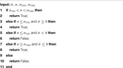
Algorithm 1. The Boolean function in_T_RC.

FIGURE 2

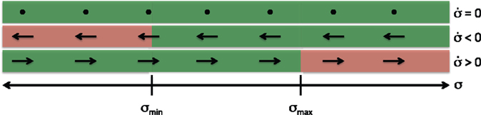
Figure 2. Graphic illustration of the function in_T_RC with return value True shown in green and False in red. The function only returns False when σ is outside or on the border of its valid set and the derivative points away from the valid set.

Note that in the implementation of the algorithm, in_T_RC is used as a check both for the high-priority and low-priority set-based task. This is to handle small numerical inaccuracies that result from discretization of a continuous system. Furthermore, given initial conditions outside the valid set C, the chosen implementation is still well-defined for all set-based tasks.

For a system with j set-based tasks, the 2^j modes must be calculated every time step. For practical purposes, it is only necessary to calculate the part of the state vector z that corresponds to q, so we calculate this using $\dot{\mathit{\text{q}}}={\mathit{\text{f}}}_i\left(\mathit{\text{q}}\right)$ for i ∈ {1, …, 2^j}. Then, to decide what mode to activate, in_T_RC is used to check if every inactive set-based task of that mode returns True. If it does, that mode is picked. If not, the next mode is considered. Recall that ${\dot{\mathrm{\sigma }}}_{\text{k}}={\mathit{\text{J}}}_{\text{k}}\dot{\mathit{\text{q}}}$ and denote the jth set-based task as σ_z. Define the Boolean variables ϕ_i

$\begin{array}{l}{\mathit{\varphi }}_i\text{\hspace{0.17em}≜\hspace{0.17em}in\_T\_RC}\left({\mathit{\text{J}}}_{\mathit{\varphi }}{\mathit{\text{f}}}_i,{\mathrm{\sigma }}_{\mathit{\varphi }},{\mathrm{\sigma }}_{\mathit{\varphi },\text{min}},{\mathrm{\sigma }}_{\mathit{\varphi },\text{max}}\right)\hfill \\ \text{for\hspace{0.17em}}i\in \left\{1,\dots ,2^j\right\}\text{\hspace{0.17em}and\hspace{0.17em}}\mathit{\varphi }\text{\hspace{0.17em}in\hspace{0.17em}}\left\{\text{a},\dots ,\text{z}\right\}\end{array}$ (98)

The active mode is chosen according to Table 3, where the algorithm iterates through priority 1 to 2^j and activates the first mode that satisfies the criteria presented in Table 3. The modes are assigned priority according to their restrictiveness. The more set-based tasks are active, the more restrictive it is. Therefore, the least restrictive mode is f₁, where no set-based tasks are active. From there, f₂ − f_(j+1) are the modes where one set-based task is active, etc. In Table 3, a hyphen indicates that the Boolean value does not need to be checked because in that mode, the corresponding set-based task is active and therefore satisfied by definition (in case of a high-priority set-based task) or actively handled to the best of the system’s ability (in case of a low-priority set-based task).

TABLE 3

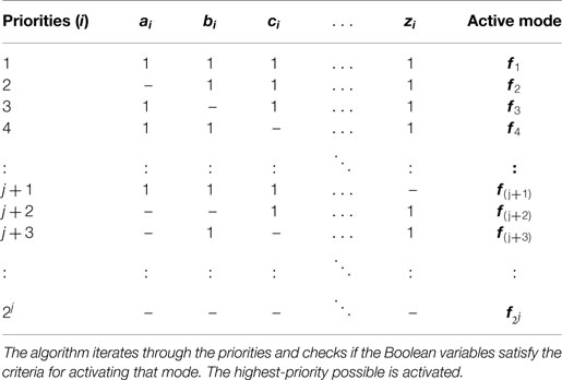
Table 3. Table illustrating the activation of mode based on the Boolean variables as defined in equation (98).

6.1. Computational Load

Differently from Escande et al. (2014), the proposed algorithm is deterministic from the computational load aspect. It is possible, in fact, to provide an estimate with respect to the main parameters of the system. In particular, it is seen that the most critical variable for the computational load is the number of DOFs of the system.

The cost of a certain operation is denoted as c(⋅), the following assumptions have been done:

• sum and subtraction have zero cost,

• the cost of matrix multiplication between a m× p and a p × n is proportional to mpn,

• the cost of matrix inversion of a n × n is proportional to n³.

Denoting the number of DOFs of the system as n and the generic task dimension as m_x, the following holds:

$\begin{array}{l}\hfill c\left({\mathit{\text{J}}}_{\text{x}}^{†}\right)={\mathrm{\alpha }}_{1}n{m}_{\text{x}}^2+{\mathrm{\alpha }}_2{m}_{\text{x}}^3\end{array}$ (99)

$\begin{array}{l}\hfill c\left({\mathit{\text{N}}}_{\text{x}}\right)={\mathrm{\alpha }}_{1}n{m}_{\text{x}}^2+{\mathrm{\alpha }}_2{m}_{\text{x}}^3+{\mathrm{\alpha }}_3{n}^2{m}_{\text{x}}\end{array}$ (100)

$\begin{array}{l}\hfill c\left({\dot{\mathit{\text{q}}}}_{\text{x}}\right)={\mathrm{\alpha }}_{1}n{m}_{\text{x}}^2+{\mathrm{\alpha }}_2{m}_{\text{x}}^3+{\mathrm{\alpha }}_4{\text{nm}}_{\text{x}}\end{array}$ (101)

By considering two generic a and b tasks, each projection within the null-space costs:

$\begin{array}{llll}\hfill c\left({\mathit{\text{N}}}_{\text{a}}{\dot{\mathit{\text{q}}}}_{\text{b}}\right)& ={\mathrm{\alpha }}_{1}n{m}_{\text{a}}^2+{\mathrm{\alpha }}_2{m}_{\text{a}}^3+{\mathrm{\alpha }}_3{n}^2{m}_{\text{a}}+& \hfill & \\ \hfill & +{\mathrm{\alpha }}_{1}n{m}_{\text{b}}^2+{\mathrm{\alpha }}_2{m}_{\text{b}}^3+{\mathrm{\alpha }}_{4}n{m}_{\text{b}}+{\mathrm{\alpha }}_5{n}^2.\end{array}$ (102)

In the proposed method, this computational cost is present as many times as there are equality plus active set-based tasks. However, it is easy to recognize that this cost is small for the higher-priority task and grows when the lowest priority are projected into the null space of the stacked Jacobian of all the higher priorities. The worst case, from the computational aspect, arises thus when m_a or m_b are as large as possible, i.e., n − 1, in which case

$c\left({\mathit{\text{N}}}_{\text{a}}{\dot{\mathit{\text{q}}}}_{\text{b}}\right)\propto n^3.$ (103)

By assuming that all the DOFs are exploited, it is possible to verify that this cost arises both in the classical equality-task-priority inverse kinematics and in the extension to set-based tasks presented here.

The recursive computation of the null spaces given in Antonelli et al. (2015) does not change the dependence of the cost with respect to the number of DOFs of the system, since it implies a matrix multiplication between two n × n matrices whose cost still is proportional to n³.

Overall, the cost is proportional to n³.

One additional computation cost arising for the set-based extension in this paper is the check whether or not one of the possible solutions is violating one of the set-based tasks. This implies re-projection of ${\dot{\mathit{\text{q}}}}_{\text{des}}$ by means of J_x at an individual cost of nm_x. However, we only consider scalar set-based tasks, for which m_x = 1 and the cost is proportional to n.

Furthermore, for j set-based tasks, in the worst-case scenario, it is necessary to compute 2^j possible solutions. However, in many cases, some of the 2^j modes have common terms, which will reduce the overall cost, since these terms only need to be computed once. Furthermore, simulations and experimental results confirm that the algorithm is feasible and sufficiently fast for real-time applications.

It is also worth noticing that optimized algorithms for matrix inversion exist but are not considered here. In fact, optimized methods usually exhibit different performances based on the input, and in general, they have a smaller cost than the costs considered here.

7. Experimental Results

This section presents experimental results that were obtained by running the proposed algorithm on a 6 DOF manipulator from Universal Robots called UR5. Two examples are presented that illustrate the implementation and effectiveness of the proposed method.

7.1. UR5 and Control Setup

The UR5 is a manipulator with 6 revolute joints, and the joint angles are denoted $\mathit{\text{q}}\triangleq {\left[\begin{array}{cccccc}\hfill q_1\hfill & \hfill q_2\hfill & \hfill q_3\hfill & \hfill q_4\hfill & \hfill q_5\hfill & \hfill q_6\hfill \end{array}\right]}^{\text{T}}$. In this paper, the Denavit–Hartenberg (D–H) parameters are used to calculate the forward kinematics. The parameters are given in Wu et al. (2014) and are presented Table 4 with the corresponding coordinate frames illustrated in Figure 3. The resulting forward kinematics has been experimentally verified to confirm the correctness of the parameters.

TABLE 4

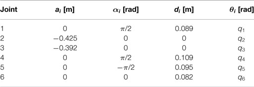
Table 4. Table of the D–H parameters of the UR5.

FIGURE 3

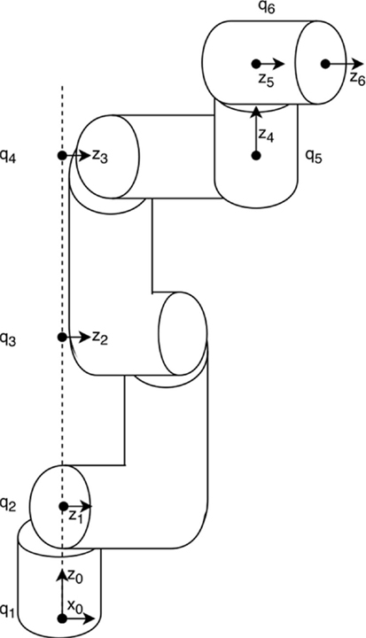
Figure 3. Coordinate frames corresponding to the D–H parameters in Table 4.

The UR5 is equipped with a high-level controller that can control the robot both in joint and Cartesian space. In the experiments presented here, a calculated reference q_des is sent to the high-level controller, which is assumed to function nominally such that

$\mathit{\text{q}}\approx {\mathit{\text{q}}}_{\text{des}}.$ (104)

From this reference, ${\dot{\mathit{\text{q}}}}_{\text{des}}$ and ${\ddot{\mathit{\text{q}}}}_{\text{des}}$ are extrapolated and sent with q_des to the low-level controller.

The structure of the system is illustrated in Figure 4. The algorithm described in Section 6 is implemented in the kinematic controller block. For every time step, a reference for the joint velocities is calculated and integrated to desired joint angles q_des. This is used as input to the dynamic controller, which in turn applies torques to the joint motors. Note that the actual state q is not used for feedback to the kinematic control block. When the current state is used as input for the kinematic controller, the kinematic and dynamic loops are coupled and the gains designed for the kinematic control alone to satisfy Assumption 1 can not be used. This result in uneven motion, and therefore the kinematic control block receives the previous reference as feedback, which leads to much nicer behavior, and is a good approximation because the dynamic controller tracks the reference with very high precision. This is a standard method of implementation for industry robots when kinematic control is used.

FIGURE 4

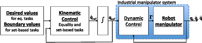
Figure 4. The control structure of the experiments. The tested algorithm is implemented in the kinematic controller block.

The communication between the implemented algorithm and the industrial manipulator system occurs through a TCP/IP connection, which operates at 125 Hz. The kinematic control block is implemented using python, which is a very suitable programing language for the task. The TCP/IP connection is very simple to set up in python. Furthermore, python has several libraries that can handle different math and matrix operations.

7.2. Implemented Tasks

Three tasks make up the basis for the experiments: position control, collision avoidance, and field of view (FOV). Position control is implemented as both an equality and set-based task and collision avoidance and FOV as set-based tasks.

7.2.1. Position Control

The position of the end-effector relative to the base coordinate frame is given by the forward kinematics. The analytical expression can be found through the homogeneous transformation matrix (Spong et al., 2005) using the D–H parameters given in Table 4. The task is then defined by

$\begin{array}{l}\hfill {\mathrm{\sigma }}_{\text{pos}}=\mathit{\text{f}}\left(\mathit{\text{q}}\right)\in {\mathbb{R}}^3\end{array}$ (105)

$\begin{array}{l}\hfill {\dot{\mathrm{\sigma }}}_{\text{pos}}={\mathit{\text{J}}}_{\text{pos}}\left(\mathit{\text{q}}\right)\dot{\mathit{\text{q}}}=\frac{\mathrm{d}\mathbf{f}}{\mathrm{d}\mathit{\text{q}}}\dot{\mathit{\text{q}}},\end{array}$ (106)

where the function f (q) is given by the forward kinematics.

7.2.2. Collision Avoidance

To avoid a collision between the end effector and an object at position p_o ∈ ℝ³, the distance between them is used as a task:

$\begin{array}{l}\hfill {\mathrm{\sigma }}_{\text{CA}}=\sqrt{{\left({\mathit{\text{p}}}_o-{\mathrm{\sigma }}_{\text{pos}}\right)}^{\text{T}}\left({\mathit{\text{p}}}_o-{\mathrm{\sigma }}_{\text{pos}}\right)}\in \mathbb{R}\end{array}$ (107)

$\begin{array}{l}\hfill {\dot{\mathrm{\sigma }}}_{\text{CA}}={\mathit{\text{J}}}_{\text{CA}}\left(\mathit{\text{q}}\right)\dot{\mathit{\text{q}}}=-\frac{{\left({\mathit{\text{p}}}_o-{\mathrm{\sigma }}_{\text{pos}}\right)}^{\text{T}}}{{\mathrm{\sigma }}_{\text{CA}}}{\mathit{\text{J}}}_{\text{pos}}\left(\mathit{\text{q}}\right)\dot{\mathit{\text{q}}}\end{array}$ (108)

7.2.3. Field of View

The field of view is defined as the outgoing vector of the end effector, i.e., the z₆-axis in Figure 3. This vector expressed in base coordinates is denoted a ∈ ℝ³ and can be found through the homogeneous transformation matrix using the D–H parameters:

$\begin{array}{l}\hfill \mathit{\text{a\hspace{0.17em}}}=\mathit{g}\left(\mathit{\text{q}}\right)\in {\mathbb{R}}^3\end{array}$ (109)

$\begin{array}{l}\hfill \dot{\mathit{\text{a}}}={\mathit{\text{J}}}_{\text{FOV},3\text{DOF}}\left(\mathit{\text{q}}\right)\dot{\mathit{\text{q}}}=\frac{\mathrm{d}\mathit{\text{g}}}{\mathrm{d}\mathit{\text{q}}}\dot{\mathit{\text{q}}}\end{array}$ (110)

FOV is a useful task when directional devices or sensors are mounted on the end effector, and they are desired to point in a certain direction a_des ∈ ℝ³. The task is defined as the norm of the error between a and a_des:

$\begin{array}{l}\hfill {\mathrm{\sigma }}_{\text{FOV}}=\sqrt{{\left({\mathit{\text{a}}}_{\text{des}}-\mathit{\text{a}}\right)}^{\text{T}}\left({\mathit{\text{a}}}_{\text{des}}-\mathit{\text{a}}\right)}\in \mathbb{R}\end{array}$ (111)

$\begin{array}{l}\hfill {\dot{\mathrm{\sigma }}}_{\text{FOV}}={\mathit{\text{J}}}_{\text{FOV}}\left(\mathit{\text{q}}\right)\dot{\mathit{\text{q}}}=-\frac{{\left({\mathit{\text{a}}}_{\text{des}}-\mathit{\text{a}}\right)}^{\text{T}}}{{\mathrm{\sigma }}_{\text{FOV}}}{\mathit{\text{J}}}_{\text{FOV},3\text{DOF}}\left(\mathit{\text{q}}\right)\dot{\mathit{\text{q}}}\end{array}$ (112)

Note in equations (108) and (112) that J_CA and J_FOV are not defined for σ_CA = 0 and σ_FOA = 0, respectively. In the implementation, this is solved by adding a small ε > 0 to the denominator of these two Jacobians, thereby ensuring that division by zero does not occur. Furthermore, the method presented in this paper ensures collision avoidance; hence, σ_CA will never be zero. Also, note that alternative FOV functions exist which do not suffer from this representation singularity.

7.3. Example 1

In this example, the system has been given two waypoints for the end effector to reach. This is the sole equality task σ₁ of this example:

$\begin{array}{l}{\mathit{\text{p}}}_{\text{w}1}={\left[0.486\text{\hspace{0.17em}m}-0.066\text{\hspace{0.17em}m}-0.250\text{\hspace{0.17em}m}\right]}^{\text{T}},\text{and}\end{array}$ (113)

$\begin{array}{l}{\mathit{\text{p}}}_{\text{w2}}={\left[0.320\text{\hspace{0.17em}m}0.370\text{\hspace{0.17em}m}-0.250\text{\hspace{0.17em}m}\right]}^{\text{T}}.\end{array}$ (114)

A circle of acceptance (COA) of 0.02 m is implemented for switching from σ_1,des = σ_pos,des = p_w1 to σ_1,des = σ_pos,des = p_w2. The task gain matrix has been chosen as

${\Lambda }_{\text{pos}}=\text{diag}\left(\left[\begin{array}{ccc}\hfill 0.3\hfill & \hfill 0.3\hfill & \hfill 0.3\hfill \end{array}\right]\right).$ (115)

Furthermore, two obstacles have been introduced; hence, two collision avoidance tasks are necessary. In this example, these tasks are high-priority and are denoted σ_a and σ_b, respectively. The obstacles are positioned at

$\begin{array}{l}\hfill {\mathit{\text{p}}}_{\text{o}1}={\left[0.40\text{\hspace{0.17em}m}-0.25\text{\hspace{0.17em}m}-0.33\text{\hspace{0.17em}m}\right]}^{\text{T}},\text{\hspace{0.17em}and}\end{array}$ (116)

$\begin{array}{l}\hfill {\mathit{\text{p}}}_{\text{o2}}={\left[0.40\text{\hspace{0.17em}m}0.15\text{\hspace{0.17em}m}-0.33\text{\hspace{0.17em}m}\right]}^{\text{T}},\end{array}$ (117)

and have a radius of 0.18 and 0.15 m, respectively. This radius is used as the minimum value of the set-based collision avoidance task to ensure that the end effector is never closer to the obstacle center than the allowed radius, see Table 5. Because the task is only considered as a high-priority set-based task, it is not necessary to choose a task gain.

TABLE 5

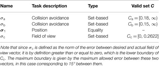
Table 5. Implemented tasks in example 1 sorted by decreasing priority.

FOV is implemented as a low-priority set-based task σ_c = σ_FOV, with a maximum value to limit the error between a and a_des. Here, the maximum value for the set-based FOV task is set as 0.2622. This corresponds to allowing the angle between a_des and a being 15° or less. If the FOV error exceeds, the maximum value of 0.2622, rather than attempting to freeze the task at its current value, an effort is made to push it back to the boundary of the valid set:

${\tilde{\mathrm{\sigma }}}_{\text{c}}={\mathrm{\sigma }}_{\text{FOV},\text{max}}-{\mathrm{\sigma }}_{\text{c}}=0.2622-{\mathrm{\sigma }}_{\text{FOV}}$ (118)

with

${\mathit{\text{a}}}_{\text{des}}\equiv {\left[\begin{array}{ccc}\hfill 1\hfill & \hfill 0\hfill & \hfill 0\hfill \end{array}\right]}^{\text{T}}.$ (119)

The gain for this task is Λ_FOV = 1. The priority of the tasks is given below in the table below.

A system with 3 set-based tasks normally have 2³ = 8 modes to consider. However, in this case, the two obstacles have no points of intersection. Hence, it will never be necessary to freeze both σ_a and σ_b simultaneously, and thus the system has 6 modes:

$\begin{array}{l}\hfill \text{Mode\hspace{0.17em}}1:{\dot{\mathit{\text{q}}}}_{\text{des}}={\mathit{\text{f}}}_1\triangleq {\mathit{\text{J}}}_1^{†}{\Lambda }_1{\tilde{\mathrm{\sigma }}}_1\end{array}$ (120)

$\begin{array}{l}\hfill \text{Mode\hspace{0.17em}}2:{\mathrm{\sigma }}_{\text{a}}\text{\hspace{0.17em}active},{\dot{\mathit{\text{q}}}}_{\text{des}}={\mathit{\text{f}}}_2\triangleq {\mathit{\text{N}}}_{\text{a}}{\mathit{\text{J}}}_1^{†}{\Lambda }_1{\tilde{\mathrm{\sigma }}}_1\end{array}$ (121)

$\begin{array}{l}\hfill \text{Mode\hspace{0.17em}}3:{\mathrm{\sigma }}_{\text{b}}\text{\hspace{0.17em}active},{\dot{\mathit{\text{q}}}}_{\text{des}}={\mathit{\text{f}}}_3\triangleq {\mathit{\text{N}}}_{\text{b}}{\mathit{\text{J}}}_1^{†}{\Lambda }_1{\tilde{\mathrm{\sigma }}}_1\end{array}$ (122)

$\begin{array}{l}\hfill \text{Mode\hspace{0.17em}}4:{\mathrm{\sigma }}_{\text{c}}\text{\hspace{0.17em}active},{\dot{\mathit{\text{q}}}}_{\text{des}}={\mathit{\text{f}}}_4\triangleq {\mathit{\text{J}}}_1^{†}{\Lambda }_1{\tilde{\mathrm{\sigma }}}_1+{\mathit{\text{N}}}_1{\mathit{\text{J}}}_{\text{c}}^{†}{\Lambda }_{\text{c}}{\tilde{\mathrm{\sigma }}}_{\text{c}}\end{array}$ (123)

$\begin{array}{l}\hfill \text{Mode\hspace{0.17em}}5:{\mathrm{\sigma }}_{\text{a}},{\mathrm{\sigma }}_{\text{c}}\text{\hspace{0.17em}active},{\dot{\mathit{\text{q}}}}_{\text{des}}={\mathit{\text{f}}}_5\triangleq {\mathit{\text{N}}}_{\text{a}}{\mathit{\text{J}}}_1^{†}{\Lambda }_1{\tilde{\mathrm{\sigma }}}_1+{\mathit{\text{N}}}_{\text{a}1}^{\text{A}}{\mathit{\text{J}}}_{\text{c}}^{†}{\Lambda }_{\text{c}}{\tilde{\mathrm{\sigma }}}_{\text{c}}\end{array}$ (124)

$\begin{array}{l}\hfill \text{Mode\hspace{0.17em}}6:{\mathrm{\sigma }}_{\text{b}},{\mathrm{\sigma }}_{\text{c}}\text{\hspace{0.17em}active},{\dot{\mathit{\text{q}}}}_{\text{des}}={\mathit{\text{f}}}_6\triangleq {\mathit{\text{N}}}_{\text{b}}{\mathit{\text{J}}}_1^{†}{\Lambda }_1{\tilde{\mathrm{\sigma }}}_1+{\mathit{\text{N}}}_{\text{b}1}^{\text{A}}{\mathit{\text{J}}}_{\text{c}}^{†}{\Lambda }_{\text{c}}{\tilde{\mathrm{\sigma }}}_{\text{c}}\end{array}$ (125)

Denote the Boolean variables

$\begin{array}{l}\hfill \begin{array}{rl}& {\mathit{\varphi }}_i\text{\hspace{0.17em}≜\hspace{0.17em}in\_T\_RC\hspace{0.17em}}\left({\mathit{\text{J}}}_{\mathit{\varphi }}{\mathit{\text{f}}}_i,{\mathrm{\sigma }}_{\mathit{\varphi }},{\mathrm{\sigma }}_{\mathit{\varphi },\text{min}},{\mathrm{\sigma }}_{\mathit{\varphi },\text{max}}\right)\\ & \text{for}i\in \left\{1,\dots ,6\right\}\text{\hspace{0.17em}and\hspace{0.17em}}\mathit{\varphi }\in \left\{\text{a},\dots ,\text{c}\right\}\end{array}\end{array}$ (126)

The active mode is then chosen by Table 6.

TABLE 6

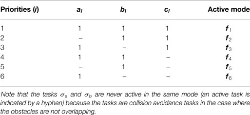
Table 6. Table illustrating the activation of mode in example 1.

The results of Example 1 are shown in Figure 5. The position task is fulfilled as predicted by the theory, i.e., the two waypoints are reached by the end effector. Figures 5A,B confirm this. In Figure 5B, it can be seen that the error between the actual and desired end position converges toward zero. Then, at around t = 12 s, the end effector is within the circle of acceptance of p_w1. Thus, the desired position switches to p_w2. The end effector immediately starts moving toward the new waypoint and converges to it at around t = 35 s. Furthermore, the end effector avoids the two obstacles by locking the distance to the obstacle center at the obstacle radius until the other active tasks drive the end effector away from the obstacle center on their own accord. This can be seen in Figure 5A, and it is also confirmed by Figure 5D: the set-based collision avoidance tasks never exceed the valid sets C_a and C_b, but freeze on the boundary of these sets.

FIGURE 5

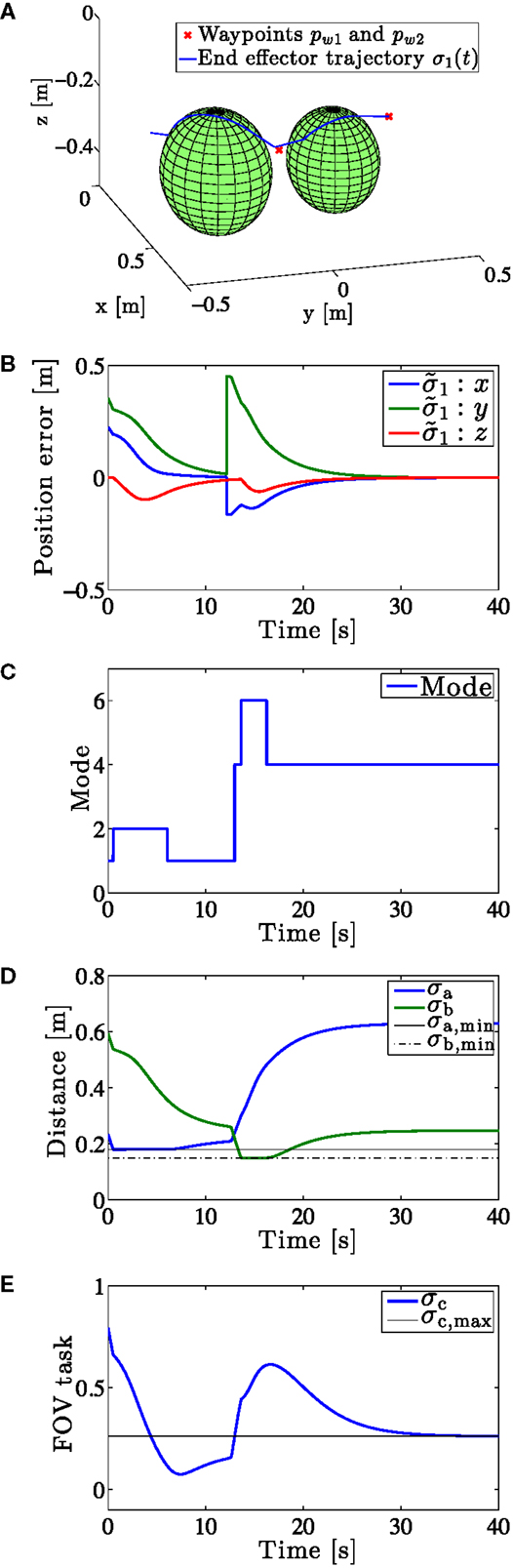
Figure 5. Logged data from Example 1. (A) End-effector trajectory. The two waypoints plotted in red. The figure shows that the end-effector moves around the obstacles to reach its desired position. (B) Position error ${\tilde{\mathrm{\sigma }}}_1$ in x, y, and z-direction. (C) Active mode over time. (D) End effector distance to the two obstacle centers. (E) Field of view task.

Figure 5C displays the active mode over time and confirms that mode changes coincide with set-based tasks either being activated (frozen on boundary/leaving valid set) or deactivated (unfrozen/approaching valid set). An increase in mode means that a new set-based task has been activated and vice versa.

Even though the initial condition of σ_c is outside C_c, the task is not active from t = 0 s because other, less restrictive modes, naturally bring the task closer to and eventually into C_c. However, at around t = 13 s, the system enters mode 4 and activates σ_c because mode 1–3 would all lead to σ_c leaving C_c. Due to the fact that σ_c is a low-priority set-based task, it still exceeds its maximum value in spite of the system activating the task, as predicted by the theory. However, by keeping the task active, eventually σ_c converges back to the boundary of C_c.

7.4. Example 2

In this example, the system has been given a time-varying trajectory for the end effector to track:

${\mathrm{\sigma }}_{1,\text{des}}\left(t\right)={\mathrm{\sigma }}_{\text{pos},\text{des}}\left(t\right)=\left[\begin{array}{c}\hfill 0.5{\sin }^2\left(0.1t\right)+0.2\hfill \\ \hfill 0.5\cos \left(0.1t\right)+0.25\sin \left(0.1t\right)\hfill \\ \hfill 0.5\sin \left(0.1t\right)\cos \left(0.1t\right)+0.1\hfill \end{array}\right]$ (127)

The task gain matrix has been chosen as

${\mathbf{\Lambda }}_{\text{pos}}=\text{diag}\left(\left[0.150.150.15\right]\right).$ (128)

In addition, the system is also given a valid workspace: a minimum and maximum value for the x, y and z position of the end effector. This is implemented as three set-based tasks that are equal to the first, second, and third element of σ _pos, respectively. These set-based tasks are all implemented as high-priority, as shown in the Table 7 below.

TABLE 7

Table 7. Implemented tasks in example 2 sorted by decreasing priority.

A system with 3 set-based tasks has 2³ = 8 modes to consider:

$\begin{array}{l}\hfill \text{Mode\hspace{0.17em}}1:{\dot{\mathit{\text{q}}}}_{\text{des}}={\mathit{\text{f}}}_1\triangleq {\mathit{\text{J}}}_1^{†}{\Lambda }_1{\tilde{\mathrm{\sigma }}}_1\end{array}$ (129)

$\begin{array}{l}\hfill \text{Mode\hspace{0.17em}}2:{\mathrm{\sigma }}_{\text{a}}\text{\hspace{0.17em}active},{\dot{\mathit{\text{q}}}}_{\text{des}}={\mathit{\text{f}}}_2\triangleq {\mathit{\text{N}}}_{\text{a}}{\mathit{\text{J}}}_1^{†}{\Lambda }_1{\tilde{\mathrm{\sigma }}}_1\end{array}$ (130)

$\begin{array}{l}\hfill \text{Mode\hspace{0.17em}}3:{\mathrm{\sigma }}_{\text{b}}\text{\hspace{0.17em}active},{\dot{\mathit{\text{q}}}}_{\text{des}}={\mathit{\text{f}}}_3\triangleq {\mathit{\text{N}}}_{\text{b}}{\mathit{\text{J}}}_1^{†}{\Lambda }_1{\tilde{\mathrm{\sigma }}}_1\end{array}$ (131)

$\begin{array}{l}\hfill \text{Mode\hspace{0.17em}}4:{\mathrm{\sigma }}_{\text{c}}\text{\hspace{0.17em}active},{\dot{\mathit{\text{q}}}}_{\text{des}}={\mathit{\text{f}}}_4\triangleq {\mathit{\text{N}}}_{\text{c}}{\mathit{\text{J}}}_1^{†}{\Lambda }_1{\tilde{\mathrm{\sigma }}}_1\end{array}$ (132)

$\begin{array}{l}\hfill \text{Mode\hspace{0.17em}}5:{\mathrm{\sigma }}_{\text{a}},{\mathrm{\sigma }}_{\text{b}}\text{\hspace{0.17em}active},{\dot{\mathit{\text{q}}}}_{\text{des}}={\mathit{\text{f}}}_5\triangleq {\mathit{\text{N}}}_{\text{ab}}^{\text{A}}{\mathit{\text{J}}}_1^{†}{\Lambda }_1{\tilde{\mathrm{\sigma }}}_1\end{array}$ (133)

$\begin{array}{l}\hfill \text{Mode\hspace{0.17em}}6:{\mathrm{\sigma }}_{\text{a}},{\mathrm{\sigma }}_{\text{c}}\text{\hspace{0.17em}active},{\dot{\mathit{\text{q}}}}_{\text{des}}={\mathit{\text{f}}}_6\triangleq {\mathit{\text{N}}}_{\text{ac}}^{\text{A}}{\mathit{\text{J}}}_1^{†}{\Lambda }_1{\tilde{\mathrm{\sigma }}}_1\end{array}$ (134)

$\begin{array}{l}\hfill \text{Mode\hspace{0.17em}}7:{\mathrm{\sigma }}_{\text{b}},{\mathrm{\sigma }}_{\text{c}}\text{\hspace{0.17em}active},{\dot{\mathit{\text{q}}}}_{\text{des}}={\mathit{\text{f}}}_7\triangleq {\mathit{\text{N}}}_{\text{bc}}^{\text{A}}{\mathit{\text{J}}}_1^{†}{\Lambda }_1{\tilde{\mathrm{\sigma }}}_1\end{array}$ (135)

$\begin{array}{l}\hfill \text{Mode\hspace{0.17em}}8:{\mathrm{\sigma }}_{\text{a}},{\mathrm{\sigma }}_{\text{b}},{\mathrm{\sigma }}_{\text{c}}\text{\hspace{0.17em}active},{\dot{\mathit{\text{q}}}}_{\text{des}}={\mathit{\text{f}}}_8\triangleq {\mathit{\text{N}}}_{\text{abc}}^{\text{A}}{\mathit{\text{J}}}_1^{†}{\Lambda }_1{\tilde{\mathrm{\sigma }}}_1\end{array}$ (136)

Denote the Boolean variables

$\begin{array}{ll}\hfill \begin{array}{rl}{\mathit{\varphi }}_i& \text{\hspace{0.17em}≜\hspace{0.17em}in\_T\_RC}\left({\mathit{\text{J}}}_{\mathit{\varphi }}{\mathit{\text{f}}}_i,{\mathrm{\sigma }}_{\mathit{\varphi }},{\mathrm{\sigma }}_{\mathit{\varphi },\text{min}},{\mathrm{\sigma }}_{\mathit{\varphi },\text{max}}\right)\\ & \text{for\hspace{0.17em}}i\in \left\{1,\dots ,8\right\}\text{\hspace{0.17em}and\hspace{0.17em}}\mathit{\varphi }\in \left\{\text{a},\dots ,\text{c}\right\}\end{array}& \end{array}$ (137)

The active mode is then chosen according to Table 8.

TABLE 8

Table 8. Table illustrating the activation of mode in example 2.

The results of Example 2 are shown in Figures 6 and 7. The system is unable to track the equality task perfectly, as the desired trajectory moves in and out of the allowed workspace (Figures 6A and 7). Mathematically, this is explained by the fact that the set-based tasks and the position equality task are not linearly independent (in fact, they are equal to each other). Thus, Assumption 1 is not fulfilled, and the equality task errors can no longer be guaranteed to converge to zero. However, as seen in Figure 6C, the end effector stays within the valid workspace at all times by freezing on the boundary when following the trajectory would bring it outside of the valid workspace. Figure 6B displays the active mode over time. Mode changes clearly correspond to set-based tasks being activated/deactivated on the border of their valid sets.

FIGURE 6

Figure 6. Logged data from example 2. (A) Desired and actual end trajectory plotted in red and blue, respectively. The allowed workspace is illustrated by the green box. Initial and end position marked by x and o, respectively. (B) Active mode over time. (C) Reference and actual end effector position in x, y, and z-direction with valid workspace limits.

FIGURE 7

Figure 7. Actual vs. desired end effector trajectory from example 1 plotted in the xy-, xz-, and yz-plane, respectively. A three-dimensional plot is given in Figure 6A.

Videos of the experimental results can be viewed online.¹

8. Conclusion

A general robotic system is controlled in joint space but has desired behavior (tasks) specified in task space. The singularity-robust multiple task-priority inverse kinematics framework has been developed as a way to generate a reference trajectory in joint space to fulfill several tasks in a prioritized order simultaneously. This framework has been developed for equality tasks, which are tasks that assign an exact desired value to the controlled variable (e.g., the end-effector configuration). However, for a general robotic system, several goals may be described as set-based tasks, i.e., tasks with a desired interval [area of satisfaction (Escande et al., 2014)]. Two classic, yet important examples are joint limits and obstacle avoidance. Additional examples are manipulability, dexterity, and field of view (for directional sensors, such as a camera mounted on the end effector).

This paper presents an extension to the singularity-robust multiple task-priority inverse kinematics framework that enables set-based tasks to be handled directly. The proposed method allows a general number of scalar set-based tasks to be handled with a given priority within a number of equality tasks. The main purpose of this method is to fulfill the system’s equality tasks while ensuring that the set-based tasks are always satisfied, i.e., contained in their valid set. A mathematical framework is presented and concluded with a stability analysis, in which it is proven that high-priority set-based tasks remain in their valid set at all times, whereas lower-priority set-based tasks cannot be guaranteed to be satisfied due to the influence of the higher-priority equality tasks. Furthermore, it is proven that the equality task errors converge asymptotically to zero given certain assumptions.

A practical implementation of the proposed algorithm is presented along with an analysis of the computational cost. Finally, experimental results are presented where two examples have been implemented on a UR5 manipulator. The experimental results confirm the theory and prove the validity of the proposed method for practical purposes.

Future work includes expanding the algorithm to achieve smooth transitions between switches while maintaining the strict priority of all tasks and still guaranteeing satisfaction of the high-priority set-based tasks.

Author Contributions

SM: writing the paper, developing the theory, and running experiments. GA: writing the paper, developing the theory, providing feedback to theoretical and experimental results, and feedback on written paper. ART: developing the theory and feedback on written paper. KYP: developing the theory, providing feedback to theoretical and experimental results, and feedback on written paper. JS: running experiments and feedback on written paper.

Conflict of Interest Statement

The authors declare that the research was conducted in the absence of any commercial or financial relationships that could be construed as a potential conflict of interest.

Funding

This work was supported by the Research Council of Norway through the Center of Excellence funding scheme, project number 223254, by the Italian Ministero dell’Istruzione, dell’Università e della Ricerca, PRIN 2010–2011 through the project MARIS (protocol 2010FBLHRJ) and by the European Community through the projects ARCAS (FP7-287617), EuRoC (FP7-608849), DexROV (H2020-635491), and AEROARMS (H2020-644271).

Footnote

1. ^https://www.dropbox.com/sh/x92agg4n7ly9hdc/AAC-xh8DyJM5X6jknJhyoJdca?dl=0

References

Antonelli, G. (2008). “Stability analysis for prioritized closed-loop inverse kinematic algorithms for redundant robotic systems,” in Proc. 2008 IEEE International Conference on Robotics and Automation (Pasadena, CA: IEEE), 1993–1998.

Google Scholar

Antonelli, G. (2009). Stability analysis for prioritized closed-loop inverse kinematic algorithms for redundant robotic systems. IEEE Trans. Robot. 25, 985–994. doi: 10.1109/TRO.2009.2017135

CrossRef Full Text | Google Scholar

Antonelli, G. (2014). Underwater Robots, 3rd Edn. Heidelberg: Springer Tracts in Advanced Robotics, Springer-Verlag.

Google Scholar

Antonelli, G., Arrichiello, F., and Chiaverini, S. (2008). The null-space-based behavioral control for autonomous robotic systems. J. Intell. Serv. Robot. 1, 27–39. doi:10.1007/s11370-007-0002-3

CrossRef Full Text | Google Scholar

Antonelli, G., Moe, S., and Pettersen, K. (2015). “Incorporating set-based control within the singularity-robust multiple task-priority inverse kinematics,” in Proc. 23th Mediterranean Conference on Control and Automation (Torremolinos: IEEE), 1132–1137.

Google Scholar

Azimian, H., Looi, T., and Drake, J. (2014). “Closed-loop inverse kinematics under inequality constraints: application to concentric-tube manipulators,” in Proc. 2014 IEEE/RSJ International Conference on Intelligent Robots and Systems (IROS 2014) (Chicago, IL: IEEE), 498–503.

Google Scholar

Baizid, K., Giglio, G., Pierri, F., Trujillo, M., Antonelli, G., Caccavale, F., et al. (2015). “Experiments on behavioral coordinated control of an unmanned aerial vehicle manipulator system,” in IEEE International Conference on Robotics and Automation (ICRA) (Seattle, WA: IEEE), 4680–4685.

Google Scholar

Buss, S. R. (2009). Introduction to Inverse Kinematics with Jacobian Transpose, Pseudoinverse and Damped Least Squares Methods. San Diego, CA: University of California. Available at: https://www.math.ucsd.edu/∼sbuss/ResearchWeb/ikmethods/iksurvey.pdf

Google Scholar

Chiaverini, S. (1997). Singularity-robust task-priority redundancy resolution for real-time kinematic control of robot manipulators. IEEE Trans. Robot. Autom. 13, 398–410. doi:10.1109/70.585902

CrossRef Full Text | Google Scholar

Chiaverini, S., Oriolo, G., and Walker, I. D. (2008). “Kinematically redundant manipulators,” in Springer Handbook of Robotics, eds B. Siciliano and O. Khatib (Heidelberg: Springer-Verlag), 245–268.

Google Scholar

de Lasa, M., Mordatch, I., and Hertzmann, A. (2010). Feature-based locomotion controllers. ACM Trans. Graph. 29, 131:1–131:10. doi:10.1145/1778765.1781157

CrossRef Full Text | Google Scholar

Escande, A., Mansard, N., and Wieber, P.-B. (2014). Hierarchical quadratic programming: fast online humanoid-robot motion generation. Int. J. Robot. Res. 33, 1006–1028. doi:10.1177/0278364914521306

CrossRef Full Text | Google Scholar

Faverjon, B., and Tournassoud, P. (1987). “A local based approach for path planning of manipulators with a high number of degrees of freedom,” in Proc. 1987 IEEE International Conference on Robotics and Automation (ICRA), Vol. 4 (Raleigh, NC: IEEE), 1152–1159.

Google Scholar

Goebel, R., Sanfelice, R., and Teel, A. (2012). Hybrid Dynamical Systems: Modeling, Stability, and Robustness. Princeton, NJ: Princeton University Press.

Google Scholar

Golub, G., and Van Loan, C. (1996). Matrix Computations, 3rd Edn. Baltimore, MD: The Johns Hopkins University Press.

Google Scholar

Ioannou, P., and Sun, J. (1996). Robust Adaptive Control. Upper River Saddle, NJ: Prentice Hall, Inc.

Google Scholar

Kanoun, O., Lamiraux, F., and Wieber, P. (2011). Kinematic control of redundant manipulators: generalizing the task-priority framework to inequality task. IEEE Trans. Robot. 27, 785–792. doi:10.1109/TRO.2011.2142450

CrossRef Full Text | Google Scholar

Khatib, O. (1986). Real-time obstacle avoidance for manipulators and mobile robots. Int. J. Robot. Res. 5, 90. doi:10.1177/027836498600500106

CrossRef Full Text | Google Scholar

Liégeois, A. (1977). Automatic supervisory control of the configuration and behavior of multibody mechanisms. IEEE Trans. Syst. Man Cybern. 7, 868–871. doi:10.1109/TSMC.1977.4309644

CrossRef Full Text | Google Scholar

Maciejewski, A., and Klein, C. (1985). Obstacle avoidance for kinematically redundant manipulators in dynamically varying environments. Int. J. Robot. Res. 4, 109–117. doi:10.1177/027836498500400308

CrossRef Full Text | Google Scholar

Mansard, N., and Chaumette, F. (2007). Task sequencing for high-level sensor- based control. IEEE Trans. Robot. Autom. 23, 60–72. doi:10.1109/TRO.2006.889487

CrossRef Full Text | Google Scholar

Mansard, N., Khatib, O., and Kheddar, A. (2009). A unified approach to integrate unilateral constraints in the stack of tasks. IEEE Trans. Robot. 25, 670–685. doi:10.1109/TRO.2009.2020345

CrossRef Full Text | Google Scholar

Moe, S., Antonelli, G., Pettersen, K. Y., and Schrimpf, J. (2015a). “Experimental results for set-based control within the singularity-robust multiple task-priority inverse kinematics framework,” in Proc. 2015 IEEE International Conference on Robotics and Biomimetics (ROBIO 2015) (Zhuhai).

Google Scholar

Moe, S., Teel, A., Antonelli, G., and Pettersen, K. (2015b). “Stability analysis for set-based control within the singularity-robust multiple task-priority inverse kinematics framework,” in Proc. 54th IEEE Conference on Decision and Control (Osaka).

Google Scholar

Nakamura, Y., Hanafusa, H., and Yoshikawa, T. (1987). Task-priority based redundancy control of robot manipulators. Int. J. Robot. Res. 6, 3–15. doi:10.1177/027836498700600103

CrossRef Full Text | Google Scholar

Siciliano, B. (1990). Kinematic control of redundant robot manipulators: a tutorial. J. Intell. Robot. Syst. 3, 201–212. doi:10.1007/BF00126069

CrossRef Full Text | Google Scholar

Siciliano, B., Sciavicco, L., Villani, L., and Oriolo, G. (2009). Robotics: Modelling, Planning and Control. Springer-Verlag.

Google Scholar

Siciliano, B., and Slotine, J.-J. (1991). “A general framework for managing multiple tasks in highly redundant robotic systems,” in Proc. 5th International Conference on Advanced Robotics (Pisa: IEEE), 1211–1216.

Google Scholar

Simetti, E., Casalino, G., Torelli, S., Sperindé, A., and Turetta, A. (2013). Floating underwater manipulation: developed control methodology and experimental validation within the TRIDENT project. J. Field Robot. 31, 364–385. doi:10.1002/rob.21497

CrossRef Full Text | Google Scholar

Spong, M., Hutchinson, S., and Vidyasagar, M. (2005). Robot Modeling and Control. Hoboken, NJ: Wiley.

Google Scholar

Whitney, D. (1969). Resolved motion rate control of manipulators and human prostheses. IEEE Trans. Man Mach. Syst. 10, 47–52. doi:10.1109/TMMS.1969.299896

CrossRef Full Text | Google Scholar

Wu, H., Tizzano, W., Andersen, T. T., Andersen, N. A., and Ravn, O. (2014). Hand-eye calibration and inverse kinematics of robot arm using neural network. Adv. Intell. Syst. Comput. 274, 581–591. doi:10.1007/978-3-319-05582-4_50

CrossRef Full Text | Google Scholar