Evaluating Morphological Computation in Muscle and DC-Motor Driven Models of Hopping Movements

1. Introduction

Morphological computation (MC), in the context of embodied (artificial) intelligence, refers to processes, which are conducted by the body (and environment) that otherwise would have to be performed by the brain (Pfeifer and Bongard, 2006). A nice example of MC is given by Wootton (1992) (see p. 188), who describes how “active muscular forces cannot entirely control the wing shape in flight. They can interact dynamically with the aerodynamic and inertial forces that the wings experience and with the wing’s own elasticity; the instantaneous results of these interactions are essentially determined by the architecture of the wing itself […]”

MC is relevant in the study of biological and robotic systems. To illustrate the utility of MC in robotics, we will first briefly discuss the Passive Dynamic Walker (McGeer, 1990), which is a purely mechanical system. The proportions of the legs and the weight distribution are similar to those of human legs. The Passive Dynamic Walker shows that walking can result from the interaction of the system’s physical properties and its environment (in this case a slope of 3°). No actuation is required for the walking behavior. Transferred to robotics, this means that systems with high morphological computation only need to generate motor commands when they are needed. Not only does such a control increase the durability of the systems (because the wear-out of the actuators is decreased), it also means that robots with high MC will have a reduced energy demand for their actuation (e.g., Niiyama et al. (2012) and Renjewski et al. (2015)). By outsourcing computation to the embodiment, the controller complexity, and hence, the computational cost can be reduced, which again contributes to the overall reduction of the energy consumption. For contemporary mobile robots, the energy supply still is one of the biggest unsolved problems, as mobile robots can either operate only for a short period of time or have to carry heavy batteries (Baughman, 2005). To summarize, increasing MC for a robotic system potentially decreases the overall energy demand, the controller complexity, and finally also the wear-out of the system.

This said, one should not mistake MC to be synonymous for energy efficiency. One example in which MC does not relate to energy efficiency is human running, in particular, running in an outdoor environment, such as a downhill off-road path. The runner is not able to detect every change of slope or see every stone, tree branch, etc., on the ground. This means that most irregularities are sensed at the moment when the foot touches the ground (Müller et al., 2015). However, an immediate reaction in the sense of neural change in muscle activity is not possible, as the communication pathway from the feet to the spinal cord and back is simply too long (~0.02 s). Running on an irregular ground is only possible because of the physical properties of the muscle-tendon system. Not only do they have a shock-absorbing function, within certain limits, irregularities of the ground can be accounted for without any explicit control (Brown et al., 1995; Proctor and Holmes, 2010; Müller et al., 2015). In this case, MC does not contribute to the energy efficiency (running is not energy efficient), but it is required to enable the behavior. We believe that maximizing MC covers more than just energy efficiency (fast adaptivity in uncertain environments is one example), but that this is an immediate benefit in the field of robotics.

For biological systems, energy efficiency and adaptivity are important and evolutionary advantages. A strong indication for the importance of energy efficiency is given by the fact that the human brain accounts for only 2% of the body mass but is responsible for 20% of the entire energy consumption (Clark and Sokoloff, 1999). The energy consumption is also remarkably constant (Sokoloff et al., 1955). Under the assumption that the acquisition of energy was not a trivial task throughout most of the evolution of humans, on can safely conclude that as much computation as possible has been outsourced to the embodiment. When hunting prey or escaping from a predator, adaptivity to irregularities in the environment through morphological properties is a clear evolutionary advantage. Therefore, MC may be a driving force in evolution.

In biological systems, movements are typically generated by muscles. Several simulation studies have shown that the muscles’ typical non-linear contraction dynamics can be exploited in movement generation with very simple control strategies (Schmitt and Haeufle, 2015). Muscles improve movement stability in comparison to torque driven models (van Soest and Bobbert, 1993) or simplified linearized muscle models [for an overview see (Haeufle et al., 2012)]. Muscles also reduce the influence of the controller on the actual kinematics (they can act as a low-pass filter). This means that the hopping kinematics of the system is more predetermined with non-linear muscle characteristics than with simplified linear muscle characteristics (Haeufle et al., 2012). And finally, in hopping movements, muscles reduce the control effort (amount of information required to control the movement) by a factor of approximately 20 in comparison to a DC-motor driven movement (Haeufle et al., 2014).

In view of these results, we expect that MC plays an important role in the control of muscle driven movement. To study this quantitatively, a suitable measure for MC is required. There are several approaches to formalize MC. Hauser et al. (2011) proposes a dynamical systems approach in which the effect of the morphology on the attractor landscape of the systems is taken into account. Polani (2011) minimizes the controller complexity in a reinforcement learning setting. This is very close to our second quantification MC_MI (see Section 3.2). The difference is that we take the behavior complexity instead of a reward signal into account. Rückert and Neumann (2013) measure morphological computation indirectly by measuring how changes of the morphology reduce or increase the required controller complexity in the context of stochastic optimal control.

In our previous work, we have focused on a direct quantification of the embodiment, whereas most other approaches quantify MC indirectly through the controller complexity. In particular, in our first publication (Zahedi and Ay, 2013), we focused on an agent-centric perspective of measuring MC. We had proposed two different, complementary concepts of measuring morphological computation (which are discussed below). From those concepts, which rely on information that is only partially available to the agent, we derived quantifications that only rely on the agents sensors and actuators. In this publication, we evaluate MC on simulated muscles models, which means that we have access to the full system’s state. Hence, in this publication, we concentrate on measures, which operate on the full system’s state. This allows us to investigate how the concepts operate on realistic muscle models without taking approximation errors into account that occur from limited sensor information. In a different publication (Ghazi-Zahedi and Rauh, 2015), we applied an information decomposition (Bertschinger et al., 2014) to the sensorimotor loop and developed a refined understand the two concepts that we have proposed in Zahedi and Ay (2013). Both publications used a binary toy world model to evaluate the measures. With this toy model, it was possible to show that these measures capture the conceptual idea of MC and, in consequence, that they are candidates to measure MC in more complex and more realistic systems.

The main contribution of this publication is to evaluate two measures of MC on biologically realistic hopping models. With this, we want to demonstrate their applicability in non-trivial, realistic scenarios. Based on our previous findings (see above), we hypothesize that MC is higher in hopping movements driven by a non-linear muscle compared to those driven by a simplified linear muscle or a DC-motor. Furthermore, our experiments show that a state-dependent analysis of MC for the different models leads to insights, which cannot be gained from the averaged measures alone. Finally, we provide detailed instructions on how to apply these measures to robotic systems and to computer simulations, including MATLAB^®, C++ code, and the data used in this publication (Ghazi-Zahedi, 2016). With this, we hope to provide a tool for the evaluation of MC in a large variety of applications.

The quantifications of MC require a formal representation of the sensorimotor loop (see Figure 1), which is introduced in the next section as far as it is required to understand the remainder of this work. For further information, the reader is referred to Klyubin et al. (2004), Zahedi et al. (2010), Ay and Zahedi (2013), and Zahedi and Ay (2013).

FIGURE 1

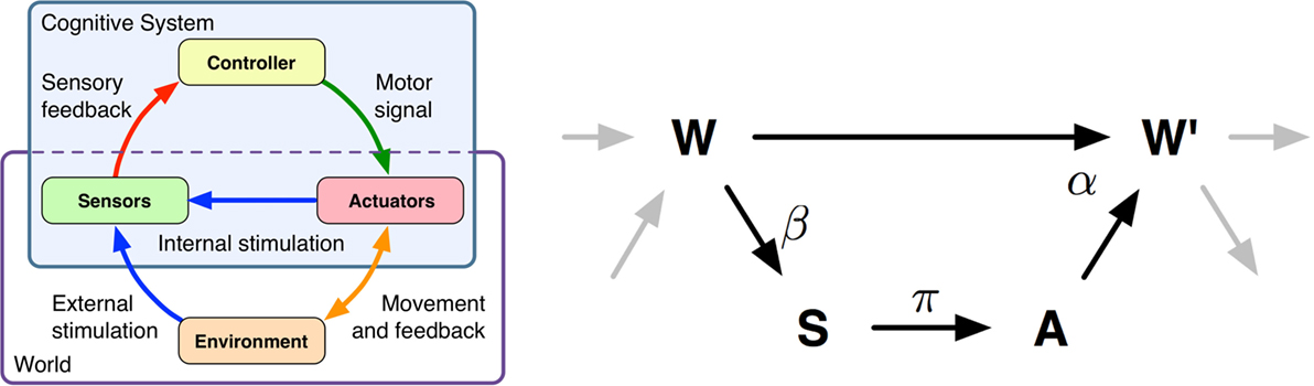
Figure 1. Left-hand side: Schematics of a cognitive system and the interactions of sensors, brain, actuators, and environment. Right-hand side: Causal model of the sensorimotor loop for a reactive system (no internal state). This figure depicts a single step of an embodied, reactive system’s sensorimotor loop. The state of the world, sensors, and actuators are modeled by the random variables W, S, and A. The arrows between the variables depict the causal relations. The Greek letters denote the corresponding kernels. The sensor kernel β(s|w) determines how the agent senses the world. The policy is given by π(a|s), and finally the world dynamics kernel α(w′|w, a) determines how the next world state W′ depends on the previous world state W and action A. A detailed explanation is given in Section 2.

2. The Sensorimotor Loop

The conceptual idea of the sensorimotor loop is similar to the basic control loop systematics, which is the basis of robotics and also of computer simulations of human movement. In our understanding, a cognitive system consists of a brain or controller, which sends signals to the system’s actuators, thereby affecting the system’s environment. We prefer to capture the body and environment in a single random variable named world. This is consistent with other concepts of agent-environment distinctions. An example for such a distinction can be found in the context of reinforcement learning, where the environment (world) is everything that cannot be changed arbitrarily by the agent (Sutton and Barto, 1998). A more thorough discussion of the brain-body-environment distinction can be found in (von Uexkuell, 1934; Clark, 1996) and more recently by Ay and Löhr (2015). A brief example of a world, based on a robot simulation, is given below. The loop is closed as the system acquires information about its internal state (e.g., current pose) and its world through its sensors.

For simplicity, we only discuss the sensorimotor loop for reactive systems in this work (for a detailed discussion, please see Ay and Zahedi (2014)). This is plausible, because behaviors which exploit the embodiment (e.g., walking, swimming, flying) are typically reactive. A measure that takes the controller state into account is discussed in Zahedi and Ay (2013). Restricting ourselves to reactive systems results in three (stochastic) processes S(t), A(t), and W (t), $t\mathrm{\in }\mathbb{N}$ that constitute the sensorimotor loop (see Figure 1), which take values s, a, and w, in the sensor, actuator, and world state spaces (their respective domains will be clear from the context). The directed edges (see Figure 1) reflect causal dependencies between these random variables. We consider time to be discrete, i.e., $t\mathrm{\in }\mathbb{N}$ and are interested in what happens in a single time step. Therefore, we use the following notation. Random variables without any time index refer to some fixed time t and primed variables to time t + 1, i.e., the two variables S, S′ refer to S(t) and S(t + 1).

Starting with the initial distribution over world states, denoted by p(w), the sensorimotor loop for reactive systems is given by three conditional probability distributions, β, α, π, also referred to as kernels. The sensor kernel, which determines how the agent perceives the world, is denoted by β(s|w), the agent’s controller or policy is denoted by π(a|s), and finally, the world dynamics kernel is denoted by α(w′|w,a).

To understand the function of the world dynamics kernel α(w′|w,a), it is useful to think of a robotic simulation. In this scenario, the world state W is the state of the simulator at a given time step, which includes the pose of all objects, their velocities, applied forces, etc. The actuator state A is the value that the controller passes on to the physics engine prior to the next physics update. Hence, the world dynamics kernel α(w′|w,a) is closely related to the forward model that is known in the context of robotics and biomechanics.

Based on this notation, we can now formulate quantifications of MC in the next section.

3. Quantifying Morphological Computation

In the introduction, we stated that MC relates to the computation that the body (and environment) performs that otherwise would have to be conducted by the controller (or brain). This means that we want to measure the extent to which the system’s behavior is the result of the world dynamics (i.e., the body’s internal dynamics and it’s interaction with its world) and how much of the behavior is determined by the policy π (see Figure 1). In our previous publication (Zahedi and Ay, 2013), we have derived two complementary concepts to quantify MC (see Section 1 for a discussion). The two measures discussed below were chosen for presentation in this work, because they represent the two concepts.

3.1. Morphological Computation as Conditional Mutual Information (MC_W)

The first quantification, which is used in this work, was introduced in Zahedi and Ay (2013). The idea behind it can be summarized in the following way. The world dynamics kernel α(w′|w,a) captures the influence of the actuator signal A and the previous world state W on the next world state W′. A complete lack of MC would mean that the behavior of the system is entirely determined by the system’s controller, and hence, by the actuator state A. In this case, the world dynamics kernel reduces to p(w′|a). Every difference from this assumption means that the previous world state W had an influence, and hence, information about W changes the distribution over the next world states W′. The discrepancy of these two distributions can be measured with the average of the Kullback-Leibler divergence D_KL(α(w′|w,a) || p(w′|a)), which is also known as the conditional mutual information I(W′;W|A). This distance is formally given by (see also Algorithm 2)

${\text{MC}}_{\text{W}}:={\displaystyle \sum _{w\prime ,w,a}}p\left(w\prime ,w,a\right){\log }_2\frac{\mathrm{\alpha }\left(w\prime |w,a\right)}{p\left(w\prime |a\right)}.$ (1)

3.2. Morphological Computation as Comparison of Behavior and Controller Complexity (MC_MI)

The second quantification follows concept one of Zahedi and Ay (2013). The assumption that underlies this concept is that, for a given behavior, MC decreases with an increasing effect of the action A on the next world state W′. The corresponding measure MC_A ∝–$I\left(W\prime ;W|A\right)$ cannot be used in systems with deterministic policy, because for these systems $I\left(W\prime ;W|A\right)$ = 0 (see Appendix A). Therefore, for this publication, we require an adaptation that operates on world states and is applicable to deterministic systems.

The new measure compares the complexity of the behavior with the complexity of the controller. The complexity of the behavior can be measured by the mutual information of consecutive world states, I(W′;W), and the complexity of the controller can be measured by the mutual information of sensor and actuator states, $I\left(A;S\right)$, for the following reason. The mutual information of two random variables can also be written as difference of entropies: $I\left(X;Y\right)$ = H(X) − H(X|Y), H(X) = −∑_xp(x)log₂ p(x), H(X|Y) = −∑_x,y p(x, y) log₂ p(x|y), which, applied to our setting, means that the mutual information I(W′;W) is high, if we have a high entropy over world states W′ (first term) that are highly predicable (second term). Summarized, this means that the mutual information I(W′;W) is high if the system shows a diverse but non-random behavior. Obviously, this is what we would like to see in an embodied system. On the other hand, a system with high MC should produce a complex behavior based on a controller with low complexity. Hence, we want to reduce the mutual information $I\left(A;S\right)$, because this either means that the policy has a low diversity in its output (low entropy over actuator states H(A)) or that there is only a very low correlation between sensor states S and actuator states A (high conditional entropy H(A|S)). Therefore, we define the second measure as the difference of these two terms, which is (see also Algorithm 4).

${\text{MC}}_{\text{MI}}=I\left(W\prime ;W\right)-I\left(A;S\right).$ (2)

Equation 2 reveals that this measure is closely related to the work by Polani (2011), and in particular his work on relevant information (Polani et al., 2006), which minimizes the controller complexity while maximizing a reward function, i.e., min $\left(I\right(S;A)-\mathrm{\beta }\mathbb{E}\mathrm{\{}Q\mathrm{(}s,a\mathrm{)\})}$.

For deterministic systems, as those studied in this work, the two proposed measures, MC_W and MC_MI [see equations (1) and (2)], are closely related. In particular, it holds that MC_W − MC_MI = H(A|W′) (see Appendix B). The inequality MC_W ≥ MC_MI may not be satisfied always, because discretization can introduce stochasticity.

Note that in the case of a passive observer, i.e., a system that observes the world but in which there is no causal dependency between the action and the next world state (i.e., missing connection between A and W′ in Figure 1), the controller complexity $I\left(A;S\right)$ in equation (2) will reduce the amount of MC measured by MC_MI, although the actuator state does not influence the world dynamics. This might be perceived as a potential shortcoming. In the context discussed in this paper, e.g., data recorded from biological or robotic systems, we think that this will not be an issue.

The next section introduces the hopping models on which the two measures are evaluated.

3.3. Algorithms

This section presents the algorithms to calculate both measures in pseudo-code. Implementations of the algorithms in MATLAB^® and C++ are available at Ghazi-Zahedi (2016). The repository also contains the data sets used in this publication.

Note that we use a compressed notion in Algorithms 2–5, in which x′ = x(t + 1) and x = x(t).

The first algorithm (see Algorithm 1) is required to pre-process the data. Currently, our measure only work on discretized data. This means that we need to bin the system’s variables (position, velocity, etc.), and furthermore, combine to a uni-variate random variable W. The same procedure must also be followed for the action state variable A and sensor state variable S.

ALGORITHM 1

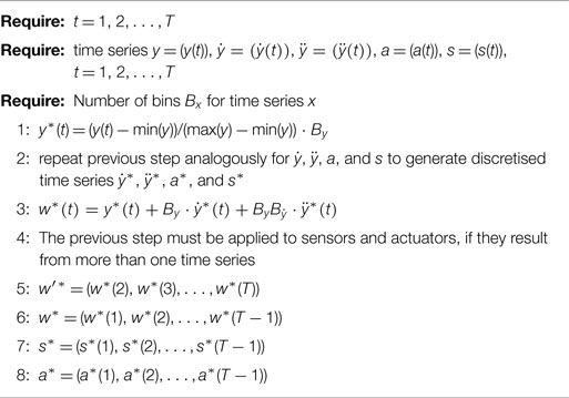
Algorithm 1. Discretisation of the data. This part is the same for all measures, depending on which time series are required. The minimum and maximum were determined of the data of all hopping models.

Once the discretised uni-variate random variables W, A, S, W′ are available, we can now calculate the two measures MC_W (see Algorithm 2) and MC_MI (see Algorithm 4).

ALGORITHM 2

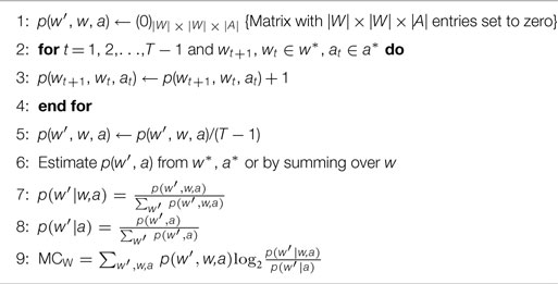
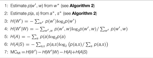
Algorithm 2. Algorithm for MC_W.

The state-dependent calculations of the two measures on require minimal changes to the original algorithms. Instead of averaging over all states, which leads to a single number as a result, the measures are evaluated n-tupel in the data set. This means that for MC_W, the logarithm is evaluated for every triple w_t+1, w_t, a_t (see Algorithm 3). Consequently, the logarithms that are used in the measure MC_MI are evaluated for every 4-tupel w_t+1, w_t, a_t, s_t in the data set. The arithmetic mean ($\frac{1}{n}\sum x_t$, where x_t is either MC_W(t) or MC_MI(t), see Algorithms 3 and 5) of the state-dependent MC values leads to same values that result from the original algorithms.

ALGORITHM 3

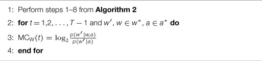
Algorithm 3. Algorithm for state-dependent MC_W(t).

ALGORITHM 4

Algorithm 4. Algorithm for MC_MI.

ALGORITHM 5

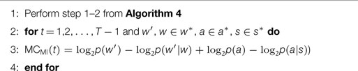
Algorithm 5. Algorithm for state-dependent MC_MI(t).

This concludes the discussion of the measures and their implementation. The next section presents the muscle and DC-motor model against which these measure were evaluated.

4. Hopping Models

In a reduced model, hopping motions can be described by a one-dimensional differential equation (Haeufle et al., 2010):

$m\ddot{y}=-\mathit{mg}+\left\{\begin{array}{cc}0\hfill & y>l_0\text{flight phase}\hfill \\ F_{\text{L}}\hfill & y\le l_0\text{ground contact}\hfill \end{array}\right.,$ (3)

where the point mass m = 80 kg represents the total mass of the hopper, which is accelerated by the gravitational force (g = –9.81 m/s²) in negative y-direction. An opposing leg force F_L in positive y-direction can act only during ground contact (y ≤ l₀ = 1 m). Hopping motions are then characterized by alternating flight and stance phases. For this manuscript, we investigated three different models for the leg force (Figure 2). All models have in common, that the leg force depends on a control signal u(t) and the system state y(t), $\dot{y}\left(t\right)$: $F_{\text{L}}=F_{\text{L}}\left(u\left(t\right),y\left(t\right),\dot{y}\left(t\right)\right)$, meaning, that the force modulation partially depends on the controller output u(t) and partially on the dynamic characteristics, or material properties of the actuator. The control parameters of all three models were adjusted to generate the same periodic hopping height of max (y(t)) = 1.070 m. All models were implemented in MATLAB^® Simulink™ (Ver2014b) and solved with ode45 Dormand-Prince variable time step solver with absolute and relative tolerances of 10⁻¹². To evaluate and compare the results of the models, a time-discrete output with constant sampling frequency is required (see Section 3.3). Therefore, the quasi-continuous variable time step signals generated by the ode45 solver are not adequate. To generate the desired output at 1 kHz sampling frequency, we used the Simulink built-in feature to generate desired output only. This way, the solver decreased step-size below 1 ms if required for precision, however, Simulink would only output the data for 1 kHz sampling frequency. This is similar to measuring a continuous physical system with a discrete time sensor. The models were solved for T = 8 s.

FIGURE 2

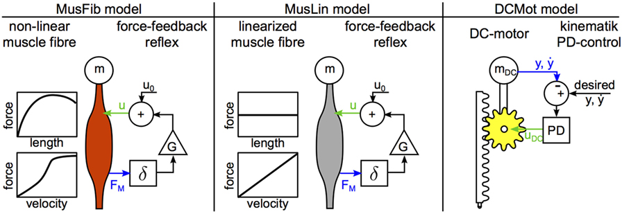
Figure 2. Hopping models. The MusFib model considers the non-linear contraction dynamics of active muscle fibers and is driven by a mono-synaptic force-feedback reflex. The MusLin model only differs in the contraction dynamics, where the force-length relation is neglected and the force-velocity relation is approximated linearly. The DCMot model generates the leg force with a DC motor. It is controlled by a proportional-differential controller (PD), enforcing the desired trajectory. The desired trajectory is the recorded trajectory from the MusFib Model. The sensor signals are shown as blue arrows, and the actuator control signals are shown as green arrows. In case of the muscle models, the sensor signal is the muscle force F_M, and the actuator control signal is the neural muscle stimulation u. In case of the DC-motor model, the sensor signals are the position and velocity of the mass, and the actuator control signal is the motor armature voltage u_DC.

4.1. Muscle-Fiber Model (MusFib)

A biological muscle generates its active force in muscle fibers whose contraction dynamics are well studied. It was found that the contraction dynamics are qualitatively and quantitatively (with some normalizations) very similar across muscles of all sizes and across many species. In the MusFib model, the leg force is modeled to incorporate the active muscle fibers’ contraction dynamics. The model has been motivated and described in detail elsewhere (Haeufle et al., 2010, 2012, 2014). In a nutshell, the material properties of the muscle fibers are characterized by two terms modulating the leg force

$F_{L,\text{MusFib}}=q\left(t\right)F_{\text{fib}}\left(l_M,{\dot{l}}_M\right).$ (4)

The first term q(t) represents the muscle activity. The activity depends on the neural stimulation u(t) of the muscle 0.001 ≤ u(t) ≤ 1 and is governed by biochemical processes modeled as a first-order ODE called activation dynamics

$\dot{q\left(t\right)}=\frac{1}{\mathrm{\tau }}\left(u\left(t\right)-q\left(t\right)\right),$ (5)

with the time constant τ = 10 ms. The second term in equation (5) F_fib considers the force-length and force-velocity relation of biological muscle fibers. It is a function of the system state, i.e., the muscle length l_M = y and muscle contraction velocity ${\dot{l}}_M=\dot{y}$ during ground contact y ≤ l₀ and constant l_M = l₀ ${\dot{l}}_M=0$ during flight y > l₀:

$F_{\text{fib}}=F_{\max }\cdot \exp \left(-c{\left|\frac{l_M-l_{\text{opt}}}{l_{\text{opt}}w}\right|}^3\right)\times \left\{\begin{array}{cc}\frac{{\dot{l}}_{M,\text{max}}+{\dot{l}}_M}{{\dot{l}}_{M,\text{max}}-K{\dot{l}}_M}\hfill & {\dot{l}}_M>0\hfill \\ N+\left(N-1\right)\frac{{\dot{l}}_{M,\text{max}}-{\dot{l}}_M}{-7.56K{\dot{l}}_M-{\dot{l}}_{M,\text{max}}}\hfill & {\dot{l}}_M\le 0\hfill \end{array}\right..$ (6)

Here, we use a maximum isometric muscle force F_max = 2.5 kN, an optimal muscle length l_opt = 0.9 m, force-length parameters w = 0.45 m and c = 30, and force-velocity parameters ${\dot{l}}_{\mathit{max}}=-3.5m{s}^{-1}$, K = 1.5, and N = 1.5 (Haeufle et al., 2010).

In this model, periodic hopping is generated with a controller representing a mono-synaptic force-feedback. The neural muscle stimulation

$u\left(t\right)=G\cdot F_{L,\text{MusFib}}\left(t-\mathrm{\delta }\right)+u_0$ (7)

is based on the time delayed (δ = 15 ms) muscle fiber force F_L,MusFib. Please note that this delay corresponds to the biophysical time delay due to the signal propagation velocity of neurons. The feedback gain is G = 2.4/F_max, and the stimulation at touch down u₀ = 0.027.

This model neither considers leg geometry nor tendon elasticity and is therefore the simplest hopping model with muscle-fiber-like contraction dynamics. The model output was the world state $w\left(t\right)=\left(y\left(t\right),\dot{y}\left(t\right),\ddot{y}\left(t\right)\right)$, the sensor state s(t) = F_L,MusFib(t), and the neural control command a(t) = u(t). For this model, these are the values that the random variables W, S, and A take at each time step.

4.2. Linearized Muscle-Fiber Model (MusLin)

This model differs from the model MusFib only in the representation of the force–length–velocity relation, i.e., $F_{L,\text{MusLin}}=q\left(t\right)F_{\text{lin}}\left({\dot{l}}_M\right)$ [see equation (6)]. More precisely, the force–length relation is neglected and the force–velocity relation is approximated linearly

$F_{\text{lin}}=1\cdot \left(1-\mathrm{\mu }{\dot{l}}_M\right),$ (8)

with μ = 0.25 m/s. Feedback gain G = 0.8/F_max and stimulation at touch down u₀ = 0.19 were chosen to achieve the same hopping height as the MusFib model.

4.3. DC-Motor Model (DCMot)

An approach to mimic biological movement in a technical system (robot) is to track recorded kinematic trajectories with electric motors and a PD-control approach. The DCMot model implements this approach [slightly modified from Haeufle et al. (2014)]. The leg force generated by the DC-motor was modeled as

$F_{L,\text{DCMot}}=\mathrm{\gamma }{T}_{\mathit{DC}}=\mathrm{\gamma }{k}_T{I}_{\mathit{DC}},$ (9)

where k_T = 0.126 Nm/A is the motor constant, I_DC the current through the motor windings, γ = 100:1 the ratio of an ideal gear translating the rotational torque T_DC and movement $\dot{\mathrm{\phi }}\left(t\right)=\mathrm{\gamma }\dot{y}\left(t\right)$ of the motor to the translational leg force and movement required for hopping. The electrical characteristics of the motor can be modeled as

${\dot{I}}_{\mathit{DC}}=\frac{1}{L}\left(u_{\mathit{DC}}-k_T\mathrm{\gamma }\dot{y}\left(t\right)-R{I}_{\mathit{DC}}\right),$ (10)

where –48 V ≤ u_DC ≤ 48 V is the armature voltage (control signal), R = 7.19Ω the resistance, and L = 1.6 mH the inductance of the motor windings. The motor parameters were taken from a commercially available DC-motor commonly used in robotics applications (Maxon EC-max 40, nominal Torque T_nominal = 0.212 Nm). As this relatively small motor would not be able to lift the same mass, the body mass was adapted to guarantee comparable accelerations

$m_{\mathit{DC}}=\frac{\mathrm{\gamma }{T}_{\text{nominal}}}{F_{\max }}m=0.68\mathit{kg}.$ (11)

The controller implemented in this technical model is a standard PD-controller. The controller tries to minimize the error between a desired kinematic trajectory (y_des(t) and ${\dot{y}}_{\text{des}}\left(t\right)$) and the actual position and velocity (y(t) and $\dot{y}\left(t\right)$) by adapting the motor voltage:

$u_{\mathit{DC}}\left(t\right)=K_P\left(y_{\text{des}}\left(t\right)-y\left(t\right)\right)+K_D\left({\dot{y}}_{\text{des}}\left(t\right)-\dot{y}\left(t\right)\right).$ (12)

Here, the feedback gains are K_P = 5000 V/m and K_D = 500 Vs/m. The desired trajectory during ground contact was taken from the periodic hopping trajectory of the MusFib model (y_des(t) = y_MusFib(t) and ${\dot{y}}_{\text{des}}\left(t\right)={\dot{y}}_{\text{MusFib}}\left(t\right)$).

This model is the simplest implementation of negative feedback control that allows to enforce a desired hopping trajectory on a technical system. The model output was the world state $w\left(t\right)=\left(y\left(t\right),\dot{y}\left(t\right),\ddot{y}\left(t\right)\right)$, the sensor state $s\left(t\right)=\left(y\left(t\right),\dot{y}\left(t\right)\right)$, and the actuator control command a(t) = u_DC(t).

5. Experiments

This section discusses the experiments that were conducted with the hopping models and the preprocessing of the data. Algorithms for the calculations are provided in the previous section (Section 3). At this stage, the measures operate on discrete state spaces [see equations (1)–(4) and Algorithms 2–4]. Hence, the data was discretized in the following way. To ensure the comparability of the results, the domain (range of values) for each variable (e.g., the position y) was calculated over all hopping models. Then, the data of each variable was discretized into 300 values (bins). The algorithm for the discretization is described in Algorithm 1. Different binning resolutions were evaluated, and the most stable results were found for more than 100 bins. Finding the optimal binning resolution is a problem of itself and beyond the scope of this work. In practice, however, a reasonable binning can be found by increasing the binning until further increase has little influence on the outcome of the measures.

The possible range of actuator values is different for the motor and muscle models. For the muscle models, the values are in the unit interval, i.e., a(t) ∈ [0,1], whereas the values for the motor can have higher values (see above). Hence, to ensure comparability, we normalized the actions of the motor to the unit interval before they were discretized.

The hopping models are deterministic, which means that only a few hopping cycles are necessary to estimate the required probability distributions. To ensure comparability of the results, we parameterized the hopping models to achieve the same hopping height.

6. Results

The following paragraphs discuss the findings based on the averaged results presented in Table 1 first and then follow with a discussion of the state-dependent results presented in Figure 3.

TABLE 1

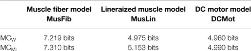
Table 1. Numerical results on the hopping models for MC_W [Morphological Computation as Conditional Mutual Information, see equation (14)] and MC_MI [Morphological Computation as the comparison between behavior and controller complexity, see equation (2)].

FIGURE 3

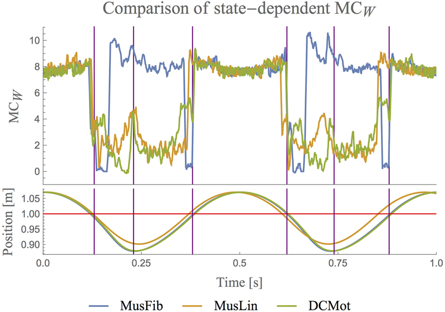
Figure 3. Comparison of state-dependent MC_W on the three hopping models (upper plot). The lower plot visualizes the hopping position. The red line separates stance and flight phases. The plots only show a small fraction of the recorded data. The full data is shown in Figure 4. For better readability, all the plots for MC are smoothened with a moving average of block size 5. The plots show that MC is high during the flight phase for all systems, i.e., whenever the behavior of the system is only governed by gravity. Only for the MusFib, MC is highest when the muscle is contracting. The other two models show low MC when the muscle is contracting and in general when the hopper touches the ground.

All three models generated a similar movement, i.e., periodic hopping with a hopping height of 1.07 m. However, the control signals and the trajectories of the center of mass vary between models (Figure 4). Therefore, the computed values for the morphological computation (MC) vary between the models for both quantification methods (Table 1). Compared to the complex muscle fiber model (MusFib), the linearized muscle model (MusLin) and the technical DC-motor model (DCMot) result in significantly lower values of MC (≈30% less, see Table 1).

FIGURE 4

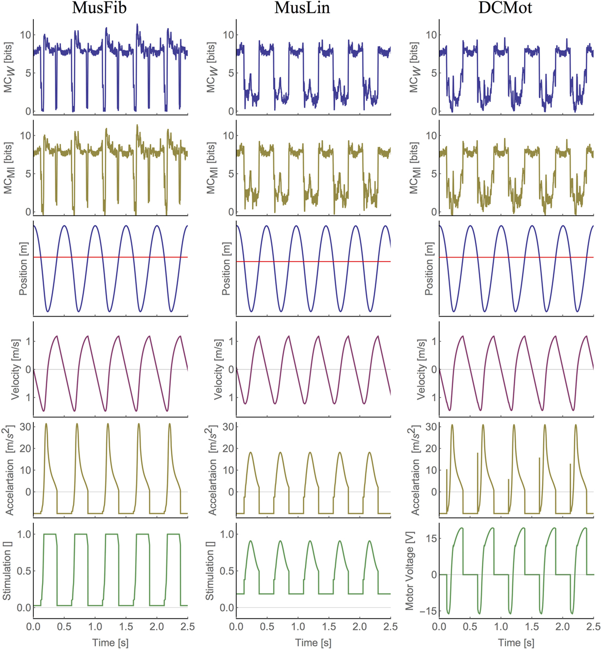
Figure 4. Plots of state-dependent MC (first two rows) and the world state (following four rows) for all muscle models. The red line in the position plot indicates the time steps at which the hopper touches ground (position is below the red line). Note that the stimulation is dimensionless.

To analyze the differences between the models in more detail, we plotted the state-dependent MC (see Algorithm 3). Figure 3 shows the values of MC_W for each state of the models during two hopping cycles. We chose to discuss MC_W only, because the corresponding values of MC_MI are very similar to those of MC_W, and hence, a discussion of the state-dependent MC_MI will not provide any additional insights. The plots for all models and the entire data are shown in Figure 4.

The orange line shows the state-dependent MC for the linear muscle model (MusLin) and the blue line for the non-linear muscle model (MusFib). The green line shows the state-dependent MC for the motor model (DCMot). In the figure, the lower lines show the position y of the center of mass over time. The PD-controller of the DCMot model is parameterized to follow the trajectory of the MusFib model, which is why the blue and green position plots coincide. The original data is shown in Figure 4. There are basically three phases, which need to be distinguished (indicated by the vertical lines). First, the flight phase, during which the hopper does not touch the ground (position plots are above the red line), second, the deceleration phase, which occurs after landing (position is below the red line but still declining), and finally, the acceleration phase, in which the position is below the red line but increasing.

The first observation is that MC is very similar for all models during most of the flight phase (position above the red line) and that it is proportional to the velocity of the systems. By that we mean that MC decreases when the velocity during flight decreases and increases when the system’s speed (toward the ground) increases. During flight, the behavior of the system is governed only by the interaction of the body (mass, velocity) and the environment (gravity) and not by the actuator models. Also, all actuator control signals are constant during flight. This explains why the values coincide for the three models.

For all models, MC drops as soon as the systems touch the ground. DCMot and MusLin reach their highest values only during the flight phase, which can be expected at least from a motor model that is not designed to exploit MC. The graphs also reveal that the MusLin model shows slightly higher MC around mid-stance phase, compared to the DCMot model. For the non-linear muscle model, the behavior is different. Shortly after touching the ground, the system shows a strong decline of MC, which is followed by a strong incline during the deceleration with the muscle. Contrary to the other two models, the non-linear muscle model MusFib shows the highest values when the muscle is contracted the most (until mid-stance). This is an interesting result, as it shows that the non-linear muscle is capable of showing more MC while the muscle is operating, compared to the flight phase, in which the behavior is only determined by the interaction of the body and environment.

7. Discussion

This work presented two different quantifications of morphological computation including algorithms, MATLAB^®, and C++ code to use them (Ghazi-Zahedi, 2016). We demonstrated their applicability in experiments with non-trivial, biologically realistic hopping models and discussed the importance of a state-based analysis of morphological computation. The first quantification, MC_W, measures MC as the conditional mutual information of the world and actuator states. Morphological computation is the additional information that the previous world state W provides about the next world state W′, given that the current actuator state A is known. The second quantification, MC_MI, compares the behavior and controller complexity to determine the amount of MC.

The numerical results of the two quantifications MC_W and MC_MI confirm our hypothesis that the MusFib model should show significantly higher MC, compared to the two other models (MusLin, DCMot). These results complement previous findings showing that the minimum information required to generate hopping is reduced by the material properties of the non-linear muscle fibers compared to the DC-motor driven model (Haeufle et al., 2014). More precisely, the higher MC in the MusFib model can be attributed to the force–velocity characteristics of the muscle fibers. Previous hopping simulations showed that these non-linear contraction dynamics reduce the influence of the controller on the actual hopping kinematics (Haeufle et al., 2010, 2012). This means, that the kinematic trajectory is more predetermined by the material properties as compared to the linearized muscle model MusLin, or the motor model DCMot. Similar effects have been demonstrated for jumping (van Soest and Bobbert, 1993) and walking (Gerritsen et al., 1998; John et al., 2013). In conclusion, this implied that studies on neural control of biological movement should consider the biomechanical characteristics of muscle contraction (Pinter et al., 2012; Schmitt et al., 2013; Dura-Bernal et al., 2016).

We also showed that a state-dependent analysis of MC leads to additional insights. Here, we see that the non-linear muscle model is capable of showing significantly more morphological computation in the stance phase, compared to the flight phase, during which the behavior is only determined by the interaction of the body and environment. This shows that morphological computation is not only behavior dependent but also state-dependent. Future work will include the analysis of additional behaviors, such as walking and running, for which we expect, based on the findings of this work, to see more morphological computation of the non-linear muscle model MusFib.

To summarize the previous paragraphs, in this work we have showed that the results obtained from the two measures MC_W and MC_MI correspond to the intuitive understanding of morphological computation in muscle and DC-motor models. Furthermore, the results are in accordance with previous work on the control complexity of these models (Haeufle et al., 2014). We also showed that both measures show very similar results for deterministic systems. Hence, one might ask if there is a justifiable preference for one of the two measures. To answer this question, it is helpful to set the methods and results of this work in perspective to our previous work.

In our first publication (Zahedi and Ay, 2013), we proposed two concepts for quantifying morphological computation. The first concept MC_A = D(p(w′|w, a) || p(w′|w)) was not used in this work, because it not applicable to deterministic systems. The original concepts were developed for stochastic systems only. Instead, we analyzed a replacement, which is the measure MC_MI. In this work, we showed that MC_MI and MC_W are almost equivalent in the context of deterministic systems. In our second work into account, we applied an information decomposition to the sensorimotor loop (Ghazi-Zahedi and Rauh, 2015), and found that the second concept, MC_W, can be decomposed into the unique information that the current world state W contains about the next world state W′ and the synergistic information about the next world state W′ that is only available if the current world state W and current action A are taken into account simultaneously. If we take all of these results into consideration, we can conclude that there are more arguments in favor of MC_W than MC_MI for the following reasons. (1) The decomposition of MC_W leads to quantities, which nicely reflect intuitive understanding of morphological computation (Ghazi-Zahedi and Rauh, 2015). (2) MC_W and MC_MI lead to almost identical results for deterministic systems (see Appendix B). (3) MC_W can be computed more easily. It requires the joint distribution of only three random variables (W, A, W′), whereas MC_MI requires the joint distributions of p(w′, w) and p(a, s), and hence, also information about the sensor states S. This does not mean that we conclude that MC_W is the final answer to the question on how to quantify morphological computation. Yet, these are strong indications, that the second concept proposed in Zahedi and Ay (2013) is the path to take for further investigations. Nevertheless, the results of this paper show that MC_W can already be used to quantify morphological computation in realistic systems. Hence, the next step is to apply MC_W on high-dimensional data collected from natural systems. The first issue that needs to be solved here is the formulation of MC_W for the continuous domain, which is our next step.

We believe that quantifying morphological computation is also useful in the context of robotics, e.g., in the optimization of morphology and control. Hence, in currently ongoing work, we are applying MC_W (and the provided software, which we hope proves to be beneficial also to others) to study the effect of morphological design and controller variations on morphological computation in the context of soft robotics.

Author Contributions

The paper was mainly written by KG-Z and DH but with strong contributions by the other three authors. The experiments were conducted by KG-Z and DH with strong contributions by GM. All authors contributed significantly to the discussion of the results and the final manuscript.

Conflict of Interest Statement

The authors declare that the research was conducted in the absence of any commercial or financial relationships that could be construed as a potential conflict of interest.

Acknowledgments

The DC-motor model is based on a Simulink model provided by Roger Aarenstrup (http://in.mathworks.com/matlabcentral/fileexchange/11829-dc-motor-model).

Funding

This work was partly funded by the DFG Priority Program Autonomous Learning (DFG-SPP 1527). DH and SS would like to thank the German Research Foundation (DFG) for financial support of the project within the Cluster of Excellence in Simulation Technology (EXC 310/1) at the University of Stuttgart.

References

Ay, N., and Löhr, W. (2015). The umwelt of an embodied agent – a measure-theoretic definition. Theory Biosci. 134, 105–116. doi: 10.1007/s12064-015-0217-3

CrossRef Full Text | Google Scholar

Ay, N., and Zahedi, K. (2013). “An information theoretic approach to intention and deliberative decision-making of embodied systems,” in Advances in Cognitive Neurodynamics III, eds N. Tishby and D. Polani (Heidelberg: Springer), 1887–1915.

Google Scholar

Ay, N., and Zahedi, K. (2014). “On the causal structure of the sensorimotor loop,” in Guided Self-Organization: Inception, volume 9 of Emergence, Complexity and Computation, ed. M. Prokopenko (Berlin; Heidelberg: Springer-Verlag), 261–294.

Google Scholar

Baughman, R. H. (2005). Materials science. Playing nature’s game with artificial muscles. Science 308, 63–65. doi:10.1126/science.1099010

CrossRef Full Text | Google Scholar

Bertschinger, N., Rauh, J., Olbrich, E., Jost, J., and Ay, N. (2014). Quantifying unique information. Entropy 16, 2161–2183. doi:10.3390/e16042161

CrossRef Full Text | Google Scholar

Brown, I. E., Scott, S. H., and Loeb, G. E. (1995). Preflexes – programmable high-gain zero-delay intrinsic responses of perturbed musculoskeletal systems. Soc. Neurosci. Abstr. 21, 562.

Google Scholar

Clark, A. (1996). Being There: Putting Brain, Body, and World Together Again. Cambridge, MA: MIT Press.

Google Scholar

Clark, D. D., and Sokoloff, L. (1999). “Circulation and energy metabolism of the brain,” in Basic Neurochemistry: Molecular, Cellular and Medical Aspects, 6th Edn, Chap. 31, eds G. J. Siegel, B. W. Agranoff, R. W. Albers, S. K. Fisher, and M. D. Uhler (Philadelphia, PA: Lippincott-Raven), 637–669.

Google Scholar

Dura-Bernal, S., Li, K., Neymotin, S. A., Francis, J. T., Principe, J. C., and Lytton, W. W. (2016). Restoring behavior via inverse neurocontroller in a lesioned cortical spiking model driving a virtual arm. Front. Neurosci. 10:28. doi:10.3389/fnins.2016.00028

PubMed Abstract | CrossRef Full Text | Google Scholar

Gerritsen, K. G., van den Bogert, A. J., Hulliger, M., and Zernicke, R. F. (1998). Intrinsic muscle properties facilitate locomotor control – a computer simulation study. Motor Control 2, 206–220.

PubMed Abstract | Google Scholar

Ghazi-Zahedi, K. (2016). Entropy++ GitHub Repository. Available at: http://github.com/kzahedi/entropy

Google Scholar

Ghazi-Zahedi, K., and Rauh, J. (2015). “Quantifying morphological computation based on an information decomposition of the sensorimotor loop,” in Proceedings of the 13th European Conference on Artificial Life (ECAL 2015) (York, UK: MIT Press), 70–77.

Google Scholar

Haeufle, D. F. B., Grimmer, S., Kalveram, K.-T., and Seyfarth, A. (2012). Integration of intrinsic muscle properties, feed-forward and feedback signals for generating and stabilizing hopping. J. R. Soc. Interface 9, 1458–1469. doi:10.1098/rsif.2011.0694

PubMed Abstract | CrossRef Full Text | Google Scholar

Haeufle, D. F. B., Grimmer, S., and Seyfarth, A. (2010). The role of intrinsic muscle properties for stable hopping – stability is achieved by the force–velocity relation. Bioinspir. Biomim. 5, 016004. doi:10.1088/1748-3182/5/1/016004

CrossRef Full Text | Google Scholar

Haeufle, D. F. B., Günther, M., Wunner, G., and Schmitt, S. (2014). Quantifying control effort of biological and technical movements: an information-entropy-based approach. Phys. Rev. E 89, 012716. doi:10.1103/PhysRevE.89.012716

PubMed Abstract | CrossRef Full Text | Google Scholar

Hauser, H., Ijspeert, A., Füchslin, R. M., Pfeifer, R., and Maass, W. (2011). Towards a theoretical foundation for morphological computation with compliant bodies. Biol. Cybern. 105, 355–370. doi:10.1007/s00422-012-0471-0

PubMed Abstract | CrossRef Full Text | Google Scholar

John, C. T., Anderson, F. C., Higginson, J. S., and Delp, S. L. (2013). Stabilisation of walking by intrinsic muscle properties revealed in a three-dimensional muscle-driven simulation. Comput. Methods Biomech. Biomed. Engin. 16, 451–462. doi:10.1080/10255842.2011.627560

PubMed Abstract | CrossRef Full Text | Google Scholar

Klyubin, A. S., Polani, D., and Nehaniv, C. L. (2004). “Organization of the information flow in the perception-action loop of evolved agents,” in Proceedings of 2004 NASA/DoD Conference on Evolvable Hardware, 2004 (Seattle: IEEE), 177–180.

Google Scholar

McGeer, T. (1990). Passive dynamic walking. Int. J. Rob. Res. 9, 62–82. doi:10.1177/027836499000900206

CrossRef Full Text | Google Scholar

Müller, R., Haeufle, D. F. B., and Blickhan, R. (2015). Preparing the leg for ground contact in running: the contribution of feed-forward and visual feedback. J. Exp. Biol. 218, 451–457. doi:10.1242/jeb.113688

PubMed Abstract | CrossRef Full Text | Google Scholar

Niiyama, R., Nishikawa, S., and Kuniyoshi, Y. (2012). Biomechanical approach to open-loop bipedal running with a musculoskeletal athlete robot. Adv. Rob. 26, 383–398. doi:10.1163/156855311X614635

CrossRef Full Text | Google Scholar

Pfeifer, R., and Bongard, J. C. (2006). How the Body Shapes the Way We Think: A New View of Intelligence. Cambridge, MA: The MIT Press (Bradford Books).

Google Scholar

Pinter, I. J., Van Soest, A. J., Bobbert, M. F., and Smeets, J. B. J. (2012). Conclusions on motor control depend on the type of model used to represent the periphery. Biol. Cybern. 106, 441–451. doi:10.1007/s00422-012-0505-7

PubMed Abstract | CrossRef Full Text | Google Scholar

Polani, D. (2011). “An informational perspective on how the embodiment can relieve cognitive burden,” in IEEE Symposium on Artificial Life (ALIFE), 2011 (Paris: IEEE), 78–85.

Google Scholar

Polani, D., Nehaniv, C., Martinetz, T., and Kim, J. T. (2006). “Relevant information in optimized persistence vs. progeny strategies,” in Proc. Artificial Life X, eds L. M. Rocha, M. Bedau, D. Floreano, R. Goldstone, A. Vespignani, and L. Yaeger (Cambridge, MA: MIT Press), 337–343.

Google Scholar

Proctor, J., and Holmes, P. (2010). Reflexes and preflexes: on the role of sensory feedback on rhythmic patterns in insect locomotion. Biol. Cybern. 102, 513–531. doi:10.1007/s00422-010-0383-9

PubMed Abstract | CrossRef Full Text | Google Scholar

Renjewski, D., Sprowitz, A., Peekema, A., Jones, M., and Hurst, J. (2015). Exciting engineered passive dynamics in a bipedal robot. IEEE Trans. Robot. 31, 1244–1251. doi:10.1109/TRO.2015.2473456

CrossRef Full Text | Google Scholar

Rückert, E. A., and Neumann, G. (2013). Stochastic optimal control methods for investigating the power of morphological computation. Artif. Life 19, 115–131. doi:10.1162/ARTL_a_00085

PubMed Abstract | CrossRef Full Text | Google Scholar

Schmitt, S., Günther, M., Rupp, T., Bayer, A., and Häufle, D. (2013). Theoretical Hill-type muscle and stability: numerical model and application. Comput. Math. Methods Med. 2013, 570878. doi:10.1155/2013/570878

PubMed Abstract | CrossRef Full Text | Google Scholar

Schmitt, S., and Haeufle, D. F. B. (2015). “Mechanics and thermodynamics of biological muscle – a simple model approach,” in Soft Robotics, 1ed Edn, eds A. Verl, A. Albu-Schäffer, O. Brock, and A. Raatz (Springer), 134–144.

Google Scholar

Sokoloff, L., Mangold, R., Wechsler, R., Kennedy, C., and Kety, S. (1955). Effect of mental arithmetic on cerebral circulation and metabolism. J. Clin. Invest. 34, 1101–1108. doi:10.1172/JCI103159

CrossRef Full Text | Google Scholar

Sutton, R. S., and Barto, A. G. (1998). Reinforcement Learning: An Introduction. Cambridge, MA: MIT Press.

Google Scholar

van Soest, A. J., and Bobbert, M. F. (1993). The contribution of muscle properties in the control of explosive movements. Biol. Cybern. 69, 195–204. doi:10.1007/BF00198959

PubMed Abstract | CrossRef Full Text | Google Scholar

von Uexkuell, J. (1934). “A stroll through the worlds of animals and men,” in Instinctive Behavior, ed. C. H. Schiller (New York, NY: International Universities Press), 5–80.

Google Scholar

Wootton, R. J. (1992). Functional morphology of insect wings. Ann. Rev. Entomol. 37, 113–140. doi:10.1146/annurev.en.37.010192.000553

CrossRef Full Text | Google Scholar

Zahedi, K., and Ay, N. (2013). Quantifying morphological computation. Entropy 15, 1887–1915. doi:10.3390/e15051887

CrossRef Full Text | Google Scholar

Zahedi, K., Ay, N., and Der, R. (2010). Higher coordination with less control – a result of information maximization in the sensori-motor loop. Adapt. Behav. 18, 338–355. doi:10.1177/1059712310375314

CrossRef Full Text | Google Scholar

Appendix

A. I(W′;A|W) = 0 for Deterministic Systems

In the case where α(w′|w, a), β(s|w) and π(a|s) are deterministic, the conditional entropy H(W′|W) vanishes. It follows that

$\begin{array}{llll}\hfill 0\le I\left(W\prime ;A|W\right)& =H\left(W\prime |W\right)-H\left(W\prime |W,A\right)& \hfill & \\ \hfill & \le H\left(W\prime |W\right)& \hfill & \\ \hfill & =0.& \hfill & \end{array}$

B. Relation between MC_W and MC_MI

From the following equality

$\begin{array}{llll}\hfill I\left(W\prime ;W,A\right)& =I\left(W\prime ;W\right)+I\left(W\prime ;A|W\right)& \hfill & \\ \hfill & =I\left(W\prime ;A\right)+I\left(W\prime ;W|A\right)& \hfill & \end{array}$

we can derive

$\begin{array}{llll}\hfill \underset{{\text{MC}}_{\text{W}}}{\underbrace{I\left(W\prime ;W|A\right)}}& =\underset{{\text{MC}}_{\text{MI}}}{\underbrace{I\left(W\prime ;W\right)-I\left(A;S\right)}}+I\left(A;S\right)& \hfill & \\ \hfill & +I\left(W\prime ;A|W\right)-I\left(W\prime ;A\right)& \hfill & \\ \hfill {\text{MC}}_{\text{W}}-{\text{MC}}_{\text{MI}}& =I\left(A;S\right)+I\left(W\prime ;A|W\right)-I\left(W\prime ;A\right)& \hfill & \\ \hfill & =H\left(A\right)-H\left(A|S\right)& \hfill & \\ \hfill & +H\left(W\prime |W\right)-H\left(W\prime |W,A\right)& \hfill & \\ \hfill & -H\left(A\right)+H\left(A|W\prime \right)& \hfill & \\ \hfill & =H\left(A|W\prime \right)& \hfill & \end{array}$

For deterministic systems, the conditional entropies H(A|S) = H(W′|W) = H(W′|A,W) = 0. We show this exemplarily for H(A|S). If the action A is a function of the sensor state S, then p(a, s) = p(a|s) is either one or zero, because there is exactly one actuator value for every sensor state. Hence, $H\left(A|S\right)={\sum }_{a,s}p\left(a,s\right)\mathit{logp}\left(a|s\right)=0$. The equality MC_MI – MC_W = H(A|W′) is not hold in Table 1, because the discretization introduces stochasticity, and hence, the conditional entropies are only approximately zero, i.e., H(A|S) ≈ H(W′|W) ≈ H(W′|A,W) ≈ 0.