An Information Criterion for Inferring Coupling of Distributed Dynamical Systems

1. Introduction

Complex systems are broadly defined as systems that comprise interacting non-linear components (Boccaletti et al., 2006). Discrete-time complex systems can be represented using graphical models such as graph dynamical systems (GDSs) (Mortveit and Reidys, 2001; Wu, 2005), where spatially distributed dynamical units are coupled via a directed graph. The task of learning the structure of such a system is to infer directed relationships between variables; in the case of dynamical systems, these variables are typically hidden (Kantz and Schreiber, 2004). In this paper, we study the structure learning problem for complex networks of non-linear dynamical systems coupled via a directed acyclic graph (DAG). Specifically, we formulate synchronous update GDSs as dynamic Bayesian networks (DBNs) and study this problem from the perspective of information theory.

The structure learning problem for distributed dynamical systems is a precursor to inference in systems that are not fully observable. This case encompasses many practical problems of known artificial, biological, and chemical systems, such as neural networks (Lizier et al., 2011; Vicente et al., 2011; Schumacher et al., 2015), multi-agent systems (Xu et al., 2013; Gan et al., 2014; Cliff et al., 2016; Umenberger and Manchester, 2016), and various others (Boccaletti et al., 2006). Modeling a partially observable system as a dynamical network presents a challenge in synthesizing these models and capturing their global properties (Boccaletti et al., 2006). In addressing this challenge, we draw on probabilistic graphical models (specifically Bayesian network (BN) structure learning) and non-linear time series analysis (differential topology).

In this paper, we exploit the properties of discrete-time multivariate dynamical systems in inferring coupling between latent variables in a DAG. Specifically, the main focus of this paper is to analytically derive a measure (score) for evaluating the fitness of a candidate DAG, given data. We assume the data are generated by a certain family of multivariate dynamical system and are thus able to overcome the issue of latent variables faced by established structure learning algorithms. That is, under certain assumptions of the dynamical system, we are able to employ time delay embedding theorems (Stark et al., 2003; Deyle and Sugihara, 2011) to compute our scores.

Our main result is a tractable form of the log-likelihood function for synchronous GDSs. Using this result, we are able to directly compute the Bayesian information criterion (BIC) (Schwarz, 1978) and Akaike information criterion (AIC) (Akaike, 1974) and thus achieve globally optimal approximations of the posterior distribution of the graph. Finally, we show that the log-likelihood and log-likelihood ratio can be expressed in terms of collective transfer entropy (Lizier et al., 2010; Vicente et al., 2011). This result places our work in the context of effective network analysis (Sporns et al., 2004; Park and Friston, 2013) based on information transfer (Honey et al., 2007; Lizier et al., 2011; Cliff et al., 2013, 2016) and relates to the information processing intrinsic to distributed computation (Lizier et al., 2008).

2. Related Work

We are interested in classes of systems whereby dynamical units are coupled via a graph structure. These types of systems have been studied under several names, including complex dynamical networks (Boccaletti et al., 2006), spatially distributed dynamical systems (Kantz and Schreiber, 2004; Schumacher et al., 2015), master-slave configurations (or systems with a skew product structure) (Kocarev and Parlitz, 1996), and coupled maps (Kaneko, 1992). Common to each of these definitions is that the multivariate state of the system comprises individual subsystem states, the dynamics of which are given by a set of either discrete-time maps or first-order ordinary differential equations (ODEs), called a flow. We assume the discrete-time formulation, where a map can be obtained numerically by integrating differential equations or recording experimental data (observations) at discrete-time intervals (Kantz and Schreiber, 2004). The literature on coupled dynamical systems is often focused on the analysis of characteristics such as stability and synchrony of the system. In this work, we draw on the fields of BN structure learning and non-linear time series analysis to infer coupling between spatially distributed dynamical systems.

BN structure learning comprises two subproblems: evaluating the fitness of a graph and identifying the optimal graph given this fitness criterion (Chickering, 2002). The evaluation problem is particularly challenging in the case of graph dynamical systems, which include both latent and observed variables. A number of theoretically optimal techniques exist for the evaluation problem for BNs with complete data (Bouckaert, 1994; Lam and Bacchus, 1994; Heckerman et al., 1995), which have been extended to DBNs (Friedman et al., 1998). With incomplete data, however, the common approach is to resort to approximations that find local optima, e.g., expectation-maximization (EM) (Friedman et al., 1998; Ghahramani, 1998). An additional caveat with respect to structure learning is that algorithms find an equivalence class of networks with the same Markov structure, and not a unique solution (Chickering, 2002).

In non-linear time series analysis, the problem of inferring coupling strength and causality in complex systems has received significant attention recently (Schreiber, 2000; Hoyer et al., 2009). Early work by Granger defined causality in terms of the predictability of one system linearly coupled to another (Granger, 1969). Although this measure is popular for identifying coupling, it requires systems are linear statistical models and is considered insufficient for inferring coupling between dynamical systems due to inseparability (Sugihara et al., 2012). Another method popular in neuroscience is transfer entropy, which was introduced to quantify the information transfer between non-linear (finite-order Markov) systems (Schreiber, 2000). Transfer entropy has been used to recover interaction networks in numerous fields such as multi-agent systems (Cliff et al., 2016) and effective networks in neuroscience (Lizier et al., 2011; Vicente et al., 2011; Lizier and Rubinov, 2012). More recently, researchers have used the additive noise model (Hoyer et al., 2009; Peters et al., 2011) to infer unidirectional cause and effect relationships with observed random variables and find a unique DAG (as opposed to an equivalence class). These studies have been extended by exploring weakly additive noise models for learning the structure of systems of observed variables with non-linear coupling (Gretton et al., 2009).

A recent approach to inferring causality is convergent cross-mapping (CCM), which is based on Takens theorem (Takens, 1981) and tests for causation (predictability) by considering the history of observed data of a hidden variable in predicting the outcome of another (Sugihara et al., 2012). Using a similar approach, Schumacher et al. (2015) used Stark’s bundle delay embedding theorem (Stark, 1999; Stark et al., 2003) to predict one subsystem from another using Gaussian processes. This algorithm can thus be used to infer the driving systems in spatially distributed dynamical systems in a similar manner to our work. However, both papers do not consider the problem of inference over the entire network structure, or formally derive the measures used therein. In our work, we provide a rigorous proof based on established structure learning procedures and discuss the problem of inference within a distributed dynamical system.

3. Background

This section summarizes relevant technical concepts used throughout the paper. First, a stochastic temporal process X is defined as a sequence of random variables (X₁, X₂, …, X_N) with a realization (x₁, x₂, …, x_N) for countable time indices $n\in \mathbb{N}$. Consider a collection of M processes, and denote the ith process Xⁱ to have associated realization $x_n^i$ at temporal index n, and x_n as all realizations at that index ${\mathit{x}}_n=\mathrm{⟨}{x}_n^1,x_n^2,\dots ,x_n^M\mathrm{⟩}$. If $X_n^i$ is a discrete random variable, the number of values the variable can take on is denoted $\mathrm{|}{X}_n^i\mathrm{|}$. The following sections collect results from DBN literature, attractor reconstruction, and information theory that are relevant to this work.

3.1. Dynamic Bayesian Networks

DBNs are a general graphical representation of a temporal model, representing a probability distribution over infinite trajectories of random variables (Z₁, Z₂, …) compactly (Friedman et al., 1998). These models are a more expressive framework than the hidden Markov model (HMM) and Kalman filter model (KFM) (or linear dynamical system) (Friedman et al., 1998). In this work, we denote Z_n = {X_n, Y_n} as the set of hidden and observed variables, respectively, where n ∈ {1, 2, …} is the temporal index.

BNs B = (G, Θ) represent a joint distribution p(z ) graphically and consist of: a DAG G and a set of conditional probability distribution (CPD) parameters Θ. DBNs B = (B₁, B_→) extend the BN to model temporal processes and comprise two parts: the prior BN B₁ = (G₁, Θ₁), which defines the joint distribution $p_{B_1}\left({\mathit{z}}_1\right)$; and the two-time-slice Bayesian network (2TBN) B_→ = (G_→, Θ_→), which defines a first-order Markov process $p_{B_{\to }}$(z_n+1|z_n) (Friedman et al., 1998). This formulation allows for a variable to be conditioned on its respective parent set ${\mathrm{\Pi }}_{G_{\to }}\left(Z_{n+1}^i\right)$ that can come from the preceding time slice or the current time slice, as long as G_→ forms a DAG. The 2TBN probability distribution factorizes according to G_→with a local CPD p_D estimated from an observed dataset. That is, given a set of stochastic processes (Z₁, Z₂, …, Z_N), the realization of which constitutes a dataset D = (z₁, z₂, …, z_N), we obtain the 2TBN distribution as

$p_{B_{\to }}\left({\mathit{z}}_{n+1}\mathrm{|}{\mathit{z}}_n\right)={\displaystyle \prod _i}{p}_{B_{\to }}\left(z_{n+1}^i\mathrm{|}{\mathrm{\pi }}_{G_{\to }}\left(Z_{n+1}^i\right)\right),$ (1)

where ${\mathrm{\pi }}_{{\mathcal{G}}_{\to }}\left(Z_{n+1}^i\right)$ denotes the (index-ordered) set of realizations $\left\{z_o^j:Z_o^j\in {\mathrm{\Pi }}_{{\mathcal{G}}_{\to }}\left(Z_{n+1}^i\right)\right\}$.

3.2. Embedding Theory

Embedding theory refers to methods from differential topology for inferring the (hidden) state of a dynamical system from a reconstructed sequence of observations. The state of a discrete-time dynamical system is given by a point x_n confined to a d-dimensional manifold $\mathcal{M}$. The time evolution of this state is described by a map f : $\mathcal{M}\to \mathcal{M}$, so that the sequence of states (x_n) is given by x_n+1 = f(x_n). In many situations, we only have access to a filtered, scalar representation of the state, i.e., the measurement y_n = ψ (x_n) given by some measurement function $\mathrm{\psi }:\mathcal{M}\to \mathbb{R}$ (Takens, 1981; Stark, 1999). The celebrated Takens’ theorem (Takens, 1981) shows that for typical f and ψ, it is possible to reconstruct f from the observed time series up to some smooth coordinate change. More precisely, fix some κ (the embedding dimension) and some τ (the time delay), then define the delay embedding map Φ_f,ψ: $\mathcal{M}\to {\mathbb{R}}^{\kappa }$ by

${\mathbf{\Phi }}_{f,\mathrm{\psi }}\left({\mathit{x}}_n\right)=y_n^{\left(\mathrm{\kappa }\right)}=\mathrm{⟨}{y}_n,y_{n-\mathrm{\tau }},y_{n-\mathrm{2\tau }},\dots ,y_{n-\left(\mathrm{\kappa }-1\right)\mathrm{\tau }}\mathrm{⟩}.$ (2)

In differential topology, an embedding refers to a smooth map Ψ: $\mathcal{M}\to \mathcal{N}$ between manifolds $\mathcal{M}$ and $\mathcal{N}$ if it maps $\mathcal{M}$ diffeomorphically onto its image; therefore, Φ_f,ψ has a smooth inverse ${\mathbf{\Phi }}_{f,\mathrm{\psi }}^{-1}$. The implication of Takens’ theorem is that for typical f and ψ, the image Φ_f,ψ($\mathcal{M}$) of $\mathcal{M}$ is completely equivalent to $\mathcal{M}$ itself, apart from the smooth invertible change of coordinates given by the mapping Φ_f,ψ. An important consequence of this theorem is that we can define a map $\mathbf{F}={\mathbf{\Phi }}_{f,\mathrm{\psi }}\circ f\circ {\mathbf{\Phi }}_{f,\mathrm{\psi }}^{-1}$ on Φ_f,ψ, such that $y_{n+1}^{\left(\mathrm{\kappa }\right)}=\mathbf{F}\left(y_n^{\left(\mathrm{\kappa }\right)}\right)$ (Stark, 1999).

There are technical assumptions for Takens’ theorem (and the generalized versions employed herein) to hold. These assumptions require: (f, ψ) to be generic functions (in terms of Baire space), a restricted number of periodic points, and distinct eigenvalues at each neighborhood of these points (Takens, 1981; Stark, 1999; Stark et al., 2003; Deyle and Sugihara, 2011).

3.3. Information Theoretic Measures

Conditional entropy represents the uncertainty of a random variable X after taking into account the outcomes of another random variable Y by

$H\left(X\mathrm{|}Y\right)=-{\displaystyle \sum _{x,y}}p\left(x,y\right){\text{log}}_2\mathit{ p}\left(x\mathrm{|}y\right).$ (3)

Multivariate transfer entropy is a measure that computes the information transfer from a set of source processes to a set of destination process (Lizier et al., 2011). In this work, we use the formulation of collective transfer entropy (Lizier et al., 2010), where the information transfer from m source processes V = {Y¹, Y², …, Y^m} to a single destination process Y can be decomposed as a sum of conditional entropy terms:

$T_{\mathit{V}\to Y}=H\left(Y_{n+1}\mathrm{|}{Y}_n^{\left(\mathrm{\kappa }\right)}\right)-H\left(Y_{n+1}\mathrm{|}{Y}_n^{\left(\mathrm{\kappa }\right)},\mathrm{⟨}{Y}_n^{i,\left({\mathrm{\kappa }}^i\right)}\mathrm{⟩}\right),$ (4)

where $Y_n^{i,\left({\mathrm{\kappa }}^i\right)}=\mathrm{⟨}{Y}_n^i,Y_{n-{\mathrm{\tau }}^i}^i,Y_{n-2{\mathrm{\tau }}^i}^i,\dots ,Y_{n-\left({\mathrm{\kappa }}^i-1\right){\mathrm{\tau }}^i}^i\mathrm{⟩}$ for some κⁱ and τⁱ, and similarly for $Y_n^{\left(\mathrm{\kappa }\right)}$.

4. Representing Non-Linear Dynamical Networks as DBNs

We express multivariate dynamical systems as a synchronous update GDS to allow for generic maps. With this model, we can express the time evolution of the GDS as a stationary DBN, and perform inference and learning on the subsequent graph. We formally state the network of dynamical systems as a special case of the sequential GDS (Mortveit and Reidys, 2001) with an observation function for each vertex.

Definition 1. Synchronous graph dynamical system (GDS). A synchronous GDS is a tuple (G, x_n, y_n, {fⁱ}, {ψⁱ}) that consists of:

• a finite, directed graph $G=\left(\mathcal{V},\mathcal{E}\right)$ with edge-set $\mathcal{E}=\left\{E^i\right\}$ and M vertices comprising the vertex set $\mathcal{V}=\left\{V^i\right\}$;

• a multivariate state ${\mathit{x}}_n=\mathrm{⟨}{x}_n^i\mathrm{⟩}$, composed of states for each vertex Vⁱ confined to a dⁱ-dimensional manifold $x_n^i\in {\mathcal{M}}^i$;

• an M-variate observation ${\mathit{y}}_n=\mathrm{⟨}{y}_n^i\mathrm{⟩}$, composed of scalar observations for each vertex $y_n^i\in \mathbb{R}$;

• a set of local maps {fⁱ} of the form $f^i:\mathcal{M}\to {\mathcal{M}}^i$, which update synchronously and induce a global map $f:\mathcal{M}\to \mathcal{M}$; and

• a set of local observation functions {ψ¹, ψ², …, ψ^M} of the form ${\mathrm{\psi }}^i:{\mathcal{M}}^i\to \mathbb{R}$.

Without loss of generality, we can use local functions to describe the time evolution of the subsystems:

$x_{n+1}^i=f^i\left(x_n^i,{\mathrm{⟨}{x}_n^{\mathit{ij}}\mathrm{⟩}}_j\right)+{\mathrm{\upsilon }}_{f^i}$ (5)

$y_{n+1}^i={\mathrm{\psi }}^i\left(x_{n+1}^i\right)+{\mathrm{\upsilon }}_{{\mathrm{\psi }}^i}.$ (6)

Here, ${\mathrm{\upsilon }}_{f^i}$ is i.i.d. additive noise and ${\mathrm{\upsilon }}_{{\mathrm{\psi }}^i}$ is noise that is either i.i.d. or dependent on the state, i.e., ${\mathrm{\upsilon }}_{{\mathrm{\psi }}^i}\left(x_{n+1}^i\right)$. The subsystem dynamics [equation (5)] are therefore a function of the subsystem state $x_n^i$ and the subsystem parents’ state ${\mathrm{⟨}{x}_n^{\mathit{ij}}\mathrm{⟩}}_j$ at the previous time index such that $f^i:{\mathcal{M}}^i{\times }_j{\mathcal{M}}^{\mathit{ij}}\to {\mathcal{M}}^i$. Each subsystem observation is given by equation (6). We assume the functions {fⁱ} and {ψⁱ} are invariant w.r.t. time and thus the graph G is stationary.

The time evolution of a synchronous GDS can be modeled as a DBN. First, each subsystem vertex Vⁱ = $\left\{X_n^i\right.$, $\left.Y_n^i\right\}$ has an associated state variable $X_n^i$ and observation variable $Y_n^i$; the parents of subsystem Vⁱ are denoted Π_G(V ⁱ). Since the graph G_→ is stationary and synchronous, parents of $X_{n+1}^i$ come strictly from the preceding time slice, and additionally ${\mathrm{\Pi }}_{G_{\to }}\left(Y_{n+1}^i\right)=X_{n+1}^i$. Thus, we can build the edge set $\mathcal{E}=\left\{E^1,E^2,\dots ,E^M\right\}$ in the GDS by means of the DBN. That is, each edge subset Eⁱ is built by the DBN edges

$E^i=\left\{V^j\to V^i:X_n^j\in {\mathrm{\Pi }}_{G_{\to }}\left(X_{n+1}^i\right)\wedge V^j\in \mathcal{V}\backslash V^i\right\},$

so long as G forms a DAG. As an example, consider the synchronous GDS in Figure 1A. The subsystem V³ is coupled to both subsystem V¹ and V² through the edge set $\mathcal{E}=\left\{V^1\to V^3,V^2\to V^3\right\}$. The time-evolution of this network is shown in Figure 1B, where the top two rows (processes X¹ and Y¹) are associated with subsystem V¹, and similarly for V² and V³. The distributions for the state [equation (5)] and observation [equation (6)] of M arbitrary subsystems can therefore be factorized according to equation (1):

$p_{B_{\to }}\left(z_{n+1}\mathrm{|}{z}_n\right)={\displaystyle \prod _{i=1}^M}{p}_D\left(x_{n+1}^i\mathrm{|}{x}_n^i,{\mathrm{⟨}{x}_n^{\mathit{ij}}\mathrm{⟩}}_j\right)\cdot p_D\left(y_{n+1}^i\mathrm{|}{x}_{n+1}^i\right).$ (7)

FIGURE 1

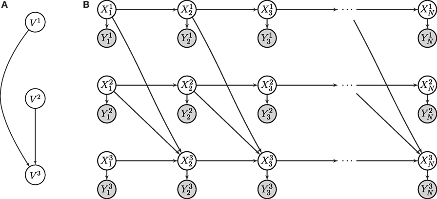
Figure 1. Representation of (A) the synchronous GDS with three vertices (V¹, V² and V³), and (B) the rolled-out DBN of the equivalent structure. Subsystem V³ is coupled to both subsystems V¹ and V² by means of the edges between latent variables $X_n^1\to X_{n+1}^3$ and $X_n^2\to X_{n+1}^3$.

In the rest of the paper, we use simplified notation, given this constrained graph structure. First, since our focus is on learning coupling between distributed systems, the superscripts refer to individual subsystems, not variables. Thus, although the 2TBN B_→is constrained such that ${\mathrm{\Pi }}_{G_{\to }}\left(Y_n^i\right)=X_n^i$, the notation $Y_n^{\mathit{ij}}$ denotes the measurement variable of the jth parent of subsystem i, e.g., in Figure 1, an arbitrary ordering of the parents gives $Y_n^{3,1}=Y_n^1$ and $Y_n^{3,2}=Y_n^2$. Second, the scoring functions for the 2TBN network B_→can be computed independently of the prior network B₁ (Friedman et al., 1998). We will assume the prior network is given, and focus on learning the 2TBN. As a result, we drop the subscript and note that all references to the network B are to the 2TBN. Since B_→is stationary, learning B_→is equivalent to learning the synchronous GDS.

5. Learning Synchronous GDSs from Data

In this section, we develop the theory for learning the synchronous update GDS from data. We will focus on techniques for learning graphical models using the score and search paradigm, the objective of which is to find a DAG G* that maximizes a score g(B : D). Given such a score, we can then employ established search procedures to find the optimal graph G*. Thus, we can state that our main goal is to derive a tractable scoring function g(B : D) for synchronous GDSs that gives a parsimonious model for describing the data.

To derive the score, we use the DBN formulation of synchronous GDSs (Sec. 4) to show that we cannot directly compute the posterior probability of the network structure (Sec. 5.1). By making some assumptions about the system, however, we are able to compute scores for GDSs by use of attractor reconstruction methods (Sec. 5.2). We conclude this section by giving an interpretation of the log-likelihood in terms of information transfer (Sec. 5.3).

5.1. Structure Learning for DBNs

Ideally, we want to be able to compute the posterior probability of the network structure G, given data D. Using Bayes’ rule, we can express this distribution as $p\left(G\mathrm{|}D\right)\propto p\left(D\mathrm{|}G\right)p\left(G\right)$, where p(G) encodes any prior assumptions we want to make about the network G. Thus, the problem becomes that of computing the likelihood of the data, given the model, p(D|G). The likelihood can be written in terms of distributions over network parameters (Friedman et al., 1998):

$p\left(D\mathrm{|}G\right)=\int p\left(D\mathrm{|}G,\mathrm{\Theta }\right)p\left(\mathrm{\Theta }|G\right)d\mathrm{\Theta },$ (8)

where we denote $\ell \left({\widehat{\Theta }}_G:D\right)=\text{log }p\left(D\mathrm{|}G,{\widehat{\Theta }}_G\right)$ as the log-likelihood function for a choice of parameters ${\widehat{\Theta }}_G$ that maximize p(D|G, Θ), given a graph G.

A common approach to compute equation (8) in closed form is by using Dirichlet priors. This leads to the BD (Bayesian–Dirichlet) score and variants (Heckerman et al., 1995; Friedman et al., 1998). However, to obtain this analytic solution, we require counts of the tuples $\left(z_n^i,{\mathrm{\pi }}_G\left(Z_n^i\right)\right)$, which involve hidden variables. We will instead use Schwarz’s (Schwarz, 1978) asymptotic approximation of the posterior distribution, which states that

$\underset{N\to \infty }{\mathit{lim}}\text{log }p\left(D\mathrm{|}G\right)\approx \ell \left({\widehat{\Theta }}_G:D\right)-\frac{\text{log }N}{2}C\left(G\right)+\mathcal{O}\left(1\right),$ (9)

where C(G) is the model dimension (i.e., number of parameters needed for the graph G (Friedman et al., 1998)) and $\mathcal{O}\left(1\right)$ is a constant bounded by the number of potential models. The approximation of the posterior [equation (9)] requires that data come from an exponential family of likelihood functions with conjugate priors over the model G, and the parameters given the model ${\mathrm{\Theta }}_G$ (Schwarz, 1978).

Akaike (1974) gives a similar criterion by approximating the KL-divergence of any model from the data. We can compute both criteria in terms of the log-likelihood function $\ell \left({\widehat{\Theta }}_G:D\right)$ and the model dimension C(G), and thus the problem can be generalized to that of deriving an information criterion for scoring the graph of the form

$g\left(B:D\right)=\ell \left({\widehat{\Theta }}_G:D\right)-f\left(N\right)\cdot C\left(G\right).$ (10)

When f (N) = 1, we have the AIC score (Akaike, 1974); f (N) = log (N)/2 yields the BIC score (Schwarz, 1978), and f (N) = 0 gives the maximum likelihood score.

5.2. Deriving the Scores for Synchronous GDSs

To calculate the information criterion [equation (10)], we require tractable expressions for the log-likelihood function $\ell \left({\widehat{\Theta }}_G:D\right)$ and the model dimension C(G). The form of the CPD in equation (7) specifies these functions, and for equation (9) to hold, this distribution must come from an exponential family (Schwarz, 1978). We do not assume the underlying model is linear-Gaussian or other known distributions, and thus express the log-likelihood as the maximum likelihood estimate for multinomial distributions (Friedman et al., 1998). From equation (7), the log-likelihood then decomposes as

$\begin{array}{l}\ell \left({\widehat{\Theta }}_G:D\right)=-N{\displaystyle \sum _{i=1}^M}{\displaystyle \sum _{x_{n+1}^i}}{\displaystyle \sum _{{\mathrm{⟨}{x}_n^{\mathit{ij}}\mathrm{⟩}}_j}}{p}_D\left(x_{n+1}^i,x_n^i,{\mathrm{⟨}{x}_n^{\mathit{ij}}\mathrm{⟩}}_j\right)\text{log }{p}_D\left(x_{n+1}^i\mathrm{|}{x}_n^i,{\mathrm{⟨}{x}_n^{\mathit{ij}}\mathrm{⟩}}_j\right)\hfill \\ -N{\displaystyle \sum _{i=1}^M}{\displaystyle \sum _{x_{n+1}^i}}{\displaystyle \sum _{y_{n+1}^i}}{p}_D\left(y_{n+1}^i,x_{n+1}^i\right)\text{log }{p}_D\left(y_{n+1}^i\mathrm{|}{x}_{n+1}^i\right)\hfill \end{array}$ (11)

Note that although we describe the states and observations as discrete in equation (11), we assume the data are generated by a continuous and stationary process. In theory, it is conceivable to have access to an infinite dataset containing realizations of all potential states and observations. In practice, we have a limited dataset and therefore must implement a discretization scheme. Modeling the dynamical systems with non-parametric techniques requires that the number of parameters scales linearly in the size of the data, and thus C(G) scales linearly with N. Instead, later, we will assume the observation data are discretized, such that there are $\mathrm{|}{Y}_n^i\mathrm{|}$ possible outcomes for an observed random variable $Y_n^i$.

The log-likelihood function [equation (11)] involves distributions over latent variables, and thus we resort to state-space (attractor) reconstruction. First, Lemma 1 shows that a future observation from a given subsystem can be predicted from a sequence of past observations. Building on this result, we present a computable formulation of the 2TBN distribution $p_{B_{\to }}$(z_n+1|z_n) via Lemma 2. We then derive a tractable form of the log-likelihood function, presented in Lemma 1. It is then shown in Theorem 2 that these lemmas allow us to compute the information criterion equation (10).

Lemma 1. Consider a synchronous GDS (G, x_n, y_n, {fⁱ}, {ψⁱ}), where the graph G is a DAG. Each subsystem state follows the dynamics $x_{n+1}^i=f^i\left(x_n^i,{\mathrm{⟨}{x}_n^{\mathit{ij}}\mathrm{⟩}}_j\right)$ and emits an observation $y_{n+1}^i={\mathrm{\psi }}^i\left(x_{n+1}^i\right)$; the subsystem observation can be estimated, for some map Gⁱ, by

$y_{n+1}^i={\mathbf{G}}^i\left(y_n^{i,\left({\mathrm{\kappa }}^i\right)},{\mathrm{⟨}{y}_n^{\mathit{ij},\left({\mathrm{\kappa }}^{\mathit{ij}}\right)}\mathrm{⟩}}_j\right).$ (12)

Proof. Consider a forced system x_n+1 = f(x_n, w_n) with forcing dynamics w_n+1 = h(w_n) and observation y_n = ψ(x_n+1). Given this type of forced system, the bundle delay embedding theorem (Stark, 1999; Stark et al., 2003) states that the delay map ${\mathbf{\Phi }}_{f,h,\mathrm{\psi }}\left({\mathit{x}}_n,{\mathit{w}}_n\right)=y_n^{\left(\mathrm{\kappa }\right)}$ is an embedding for generic f, ψ, and h. Stark (1999) proved this result in the case of forcing dynamics h that are independent of the state x.¹ For notational simplicity, we omit dependence on the noise process for the map ${\mathbf{\Phi }}_{f,h,\mathrm{\psi }}$; the noise can be considered an additional forcing system so long as υ_f is i.i.d and ${\mathrm{\upsilon }}_{\mathrm{\psi }}$ is either i.i.d or dependent on the state (Stark et al., 2003).

Given a DAG G, any ancestor of the subsystem V ⁱ is not dependent on V ⁱ. As such, the sequence

$y_n^{i,\left({\mathrm{\kappa }}^i\right)}={\mathbf{\Phi }}_{f^i,{\mathrm{⟨}{f}^{\mathit{ij}}\mathrm{⟩}}_j,{\mathrm{\psi }}^i}\left(x_n^i,{\mathrm{⟨}{x}_n^{\mathit{ij}}\mathrm{⟩}}_j\right)$ (13)

is an embedding, since ${\mathrm{⟨}{x}_n^{\mathit{ij}}\mathrm{⟩}}_j$ is independent of $x_n^i$. Let ${\mathrm{⟨}{x}_n^{\mathit{ijk}}\mathrm{⟩}}_k$ be the index-ordered set of parents of node $X_n^{\mathit{ij}}$ (which itself is the jth parent of the node $X_n^i$). Under the constraint that G is a DAG, where the state $x_{n+1}^i=f^i\left(x_n^i,{\mathrm{⟨}{x}_n^{\mathit{ij}}\mathrm{⟩}}_j\right)+{\mathrm{\upsilon }}_{f^i}$, it follows from the bundle delay embedding theorem (Stark, 1999; Stark et al., 2003) that there exists a map Fⁱ that is well defined and a diffeomorphism between observation sequences. From equation (13), we can write this map

$\begin{array}{l}{y}_{n+1}^{i,\left({\mathrm{\kappa }}^i\right)}={\mathbf{\Phi }}_{f^i,{\mathrm{⟨}{f}^{\mathit{ij}}\mathrm{⟩}}_j,{\mathrm{\psi }}^i}\left(f^i\left(x_n^i,{\mathrm{⟨}{x}_n^{\mathit{ij}}\mathrm{⟩}}_j\right),{⟨f^{\mathit{ij}}\left(x_n^{\mathit{ij}},{\mathrm{⟨}{x}_n^{\mathit{ijk}}\mathrm{⟩}}_k\right)⟩}_j\right)\hfill \\ ={\mathbf{\Phi }}_{f^i,{\mathrm{⟨}{f}^{\mathit{ij}}\mathrm{⟩}}_j,{\mathrm{\psi }}^i}\left(f^i\left({\mathbf{\Phi }}_{f^i,{⟨f^{\mathit{ij}}⟩}_j,{\psi }^i}^{-1}\left(y_n^{i,\left({\mathrm{\kappa }}^i\right)}\right),{⟨{\mathbf{\Phi }}_{f^{\mathit{ij}},{\mathrm{⟨}{f}^{\mathit{ijk}}\mathrm{⟩}}_k,{\mathrm{\psi }}^{\mathit{ij}}}^{-1}\left(y_n^{\mathit{ij},\left({\mathrm{\kappa }}^{\mathit{ij}}\right)}\right)⟩}_j\right)\right).\hfill \end{array}$ (14)

Denote the RHS of equation (14) as ${\mathbf{F}}^i\left(y_n^{i,\left({\mathrm{\kappa }}^i\right)},{\mathrm{⟨}{y}_n^{\mathit{ij},\left({\mathrm{\kappa }}^{\mathit{ij}}\right)}\mathrm{⟩}}_j\right)$; the last ${\mathrm{\kappa }}^i+{\sum }_j{\mathrm{\kappa }}^{\mathit{ij}}$ components of Fⁱ are trivial. Denote the first component as ${\mathbf{G}}^i:{\mathbb{R}}^{{\mathrm{\kappa }}^i}{\times }_j{\mathbb{R}}^{{\mathrm{\kappa }}^{\mathit{ij}}}\to \mathbb{R}$, then we arrive at equation (12).

Lemma 2. Given an observed dataset D = (y₁, y₂, …, y_N) where ${\mathit{y}}_n\in {\mathbb{R}}_M$ are generated by a directed and acyclic synchronous GDS $\left(G,{\mathit{x}}_n,{\mathit{y}}_n,\left\{f^i\right\},\left\{{\mathrm{\psi }}^i\right\}\right)$, the 2TBN distribution can be written as

${\displaystyle \prod _{i=1}^M}{p}_D\left(x_{n+1}^i\mathrm{|}{x}_n^i,{\mathrm{⟨}{x}_n^{\mathit{ij}}\mathrm{⟩}}_j\right)\cdot p_D\left(y_{n+1}^i\mathrm{|}{x}_{n+1}^i\right)=\frac{{\prod }_{i=1}^M{p}_D\left(y_{n+1}^i\mathrm{|}{y}_n^{i,\left({\mathrm{\kappa }}^i\right)},{\mathrm{⟨}{y}_n^{\mathit{ij},\left({\mathrm{\kappa }}^{\mathit{ij}}\right)}\mathrm{⟩}}_j\right)}{p_D\left(x_n\mathrm{|}\mathrm{⟨}{y}_n^{i,\left({\mathrm{\kappa }}^i\right)}\mathrm{⟩}\right)}.$ (15)

Proof. The generalized time delay embedding theorem (Deyle and Sugihara, 2011) states that, under certain technical assumptions, and given M inhomogeneous observation functions $\left\{{\mathrm{\psi }}^1,{\mathrm{\psi }}^2,\dots ,{\mathrm{\psi }}^M\right\}$, the map

${\mathbf{\Phi }}_{f,\mathrm{\psi }}\left(\mathit{x}\right)=\mathrm{⟨}{\mathbf{\Phi }}_{f^1,{\mathrm{\psi }}^1}\left(\mathit{x}\right),{\mathbf{\Phi }}_{f^2,{\mathrm{\psi }}^2}\left(\mathit{x}\right),\dots ,{\mathbf{\Phi }}_{f^M,{\mathrm{\psi }}^M}\left(\mathit{x}\right)\mathrm{⟩}$ (16)

is an embedding where each subsystem (local) map ${\mathbf{\Phi }}_{f^i,{\mathrm{\psi }}^i}:\mathcal{M}\to {\mathbb{R}}^{{\mathrm{\kappa }}^i}$, and, at time index n is described by

${\mathbf{\Phi }}_{f^i,{\mathrm{\psi }}^i}\left({\mathit{x}}_n\right)=y_n^{i,\left({\mathrm{\kappa }}^i\right)}=\mathrm{⟨}{\mathrm{\psi }}^i\left({\mathit{x}}_n\right),{\mathrm{\psi }}^i\left({\mathit{x}}_{n-{\mathrm{\tau }}^i}\right),{\mathrm{\psi }}^i\left({\mathit{x}}_{n-2{\mathrm{\tau }}^i}\right),\dots ,{\mathrm{\psi }}^i\left({\mathit{x}}_{n-\left({\mathrm{\kappa }}^i-1\right){\mathrm{\tau }}^i}\right)\mathrm{⟩}$

where ${\sum }_i{\mathrm{\kappa }}^i=2d+1$ (Deyle and Sugihara, 2011).² Therefore, the global map equation (16) is given by ${\mathbf{\Phi }}_{f,\mathrm{\psi }}\left({\mathit{x}}_n\right)=\mathrm{⟨}{y}_n^{i,\left({\mathrm{\kappa }}^i\right)}\mathrm{⟩}$ and there must exist an inverse map ${\mathit{x}}_n={\mathbf{\Phi }}_{f,\mathrm{\psi }}^{-1}\left(\mathrm{⟨}{y}_n^{i,\left({\mathrm{\kappa }}^i\right)}\mathrm{⟩}\right)$. Given Lemma 1, the existence of ${\mathbf{\Phi }}_{f,\mathrm{\psi }}^{-1}$, and since $\forall i,\left\{y_n^{i,\left({\mathrm{\kappa }}^i\right)},{\mathrm{⟨}{y}_n^{\mathit{ij},\left({\mathrm{\kappa }}^{\mathit{ij}}\right)}\mathrm{⟩}}_j\right\}\subseteq \mathrm{⟨}{y}_n^{i,\left({\mathrm{\kappa }}^i\right)}\mathrm{⟩}$, we arrive at the following equation:

$\begin{array}{l}{\displaystyle \prod _{i=1}^M}{p}_D\left(Y_{n+1}^i={\mathbf{G}}^i\left(y_n^{i,\left({\mathrm{\kappa }}^i\right)},{\mathrm{⟨}{y}_n^{\mathit{ij},\left({\mathrm{\kappa }}^{\mathit{ij}}\right)}\mathrm{⟩}}_j\right)\mathrm{|}{y}_n^{i,\left({\mathrm{\kappa }}^i\right)},{\mathrm{⟨}{y}_n^{\mathit{ij},\left({\mathrm{\kappa }}^{\mathit{ij}}\right)}\mathrm{⟩}}_j\right)\hfill \\ =p_D\left({\mathit{X}}_n={\mathbf{\Phi }}_{f,\mathrm{\psi }}^{-1}\left(\mathrm{⟨}{y}_n^{i,\left({\mathrm{\kappa }}^i\right)}\mathrm{⟩}\right)\mathrm{|}\mathrm{⟨}{y}_n^{i,\left({\mathrm{\kappa }}^i\right)}\mathrm{⟩}\right)\hfill \\ \times {\displaystyle \prod _{i=1}^M}{p}_D\left(X_{n+1}^i=f^i\left(x_n^i,{\mathrm{⟨}{x}_n^{\mathit{ij}}\mathrm{⟩}}_j\right)\mathrm{|}{x}_n^i,{\mathrm{⟨}{x}_n^{\mathit{ij}}\mathrm{⟩}}_j\right)\hfill \\ \times {\displaystyle \prod _{i=1}^M}{p}_D\left(Y_{n+1}^i={\mathrm{\psi }}^i\left(x_{n+1}^i\right)\mathrm{|}{x}_{n+1}^i\right).\hfill \end{array}$ (17)

Rearranging equation (17) gives the equality in equation (15).

Lemma 2 shows that the distributions can be reformulated by conditioning on delay vectors. The RHS of equation (15) can be used to perform inference in the 2TBN (7). The numerator is a product of local CPDs of scalar variables, and can thus be computed by either counting (for discrete variables) or density estimation (for continuous variables). The denominator is used to compute the probability that the hidden state occured, given an observed delay vector; fortunately, Casdagli et al. (1991) established methods to compute this CPDs for a variety of practical scenarios. Therefore, Lemma 2 provides a method to perform exact inference. Using this delay vector representation, we arrive at the following theorem.

Theorem 1. Consider a synchronous GDS $\left(G,{\mathit{x}}_n,{\mathit{y}}_n,\left\{f^i\right\},\left\{{\mathrm{\psi }}^i\right\}\right)$, where the graph G is a DAG. Each subsystem state follows the dynamics $x_{n+1}^i=f^i\left(x_n^i,{\mathrm{⟨}{x}_n^{\mathit{ij}}\mathrm{⟩}}_j\right)$ and generates an observation $y_{n+1}^i={\mathrm{\psi }}^i\left(x_{n+1}^i\right)$; a complete dataset is given by the sequence of observations D = (y₁, y₂, …, y_N). The log-likelihood of the data given a network structure can be computed in terms of conditional entropy:

$\ell \left({\widehat{\Theta }}_G:D\right)=N\cdot H\left({\mathit{X}}_n\mathrm{|}\mathrm{⟨}{Y}_n^{i,\left({\mathrm{\kappa }}^i\right)}\mathrm{⟩}\right)-N\cdot {\displaystyle \sum _{i=1}^M}H\left(Y_{n+1}^i\mathrm{|}{Y}_n^{i,\left({\mathrm{\kappa }}^i\right)},{\mathrm{⟨}{Y}_n^{\mathit{ij},\left({\mathrm{\kappa }}^{\mathit{ij}}\right)}\mathrm{⟩}}_j\right)$ (18)

Proof. Substituting equation (15) into equation (11) gives the log-likelihood $\ell \left({\widehat{\Theta }}_G:D\right)$ as

$\begin{array}{l}N{\displaystyle \sum _{i=1}^M}{\displaystyle \sum _{y_{n+1}^i}}{\displaystyle \sum _{y_n^{i,\left({\mathrm{\kappa }}^i\right)}}}{\displaystyle \sum _{{\mathrm{⟨}{y}_n^{\mathit{ij},\left({\mathrm{\kappa }}^{\mathit{ij}}\right)}\mathrm{⟩}}_j}}{p}_D\left(y_{n+1}^i,y_n^{i,\left({\mathrm{\kappa }}^i\right)},{\mathrm{⟨}{y}_n^{\mathit{ij},\left({\mathrm{\kappa }}^{\mathit{ij}}\right)}\mathrm{⟩}}_j\right)\times \text{log }{p}_D\left(y_{n+1}^i\mathrm{|}{y}_n^{i,\left({\mathrm{\kappa }}^i\right)},{\mathrm{⟨}{y}_n^{\mathit{ij},\left({\mathrm{\kappa }}^{\mathit{ij}}\right)}\mathrm{⟩}}_j\right)\hfill \\ -N{\displaystyle \sum _{i=1}^M}{\displaystyle \sum _{{\mathbf{x}}_n}}{\displaystyle \sum _{\mathrm{⟨}{y}_n^{i,\left({\mathrm{\kappa }}^i\right)}\mathrm{⟩}}}{p}_D\left(x_n,\mathrm{⟨}{y}_n^{i,\left({\mathrm{\kappa }}^i\right)}\mathrm{⟩}\right)\text{log }{p}_D\left(x_n\mathrm{|}\mathrm{⟨}{y}_n^{i,\left({\mathrm{\kappa }}^i\right)}\mathrm{⟩}\right).\hfill \end{array}$ (19)

In equation (19), we have removed arguments of the joint distributions that will be nullified when multiplied with the CPD. Expressing equation (19) in terms of conditional entropy [equation (3)], we arrive at equation (18).

Theorem 2. The information criterion [equation (10)] for synchronous GDS can be computed as:

$\begin{array}{l}g\left(B:D\right)=-N\cdot {\displaystyle \sum _{i=1}^M}H\left(Y_{n+1}^i\mathrm{|}{Y}_n^{i,\left({\mathrm{\kappa }}^i\right)},{\mathrm{⟨}{Y}_n^{\mathit{ij},\left({\mathrm{\kappa }}^{\mathit{ij}}\right)}\mathrm{⟩}}_j\right)\hfill \\ -f\left(N\right)\cdot {\displaystyle \sum _{i=1}^M}\left(\mathrm{|}{Y}_n^i{\mathrm{|}}^{{\mathrm{\kappa }}^i}\cdot \left(\mathrm{|}{Y}_n^i\mathrm{|}-1\right)\cdot {\displaystyle \prod _{V^p\in {\mathrm{\Pi }}_G\left(V^i\right)}}\mathrm{|}{Y}_n^p{\mathrm{|}}^{{\mathrm{\kappa }}^p}\right).\hfill \end{array}$ (20)

Proof. The distributions for the first term in equation (18) do not depend on the parents of a subsystem and thus are independent of the graph G being considered. Therefore, we have the following equation for maximum log-likelihood:

$\underset{G}{\text{max }}\ell \left({\widehat{\Theta }}_G:D\right)=\mathcal{O}\left(N\right)-N\cdot \underset{G}{\text{min}}{\displaystyle \sum _{i=1}^M}H\left(Y_{n+1}^i\mathrm{|}{Y}_n^{i,\left({\mathrm{\kappa }}^i\right)},{\mathrm{⟨}{Y}_n^{\mathit{ij},\left({\mathrm{\kappa }}^{\mathit{ij}}\right)}\mathrm{⟩}}_j\right).$ (21)

We can now compute the number of parameters needed to specify the model as (Friedman et al., 1998)

$C\left(G\right)={\displaystyle \sum _{i=1}^M}\left(\mathrm{|}{Y}_n^i{\mathrm{|}}^{{\mathrm{\kappa }}^i}\cdot \left(\mathrm{|}{Y}_n^i\mathrm{|}-1\right)\cdot {\displaystyle \prod _{V^p\in {\mathrm{\Pi }}_G\left(V^i\right)}}\mathrm{|}{Y}_n^p{\mathrm{|}}^{{\mathrm{\kappa }}^p}\right).$ (22)

Since we are searching for the graph G* = max_G g(B : D), holding N constant, we can substitute equation (21) and equation (22) into equation (10) and ignore the constant term $\mathcal{O}\left(N\right)$ in (21).

5.3. The Log-Likelihood and Information Transfer

To conclude our study of the scores, we look at the log-likelihood in the context of information transfer. First, rearranging the terms of collective transfer entropy [equation (4)], we can rewrite the log-likelihood function [equation (18)], leading to the following result.

Proposition 1. The log-likelihood function for the synchronous GDS [equation (18)] decomposes as follows:

$\ell \left({\widehat{\Theta }}_G:D\right)=N\cdot H\left({\mathit{X}}_n\mathrm{|}\mathrm{⟨}{Y}_n^{i,\left({\mathrm{\kappa }}^i\right)}\mathrm{⟩}\right)-N\cdot {\displaystyle \sum _{i=1}^M}H\left(Y_{n+1}^i\mathrm{|}{Y}_n^{i,\left({\mathrm{\kappa }}^i\right)}\right)+N\cdot {\displaystyle \sum _{i=1}^M{T}_{{\mathrm{⟨}{Y}^{\mathit{ij}}\mathrm{⟩}}_j\to Y^i}.}$ (23)

Again, the first two terms in equation (23) do not depend on the proposed graph structure, and thus maximizing log-likelihood is equivalent to maximizing collective transfer entropy. This becomes clear when we consider the log-likelihood ratio. This ratio quantifies the gain in likelihood by modeling the data D by a candidate network B instead of the empty network $B_{\varnothing }$, i.e.,

$\ell \left({\widehat{\Theta }}_G:D\right)-\ell \left({\widehat{\Theta }}_{G_{\varnothing }}:D\right)\propto \text{log }\frac{p\left(B\mathrm{|}D\right)}{p\left(B_{\varnothing }\mathrm{|}D\right)}.$

Recall that the empty DAG $G_{\varnothing }$ is one with no parents for all vertices $\forall i,{\mathrm{\Pi }}_G\left(V^i\right)={\mathrm{⟨}{Y}_n^{\mathit{ij},\left({\mathrm{\kappa }}^{\mathit{ij}}\right)}\mathrm{⟩}}_j=\varnothing$. Substituting this definition into equation (18) [or, alternatively equation (23)] gives the following result.

Proposition 2. The ratio of the log-likelihood [equation (18)] of a candidate DAG G to the empty network $G_{\varnothing }$ can be expressed as

$\ell \left({\widehat{\Theta }}_G:D\right)-\ell \left({\widehat{\Theta }}_{G_{\varnothing }}:D\right)=N\cdot {\displaystyle \sum _{i=1}^M}{T}_{{\mathrm{⟨}{Y}^{\mathit{ij}}\mathrm{⟩}}_j\to Y^i}.$

6. Discussion and Future Work

We have presented a principled method to score the structure of non-linear dynamical networks, where dynamical units are coupled via a DAG. We approached the problem by modeling the time evolution of a synchronous GDS as a DBN. We then derived the AIC and BIC scoring functions for the DBN based on time delay embedding theorems. Finally, we have shown that the log-likelihood of the synchronous GDS can be interpreted in the context of information transfer.

The representation of synchronous GDSs as DBNs allows for inference of coupling in dynamical networks and facilitates techniques for synthesis in these systems. DBNs are an expressive framework that allows representation of generic systems, as well as a numerous general purpose inference techniques that can be used for filtering, prediction, and smoothing (Friedman et al., 1998). Our representation therefore allows for probabilistic reasoning for purposes of planning and prediction in complex systems.

Theorem 2 captures an interesting parallel between learning from complete data and learning non-linear dynamical networks. If the embedding dimension κ and time delay τ are unity, then the information criterion becomes identical to learning a DBN from complete data (Friedman et al., 1998). Thus, our result could be considered a generalization of typical structure learning procedures.

The results presented here provoke new insights into the concepts of structure learning, non-linear time series analysis, and effective network analysis (Sporns et al., 2004; Park and Friston, 2013) based on information transfer (Honey et al., 2007; Lizier et al., 2011; Cliff et al., 2013, 2016). The information-theoretic interpretation of the log-likelihood has interesting consequences in the context of information dynamics and information thermodynamics of non-linear dynamical networks. The transfer entropy terms in Propositions 1 and 2 show that the optimal structure of a synchronous GDS is immediately related to the information processing of distributed computation (Lizier et al., 2008), as well as the thermodynamic costs of information transfer (Prokopenko and Lizier, 2014).

In the future, we aim to perform empirical studies to exemplify the properties of the presented scoring functions. Specifically, the empirical studies should yield insight into the effect of weak, moderate and strong coupling between dynamical units. An important concept to consider in stochastic systems is the convergence of the shadow (reconstructed) manifold to the true manifold (Sugihara et al., 2012); we have implicitly accounted for this phenomena by using CPDs in our model, however, it is important to investigate the property of convergence with different density estimation techniques. In addition, we are interested in the effect of synchrony in these networks and the relationship to previous results for dynamical systems coupled by spanning trees (Wu, 2005). We conjecture that approach used here will allow us to derive scoring functions without the assumption of multinomial observations, and thus afford the use of non-parametric density estimators. Parametric techniques, such as learning the parameters of dynamical systems (Ghahramani and Roweis, 1999; Hefny et al., 2015), could be considered in place of the posterior approximations.

Finally, the reconstruction theorems used in this paper typically make the assumption that the map (or flow) is a diffeomorphism (invertible in time). Thus, given any state, the past and future are uniquely determined and the time delay τ can be taken positive or negative. In certain cases, however, the time-reversed system is acausal, giving a map that is not time-invertible (an endomorphism). Ideally, we would aim to have methods to infer coupling for both endomorphisms and diffeomorphisms. Takens (2002) showed that if the map is an endomorphism, taking the delay vector of temporally previous observations forms an embedding. The generalized theorems in Stark (1999), Stark et al. (2003), and Deyle and Sugihara (2011), however, were established for diffeomorphisms, rather than endomorphisms; we can only conjecture that taking a delay of past observations (as we have done throughout this paper) follows for these results. Empirical studies using the measures presented in this paper would indicate whether it is an important line of inquiry to prove the generalized reconstruction theorems for endomorphisms.

Author Contributions

OC co-wrote the manuscript, derived and proved the theorems, lemmas, and propositions. MP co-wrote the manuscript, assisted with the proofs, and supervised. RF co-wrote the manuscript, assisted with the proofs, and supervised.

Conflict of Interest Statement

The authors declare that the research was conducted in the absence of any commercial or financial relationships that could be construed as a potential conflict of interest.

Acknowledgments

We would like to thank Joseph Lizier, Jürgen Jost, and Wolfram Martens for many helpful discussions, particularly in regards to embedding theory. This work was supported in part by the Australian Centre for Field Robotics; the New South Wales Government; and the Faculty of Engineering & Information Technologies, The University of Sydney, under the Faculty Research Cluster Program.

Footnotes

1. ^Stark (1999) conjectures that the theorem should generalise to functions h that are not independent of x. To the best of our knowledge, this result remains to be proven.
2. ^The original proof (Deyle and Sugihara, 2011) uses positive lags; however, the authors note that the use of negative lags also applies [and should be used in the case of endomorphisms (Takens, 2002)].

References

Akaike, H. (1974). A new look at the statistical model identification. IEEE Trans. Automat. Contr. 19, 716–723. doi:10.1109/TAC.1974.1100705

CrossRef Full Text | Google Scholar

Boccaletti, S., Latora, V., Moreno, Y., Chavez, M., and Hwang, D.-U. (2006). Complex networks: structure and dynamics. Phys. Rep. 424, 175–308. doi:10.1016/j.physrep.2005.10.009

CrossRef Full Text | Google Scholar

Bouckaert, R. R. (1994). “Properties of Bayesian belief network learning algorithms,” in Proc. of AUAI UAI (Seattle, WA), 102–109.

Google Scholar

Casdagli, M., Eubank, S., Farmer, J. D., and Gibson, J. (1991). State space reconstruction in the presence of noise. Physica D 51, 52–98. doi:10.1016/0167-2789(91)90222-U

CrossRef Full Text | Google Scholar

Chickering, D. M. (2002). Learning equivalence classes of Bayesian-network structures. J. Mach. Learn. Res. 2, 445–498.

Google Scholar

Cliff, O. M., Lizier, J. T., Wang, P., Wang, X. R., Obst, O., and Prokopenko, M. (2016). Delayed spatio-temporal interactions and coherent structure in multi-agent team dynamics. Art. Life. 23, 1–24. doi:10.1162/ARTL_a_00221

CrossRef Full Text | Google Scholar

Cliff, O. M., Lizier, J. T., Wang, X. R., Wang, P., Obst, O., and Prokopenko, M. (2013). “Towards quantifying interaction networks in a football match,” in RoboCup 2013: Robot World Cup XVII, eds S. Behnke, M. Veloso, A. Visser, and R. Xiong (Berlin, Heidelberg: Springer-Verlag), 1–13.

Google Scholar

Deyle, E. R., and Sugihara, G. (2011). Generalized theorems for nonlinear state space reconstruction. PLoS ONE 6:e18295. doi:10.1371/journal.pone.0018295

CrossRef Full Text | Google Scholar

Friedman, N., Murphy, K., and Russell, S. (1998). “Learning the structure of dynamic probabilistic networks,” in Proc. of AUAI UAI (Madison, WI), 139–147.

Google Scholar

Gan, S. K., Fitch, R., and Sukkarieh, S. (2014). Online decentralized information gathering with spatial–temporal constraints. Auton. Robots 37, 1–25. doi:10.1007/s10514-013-9369-5

CrossRef Full Text | Google Scholar

Ghahramani, Z. (1998). “Learning dynamic Bayesian networks,” in Adaptive Processing of Sequences and Data Structures, Volume 1387 of Lecture Notes in Comp. Sci, eds C. L. Giles and M. Gori (Vietri sul Mare: Springer-Verlag), 168–197.

Google Scholar

Ghahramani, Z., and Roweis, S. T. (1999). “Learning nonlinear dynamical systems using an EM algorithm,” in Advances in Neural Information Processing Systems 11, eds M. J. Kearns, S. A. Solla, and D. A. Cohn (Cambridge, MA: MIT Press), 431–437.

Google Scholar

Granger, C. W. (1969). Investigating causal relations by econometric models and cross-spectral methods. Econometrica 37, 424–438. doi:10.2307/1912791

CrossRef Full Text | Google Scholar

Gretton, A., Spirtes, P., and Tillman, R. E. (2009). “Nonlinear directed acyclic structure learning with weakly additive noise models,” in Advances in Neural Information Processing Systems, eds Y. Bengio, D. Schuurmans, J. D. Lafferty, C. K. I. Williams, and A. Culotta, Vol. 22 (Red Hook, NY: Curran Associates, Inc.), 1847–1855.

Google Scholar

Heckerman, D., Geiger, D., and Chickering, D. M. (1995). Learning Bayesian networks: the combination of knowledge and statistical data. Mach. Learn. 20, 20–197. doi:10.1023/A:1022623210503

CrossRef Full Text | Google Scholar

Hefny, A., Downey, C., and Gordon, G. J. (2015). “Supervised learning for dynamical system learning,” in Advances in Neural Information Processing Systems, eds C. Cortes, N. D. Lawrence, D. D. Lee, M. Sugiyama, and R. Garnett, Vol. 28 (Red Hook, NY: Curran Associates, Inc), 1963–1971.

Google Scholar

Honey, C. J., Kötter, R., Breakspear, M., and Sporns, O. (2007). Network structure of cerebral cortex shapes functional connectivity on multiple time scales. Proc. Natl. Acad. Sci. U.S.A 104, 10240–10245. doi:10.1073/pnas.0701519104

PubMed Abstract | CrossRef Full Text | Google Scholar

Hoyer, P. O., Janzing, D., Mooij, J. M., Peters, J., and Schölkopf, B. (2009). “Nonlinear causal discovery with additive noise models,” in Advances in Neural Information Processing Systems, eds D. Koller, D. Schuurmans, Y. Bengio, and L. Bottou, Vol. 21 (Red Hook, NY: Curran Associates, Inc.), 689–696.

Google Scholar

Kaneko, K. (1992). Overview of coupled map lattices. Chaos 2, 279–282. doi:10.1063/1.165869

CrossRef Full Text | Google Scholar

Kantz, H., and Schreiber, T. (2004). Nonlinear Time Series Analysis. eds B. Chirikov, P. Cvitanović, F. Moss, and H. Swinney. Cambridge: Cambridge University Press.

Google Scholar

Kocarev, L., and Parlitz, U. (1996). Generalized synchronization, predictability, and equivalence of unidirectionally coupled dynamical systems. Phys. Rev. Lett. 76, 1816. doi:10.1103/PhysRevLett.76.1816

CrossRef Full Text | Google Scholar

Lam, W., and Bacchus, F. (1994). Learning Bayesian belief networks: an approach based on the MDL principle. Comput. Intell. 10, 269–293. doi:10.1111/j.1467-8640.1994.tb00166.x

CrossRef Full Text | Google Scholar

Lizier, J. T., Heinzle, J., Horstmann, A., Haynes, J.-D., and Prokopenko, M. (2011). Multivariate information-theoretic measures reveal directed information structure and task relevant changes in fMRI connectivity. J. Comput. Neurosci. 30, 85–107. doi:10.1007/s10827-010-0271-2

CrossRef Full Text | Google Scholar

Lizier, J. T., Prokopenko, M., and Zomaya, A. Y. (2008). Local information transfer as a spatiotemporal filter for complex systems. Phys. Rev. E Stat. Nonlin. Soft. Matter. Phys. 77, 026110. doi:10.1103/PhysRevE.77.026110

CrossRef Full Text | Google Scholar

Lizier, J. T., Prokopenko, M., and Zomaya, A. Y. (2010). Information modification and particle collisions in distributed computation. Chaos 20, 37109–37113. doi:10.1063/1.3486801

CrossRef Full Text | Google Scholar

Lizier, J. T., and Rubinov, M. (2012). Multivariate Construction of Effective Computational Networks from Observational Data. MIS-Preprint 25/2012. Max Planck Institute for Mathematics in the Sciences.

Google Scholar

Mortveit, H. S., and Reidys, C. M. (2001). Discrete, sequential dynamical systems. Discrete Math. 226, 281–295. doi:10.1016/S0012-365X(00)00115-1

CrossRef Full Text | Google Scholar

Park, H.-J., and Friston, K. (2013). Structural and functional brain networks: from connections to cognition. Science 342, 1238411. doi:10.1126/science.1238411

CrossRef Full Text | Google Scholar

Peters, J., Janzing, D., and Schölkopf, B. (2011). Causal inference on discrete data using additive noise models. IEEE Trans. Pattern Anal. Mach. Intell. 33, 2436–2450. doi:10.1109/TPAMI.2011.71

PubMed Abstract | CrossRef Full Text | Google Scholar

Prokopenko, M., and Lizier, J. T. (2014). Transfer entropy and transient limits of computation. Sci. Rep. 4, 5394. doi:10.1038/srep05394

CrossRef Full Text | Google Scholar

Schreiber, T. (2000). Measuring information transfer. Phys. Rev. Lett. 85, 461–464. doi:10.1103/PhysRevLett.85.461

PubMed Abstract | CrossRef Full Text | Google Scholar

Schumacher, J., Wunderle, T., Fries, P., Jäkel, F., and Pipa, G. (2015). A statistical framework to infer delay and direction of information flow from measurements of complex systems. Neural Comput. 27, 1555–1608. doi:10.1162/NECO_a_00756

CrossRef Full Text | Google Scholar

Schwarz, G. (1978). Estimating the dimension of a model. Ann. Stat. 6, 461–464. doi:10.1214/aos/1176344136

CrossRef Full Text | Google Scholar

Sporns, O., Chialvo, D. R., Kaiser, M., and Hilgetag, C. C. (2004). Organization, development and function of complex brain networks. Trends Cogn. Sci. 8, 418–425. doi:10.1016/j.tics.2004.07.008

CrossRef Full Text | Google Scholar

Stark, J. (1999). Delay embeddings for forced systems. I. Deterministic forcing. J. Nonlin. Sci. 9, 255–332. doi:10.1007/s003329900072

CrossRef Full Text | Google Scholar

Stark, J., Broomhead, D. S., Davies, M. E., and Huke, J. (2003). Delay embeddings for forced systems. II. Stochastic forcing. J. Nonlin. Sci. 13, 519–577. doi:10.1007/s00332-003-0534-4

CrossRef Full Text | Google Scholar

Sugihara, G., May, R., Ye, H., Hsieh, C.-H., Deyle, E., Fogarty, M., et al. (2012). Detecting causality in complex ecosystems. Science 338, 496–500. doi:10.1126/science.1227079

PubMed Abstract | CrossRef Full Text | Google Scholar

Takens, F. (1981). “Detecting strange attractors in turbulence,” in Dynamical Systems and Turbulence, Volume 898 of Lecture Notes in Math, eds D. A. Rand and L-S. Young (Warwick: Springer-Verlag), 366–381.

Google Scholar

Takens, F. (2002). The reconstruction theorem for endomorphisms. Bull. Br. Math. Soc. 33, 231–262. doi:10.1007/s005740200012

CrossRef Full Text | Google Scholar

Umenberger, J., and Manchester, I. R. (2016). “Scalable identification of stable positive systems,” in Proc. of IEEE CDC, Las Vegas, NV.

Google Scholar

Vicente, R., Wibral, M., Lindner, M., and Pipa, G. (2011). Transfer entropy – a model-free measure of effective connectivity for the neurosciences. J. Comput. Neurosci. 30, 45–67. doi:10.1007/s10827-010-0262-3

CrossRef Full Text | Google Scholar

Wu, C. W. (2005). Synchronization in networks of nonlinear dynamical systems coupled via a directed graph. Nonlinearity 18, 1057. doi:10.1088/0951-7715/18/3/007

CrossRef Full Text | Google Scholar

Xu, Z., Fitch, R., Underwood, J. P., and Sukkarieh, S. (2013). Decentralized coordinated tracking with mixed discrete-continuous decisions. J. Field Robot. 30, 717–740. doi:10.1002/rob.21471

CrossRef Full Text | Google Scholar