Modularity and Sparsity: Evolution of Neural Net Controllers in Physically Embodied Robots

Introduction

The evolution of modularity is a central concern for biologists, neuroscientists, and roboticists alike, as modularity has been found to positively correlate with a number of desirable features of adaptive systems. These features include rapid response to environmental change (Lipson et al., 2002; Kashtan and Alon, 2005), specialization without forfeiting generally useful subfunctions (Espinosa-Soto and Wagner, 2010), avoidance of catastrophic forgetting in neural networks (Ellefsen et al., 2015), and evolvability (Wagner, 1996; Rorick and Wagner, 2011; Clune et al., 2013). To date, efforts to model and test hypotheses about the evolution of modularity have focused on using non-embodied systems to test ideas drawn from genetic regulatory networks and artificial neural networks (ANNs) (Voordeckers et al., 2015). However, some work has been dedicated to the specific challenges of evolving modularity in embodied systems (Bongard, 2011, 2015; Bernatskiy and Bongard, 2015; Bongard et al., 2015).

Contrary to the prediction that modularity evolves in response to selection on performance alone, it has been shown to evolve, instead, as a by-product of selection for enhanced performance and reduced connection costs (Clune et al., 2013). As the number of connections is reduced, the network’s sparsity increases and drives the increase in modularity. Testing the importance of initial conditions, Bernatskiy and Bongard (2015) found that modularity evolved more rapidly under selection for enhanced performance and reduced connection costs when populations were seeded with sparse networks compared to those seeded with dense networks. These computer simulations support Clune et al. (2013) hypothesis of a causal linkage between the evolution of modularity and sparsity. We call this the “modularity–sparsity hypothesis.” Because this hypothesis has only been tested in digital simulation, our aim is to test its generality by evolving neural net controllers in physically embodied robots. We predict that if an initial, randomly generated population contains some sparse networks, both modularity and sparsity will increase under selection for enhanced behavioral performance.

The networks used in this study were recurrent ANN controllers. Each ANN had two light-dependent resistors (LDRs) for inputs and two motor outputs to control the frequency and turning of a flapping propulsive tail of a swimming robot. A population of robots was created, each individual initially having a randomly generated ANN. Individuals were then subjected to artificial selection, testing their ability to detect, navigate toward, and collect energy at a light source, a behavior called phototaxis. Those individuals with better phototaxis relative to other individuals preferentially transmitted their genetic information, which represented the connections in their ANN, to the next generation.

Sparsity, S, of the ANN was measured simply as the difference between one and the ratio of actual to possible connections. Ranging from 0 to 1, higher values of S indicate fewer connections, with S = 1 meaning no connections. Since S = 1 is an impossible state for a controller that links inputs with outputs, we expect a high but non-unity level of S to provide the best controller performance.

Modularity of the controller was measured using the algorithm of Blondel et al. (2008), yielding a number, Q, from 0 to 1. When Q = 0, all possible connections among nodes are made and the network is fully integrated. The value of Q grows as connections are lost, provided that the remaining connections partition the network into groups that have nodes that are more densely connected to each other than they are to other nodes. Algorithmically, Q is determined as the difference between the fraction of connections that fall within the given groups and such fractions if the connections were distributed at random, maximized over all possible decompositions of the node set into groups. It is important to note that at a given intermediate value (0 < Q < 1), Q may correspond to many different networks.

In an ANN serving as a controller for a mobile robot, we expect a Q-mediated trade-off between the simplicity and complexity of sensorimotor control. If we imagine a high-Q controller in which two sensors are connected independently to two motors, then those two sensorimotor modules cannot combine information or calculations. Control of each module is simple, but completely separate modules cannot be coordinated by the controller. In general, larger values of Q indicate greater independence, and less interference, among the modules (Wagner and Altenberg, 1996), a feature that impacts both sensorimotor circuit function and the ability to evolve and differentiate multiple circuits within a single network.

At the other end of the spectrum, a low-Q ANN serving as a controller combines sensor inputs and shares calculations among motor output nodes. This allows for more complex patterns of operation. If the Q of the controller arises directly from the Q of the genetic regulatory network, then low Q also increases pleiotropic effects during evolution (Wagner and Altenberg, 1996). In animals, the value of Q that balances the trade-offs between simplicity and complexity of motor control likely depends on behavioral and ecological circumstances. Kim and Kaiser (2014) found Q values of 0.15 and 0.26 in the neural connectomes of the round worm, Caenorhabditis elegans, and the human, Homo sapiens, respectively.

Structural measures such as S and Q are not intended to measure the functional dynamics of the network. To examine the function of an ANN operating within a body that interacts with an environment, physically embodied robots are particularly useful, since the combined system often produces unanticipated behavior. For example, in this study we were surprised to find high variance in the behavior of our evolved robots. Upon investigation, we discovered that recurrence in the hidden layer of the ANN caused integer overflow in the calculations of those nodes. Thus the direct output to the two motor control nodes oscillated wildly, varying every few time steps across the whole range of the signed 16-bit integer. Yet the robots functioned and their behavior improved under selection for enhanced performance.

We test the Q–S hypothesis using a population of physically embodied, behaviorally autonomous, and surface-swimming robots called Tadros (tadpole robots). We selected this system for four reasons. First, this is the first time, to our knowledge, that the Q–S hypothesis has been tested in physically embodied robots. Second, Tadros are capable of helical klinotaxis (HK), a type of gradient climbing that requires only a single LDR and a single motor control variable (Long et al., 2004). This sensorimotor simplicity increases the probability, relative to more complex systems, that working behaviors will be evolved by increasing S after controller networks have been generated randomly in the starting population. Third, since the HK circuit requires a single connection from LDR to motor, this allows for multiple parallel circuit modules and hence allows Q to evolve in a system with, for example, two LDRs and two motor control variables. Fourth, we have extensive experience testing and evolving Tadros.

Previously, we evolved Tadros to test hypotheses regarding the evolutionary dynamics of morphology. Under selection for enhanced phototaxis, the tail morphology of a population of Tadros evolved (Long et al., 2006). With the addition of a predator, a second eye, and a predator-detection system, constant selection pressure on Tadros for enhanced phototaxis and predator avoidance yielded variable evolutionary patterns, a combination of directional, random, and correlated (“by-product”) effects on morphology of the flapping tail and the sensitivity of the predator-detection system (Doorly et al., 2009; Long, 2012; Roberts et al., 2014). In this study, we keep morphology constant and permit the connections of the controller to evolve under selection for enhanced phototaxis.

The framework for the controller of Tadro is a three-layer ANN with recurrence in the hidden layer (Figure 1). While the structure of each individual’s ANN may vary, 60 connections between 10 nodes are possible. The connections may have weights of −1 (inhibitory), 0 (no connection), or 1 (excitatory). At each time step, a node sums the values from the nodes that feed into it, where the value from an upstream node is the product of its connection weight and its activation. If the sum is outside of the limits of the integer type we use to represent the node state (16-bit signed), overflow occurs. Since it is a signed integer that is overflowing, the behavior is undefined. Note that the microcontroller we used is a deterministic device and in practice the resulting value is a function of the microcontroller’s state preceding the overflow.

FIGURE 1

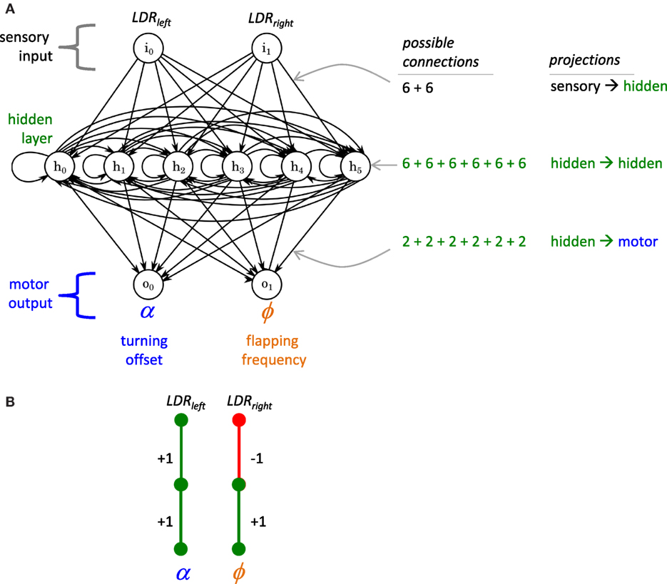
Figure 1. Framework for Tadro’s artificial neural network (ANN). (A) The basic framework is a 2 × 6 × 2 recurrent network instantiated in software. Two inputs are the light-dependent resistors (LDRs), left and right, mounted on the perimeter of the hull. Each input may have up to six connections to the nodes of the hidden layer. Each of the six nodes of the hidden layer may have up to six recurrent connections, one with itself and five with other hidden layer nodes (represented by the horizontal line connecting the nodes). The nodes of the hidden layer may have up to two connections to the nodes of the motor output layer. The weights of the connections may be −1, 0, or 1, inhibitory, missing, or excitatory, respectively. At each time step, each node sums inputs and generates a single activation. (B) Engineered network. This is the simplest network that solves the task of phototaxis in this environment using both sensors and both motor outputs. It has a modularity, Q, value of 0.5, a sparsity, S, value of 0.93 for the whole ANN, and a fitness value, ω, of 52.6 × 10⁶. Since this engineered solution represents a local optimum in the Q–S fitness landscape, we expect a starting population of randomly generated networks to evolve toward this structure.

Each of the two input nodes can make up to six connections with each of the six nodes in the hidden layer for a total of 12 possible downstream connections. Each hidden layer node can have up to six recurrent connections, one with itself (“recurrent self-connection”), and up to five with the other five nodes in the hidden layer, for up to 36 possible recurrent connections. In addition, each hidden layer node can connect to each of the two nodes of the output layer, for a maximum of 12 downstream connections. The two output nodes provide signals to the servo motor that flaps Tadro’s tail. One output node controls the tail’s flapping frequency, ϕ, while the other controls the tail’s turning offset angle, α.

According to the Q–S hypothesis, we expect that evolution by selection for enhanced phototaxis will create behaviors where the Tadro swims directly and quickly to the light and then slows down, thus maximizing energy harvested by remaining directly under the light for as long as possible. We expect that ANNs with the best phototaxic behavior would have evolved a highly modular controller with a navigational module that links the LDRs to α and a propulsion module that links the LDRs to ϕ (Figure 1B). Q and S would work in concert to keep these modules separate and thus avoid functional interference between the two. Thus the simple task of phototaxis, in conjunction with a morphological framework of two sensors and two motor outputs, is sufficient to permit the evolution of both Q and S.

Materials and Methods

Artificial Neural Network

The basic framework of the ANN was a 2 × 6 × 2 recurrent network (Figure 1). The raw data from the two LDRs fed to the input nodes were constrained to the range 0–250 by truncating values above 250. This high value was achieved when the Tadro was stationed directly under the light in the experimental pool. At the perimeter of the pool, values approached 0 if the Tadro was oriented away from the light, toward the wall. Input values were passed to hidden layer nodes via connections that would multiply the input value by −1, 0, or 1. Thus, the value of a given hidden layer node was the sum of products of the input node(s) connected to it and the connection weight linking the input node to the hidden node.

Recurrence occurred within the hidden layer. Each hidden node was updated using a sum of values from other nodes in the previous time step multiplied by the respective connection weights, −1, 0, or 1, from each of the other hidden nodes to the node being calculated. Finally, this same summing of products was performed with every hidden node connecting to a given output node. The final sum of products for a given output node was then constrained to the minimum and maximum values calculated for that node in that ANN during the program’s setup routine. This constrained value was then mapped onto the relevant ranges for the tail’s flapping frequency, ϕ, and turning offset angle, α: 1.7–5.0 Hz and 10–170°, respectively.

Software

The base code for the Tadro was implemented in C (Arduino IDE version 1.6.0) on a TinyDuino microcontroller (ASM2001, Rev.8, http://Tiny-Circuits.com). For each different individual ANN, a header file contained the 60 connection weights. Within the base code, a setup routine initiated communication with the micro SD shield so that data could be logged during the experiment, and it scaled the range of raw output values by calculating the minimum and maximum values possible for each of the two output nodes, which varied for each ANN.

The main loop of the base code consisted of four parts: (1) reading sensor pins, (2) executing the ANN, (3) recording sensor, output, and timestamp data, and (4) executing the tail-beat. Three sensor pins are read: the two navigational LDRs and the LDR “light mouth” that is centrally located on the top of the Tadro and keeps track of how much light (which is our proxy for energy) the robot harvests during a trial. The navigational LDR values become the ANN input node values. The first of the output values is mapped to the range 10–170° for α, while the second is mapped to the range 5–15 ms to calculate ϕ (see next paragraph).

The tail flap function sends a PWM (pulse-width modulated) signal to the servo motor. The range of motion of the motor is limited to ±90°, with 0° as the midline. The servo receives two inputs: α and ϕ, both of which can be adjusted once each flapping cycle. During swimming, α turns the Tadro. When the tail flaps, its amplitude is ±10° relative to the α. Hence, α is limited to ±80° relative to the midline. The flapping function sends the servo to a position of α −10° and then steps in 1° increments to α +10°. Each half-tail flap thus has 20 steps. Each step has a duration of 1/20th of half of the period, T, where T = 1/f, where f is frequency (Hz). Without a connection from the ANN to the ϕ node, the tail flaps at its maximum f, 5 Hz.

After completing data collection our analysis of logged motor output revealed that the values of the nodes within the hidden layer were overflowing. Because of the many recursive connections, the node values quickly exceeded the maximum possible for a signed 16-bit integer. At that point the output of a node began oscillating wildly.

The Tadro controllers exhibit oscillations whenever any recurrent self-connections are present (Figure 1). The probability that any ANN will lack recurrent self-connections is (1/3)⁶ = 1.4 × 10⁻³, where 1/3 is the probability of a connection weight of 0 and each of the six nodes in the hidden layer may connect to itself. Given that only 100 networks were considered in our experiment, it is unlikely that any non-oscillating networks have participated in this study. Given its likely presence, our concern was that this behavior would eliminate or substantially attenuate information passed between the sensory inputs and motor outputs.

To assess whether useful signal was reaching motors in spite of the oscillations, we investigated a pair of controllers, one randomly created and the other evolved. Individual T_0_9 was randomly created in generation 0 and had five recurrent self-connections. It had the best performance of any individual in that generation and was the most successful over the course of the evolutionary runs, leaving seven descendants in the final population. Individual T_9_9 was one of those descendants, a member of the final generation, possessing the highest fitness score of any individual over the entire evolutionary run. Like T_0_9, it also had five recurrent self-connections. We sought to understand whether the relatively high fitness of either T_0_9 or T_9_9 could reasonably be attributed to the reactivity of the controller.

We modeled the state of each node of the ANN as a random variable and measured the mutual information between pairs of these variables. We passed the values of the sensory inputs recorded during the embodied experiment through a simulator, the ANNalyzer that runs the ANN implementation used in the embodied experiments. This resulted in 1067 states of the network. For each node of the network, the full range of possible values was divided into bins and each state of the node was labeled with the number of the bin to which the state belonged. Based on the labels, we computed an estimate of the normalized mutual information using a contingency matrix as a proxy for the bivariate joint probability distribution (implementation via SciKit by Pedregosa et al., 2011). Since in the case of both T_0_9 and T_9_9 the output o₁ is disconnected from the rest of the network, we knew a priori that the mutual information between it and any other node in the network should be 0. Thus we could use the behavior of output o₁ as our baseline reference.

Hardware

Tadro (Figure 2) was constructed with a hull of a round plastic food storage container, 800 mL volume, 14.2 cm diameter on top, tapering to 12.9 cm diameter at bottom with a depth of 6.3 cm. The servo was mounted such that its center was 4.4 cm from the edge of the hull. The Delrin™ drive shaft attached to the servo was 8.0 cm long, holding under water a 5.0-cm square rigid plastic tail of 0.1 cm thickness. Mass of the Tadro was 314 g, including its 9 V battery.

FIGURE 2

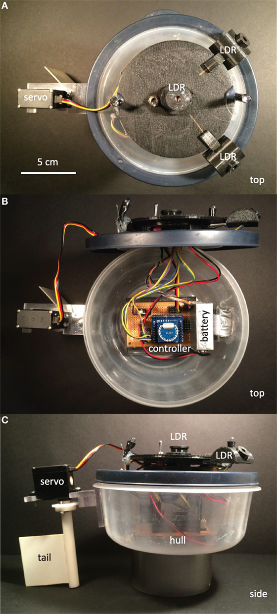
Figure 2. Tadro, mechanical design. (A) The two light-dependent resistors (LDRs) on the perimeter, angled at 45° to the horizontal, serve as inputs to the artificial neural network (ANN). The central LDR is the “light mouth,” independent of the net that logs the exposure of the Tadro to light. The servo motor drives the flapping tail. (B) The controller runs the ANN, logs sensory inputs and motor outputs, and logs light intensity from the light mouth. Power is supplied by a 9 V rechargeable lithium battery. (C) The tail is thin, rigid plastic positioned below the bottom of the hull.

The three LDRs were cadmium sulfide (model 161, http://Adafruit.com) with a resistance of approximately 200 kΩ in the dark and 10 kΩ in bright light. The servo motor was a model HS-225BB, from Hi-Tec.

Selection and Reproduction

Selection trials were run in a 3.05 m diameter indoor tank with a single light source overhead at its center (Figure 3). A gradient of light intensity was centered in the tank, with values, measured by the sensor on top of Tadro, at or near 0 near the perimeter and maximal values in the center (Figure 3B). In each generation, there were 10 genotypically unique individuals with correspondingly unique neural networks. Robots were tested one at a time in random order. Two trials were run for each individual, one starting with the LDRs toward the light and one starting with LDRs away from the light. The starting position was at the perimeter of the tank. Each trial was 5 min long.

FIGURE 3

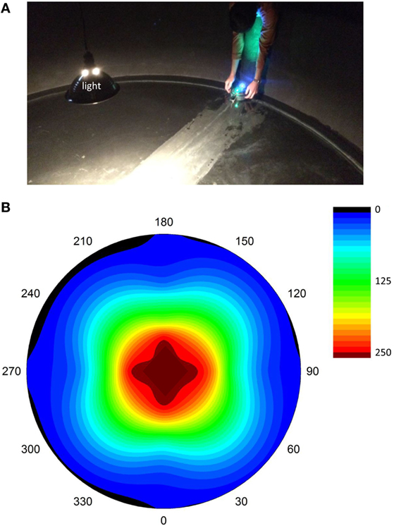
Figure 3. Selection experiments. (A) Launch of Tadro in the “head out” starting position. A single light source is present, and reflections from the walls are reduced by the black matte finish of the tank, which is 3.05 m in diameter. Each trial lasted 5 min; each of the 10 individual ANNs were tested twice (starting position head-in and head-out) in random order within that generation. (B) Light gradients in the tank, as measured by the LDR “light mouth” on the top of the Tadro. Measurements were made by manually moving the Tadro along transects running on radii from 0° to 180° and 90° to 270°. Intermediate values were interpolated between measuring points on the radii and between radii, a process that distorted the isoclines from a circular shape expected with exhaustive spatial coverage. Cool colors are low light intensity; hot colors are high light intensity. The units are arbitrary, scaled to account for the input range of the LDRs.

The proxy for the amount of energy logged in each trial was the sum of the products of the interval’s light intensity, recorded by the central LDR light mouth, and the duration of each time step. Because the light intensity values were uncalibrated, the units of energy were arbitrary but constant across individuals, trials, and generations. The energy values from both trials for an individual were averaged to calculate the individual’s fitness, ω. We calculated two variables related to changes in ω. The selection differential, d_parents, was the difference in the mean ω of the parents selected to reproduce and the mean ω of the entire parental population, including the parents. The evolutionary response, R, was the difference between the mean ω of the offspring and the mean ω of the parents.

The first generation of ANNs was created by randomly assigning values to the 60 genes in each individual. Each gene can have one of three states: −1, 0, and 1. With an equal probability of being in each state, the initial population started with an average of 40 connections per individual, where a connection is said to be present if the gene has a value of ±1.

To create the ANNs for the second and all subsequent populations, we ranked the individuals by ω. The ANN with the highest ω was cloned. The next nine offspring were produced by mutation of a parental ANN, with each parent chosen with a roulette wheel method, with the probability of reproduction proportional to their relative fitness in that generation. For each of the 60 ANN connections in each individual, the probability of mutation of any connection was 0.03 with equal probability of switching from one state to another, −1, 0, and 1.

Modularity, Sparsity, and Selection Gradients

The modularity of each ANN was quantified using the Q metric introduced by Clauset et al. (2004) and expanded by Blondel et al. (2008). The Q can be described as the difference between the fraction of connections that fall within given groups and the fraction if the same number of connections were distributed at random while preserving the nodes’ degree distribution. Quantitatively, Q is as follows:

$Q\left(\overrightarrow{c}\right)=\frac{1}{2m}{\displaystyle \sum _{i,j}}\left[A_{\mathit{ij}}-\frac{k_i{k}_j}{2m}\right]\text{δ}\left(c_i,c_j\right).$

Here, c_i denotes the label of the module to which node i is assigned, giving $\overrightarrow{c}$ the meaning of a complete assignment of the nodes into modules; A_ij is one if nodes i and j are connected and 0 otherwise; $m=\frac{1}{2}{\displaystyle \sum _{i,j}}{A}_{ij}$ is the total number of edges; $k_i={\displaystyle \sum _j}{A}_{ij}$ is the number of edges attached to the vertex i; δ(c_i, c_j) is one if nodes i and j are assigned into the same module and 0 otherwise.

The metric $Q\left(\overrightarrow{c}\right)$ depends on the assignment of nodes into modules; to obtain an assignment-independent metric we look for an assignment which maximizes the metric:

$Q=\underset{\overrightarrow{c}}{\mathit{max}}Q\left(\overrightarrow{c}\right).$

This optimization problem is computationally hard. We use an approximate optimization method by Blondel et al. (2008) to estimate Q.

Sparsity, S, of the network is measured as follows:

$S=1-\frac{C}{n},$

where C is the total number of connections with weights of ±1 and n is the total number of possible connections. For the whole ANN, n = 60 and S is indicated as S_w. The possible connections within the hidden layer, connections from the hidden layer to the α output, and connection from the hidden layer to the ϕ output, were 36, 6, and 6, respectively. The S for each is indicated as S_h, S_α, and S_ϕ.

To measure how selection is targeting traits, one may calculate selection gradients, β, the standardized coefficients from a multivariate regression of ω onto the traits:

${\text{ω}}_j=a+{\text{β}}_{Q}Q+{\text{β}}_w{S}_w+{\text{β}}_h{S}_h+{\text{β}}_{\text{α}}{S}_{\text{α}}+{\text{β}}_{\text{ϕ}}{S}_{\text{ϕ}},$

where j indexes the generation and a is a regression constant. A larger β relative to other β values indicates that that trait is a target of selection, correlated strongly with ω. We also tested the hypothesis that ω, Q, and the various types of S change over generational time using multiple one-way analyses of variance (ANOVAs), with generation as the ordinal factor and a priori effects tests to conduct pairwise generational comparisons.

Statistical Design and Analysis

This experiment was designed to test the Q–S hypothesis by testing several predictions that stem logically from it. In accordance with Fisherian statistical methods, we adopt the modus tollens logic of negation: falsifying the prediction falsifies the hypothesis. Failure to refute the predictions thus constitutes tentative support for the hypothesis.

The Q–S hypothesis (Clune et al., 2013) proposes a causal linkage between the evolution of modularity and sparsity; specifically, the evolution of S facilitates the evolution of Q, and not vice versa. Accordingly, we predict the following: S rather than Q of the ANN will be the target of selection acting on the phototactic behavior of the Tadros. In contrast to previous studies on Q and S, note that connection costs in the ANN are not part of the fitness function: ω is solely the integral of light collected by the Tadro through its “light mouth” over time (see Selection and Reproduction).

The population was evolved under selection for 10 generations, producing a total sample size of 100 individuals (10 individuals in each of 10 generations). Within the population, each individual was statistically independent; hence, ANOVA was appropriate. To test the prediction that the population would undergo adaptive evolution from its starting condition of randomly generated ANNs, we conducted a one-way ANOVA with ω as the dependent variable and generation as the independent. To test for statistical difference between generations, a priori contrasts were conducted. The identical statistical model was also used to examine the evolution of the ANN, specifically the measures of Q and S defined in the Section “Modularity, Sparsity, and Selection Gradients.” All statistical analyses were conducted using JMP software (v. 12, SAS Institute Inc., Cary, NC, USA, 1989–2016). The significance level for all tests was 0.05.

Results

Tadros with different ANNs showed differences in light-harvesting behavior (Figure 4). T_0_9 (Figure 4A) had the highest fitness, ω, in generation 0. T_0_3 (Figure 4B) had an intermediate value of ω in generation 0. T_9_9 (Figure 4C), from generation 9, had the maximum ω of any individual at any time.

FIGURE 4

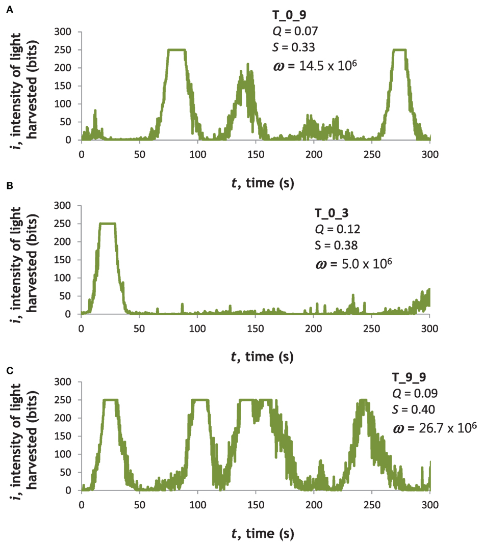
Figure 4. Light-harvesting performance varied among Tadros. Examples of three different ANNs, two (A,B) from the first generation of randomly generated ANNs (T_0_9 and T_0_3) and one (C) from the final generation (T_9_9). Naming convention: T, Tadro; first digit, generation; and second digit, rank order of individual based on fitness on ascending scale. These examples were chosen to highlight variance in the first generation and then the best individual in the last generation. Moreover, T_0_9 had the highest fitness in generation 0 and produced more descendants, including T_9_9, than any other genotype. T_0_3 had an intermediate fitness in generation 0 but produced no offspring and was selected as an example of an evolutionary dead end.

To understand the variability of an individual’s behavior, we compared the variation in ω of an individual to that of the population as a whole. We selected T_9_9 because its light-harvesting behavior was highly variable: it spent most of its time away from the wall of the tank, moving in, out, and around the light source, in a steep portion of the light gradient, as evidenced by the time-course data from the LDR “light mouth” (Figure 4C). By comparison, the behavior of individuals like T_0_3 resulted in lower fitness as a result of moving along the wall of the tank, a region with a very low level of light (Figure 4B). After the evolutionary trials, we performed 20 trials on T_9_9 (10 starting head toward the light and 10 starting head away from the light). We calculated the coefficient of variation (CV), the ratio of SD to mean, in ω, and compared that to the CV for all 20 trials (2 for each of 10 individuals) from generation 0 and generation 9. The CV values for ω were 0.738, 0.500, and 0.520, respectively.

To test whether the high variability of T_9_9 was caused by superior light-harvesting per se or the oscillatory behavior of the hidden layer of the ANN, we engineered by hand a different ANN. This engineered ANN connected the left LDR with a weight of −1 to a single hidden node; that hidden node was connected with a weight of +1 to the α output node. The right LDR with a weight of +1 was connected to a different hidden node; that hidden node was connected with a weight of +1 to the ϕ output node. Neither hidden node had connections to itself or to the other hidden node. Thus this ANN lacked recurrence and was similar to the ideal agent outlined in the Section “Introduction.” We tested the engineered ANN 20 times, 10 trials starting head toward the light and 10 starting head away from the light. It achieved a mean ω of 52.7 × 10⁶, nearly twice that of the best trial of T_9_9 (Figure 4). Its CV for ω was the lowest of all groups tested, 0.174. This was indirect evidence that recurrence in the hidden layer was creating oscillating signals that created the variability of the behavior of T_9_9.

T_0_9 left seven descendants in the final generation while T_0_3 did not reproduce (Figure 5). T_0_8 left the other three final descendants. T_9_9, a descendant of T_0_9, achieved the maximum ω of any individual in any generation. By generation 7, most individuals had evolved relatively high levels of ω.

FIGURE 5

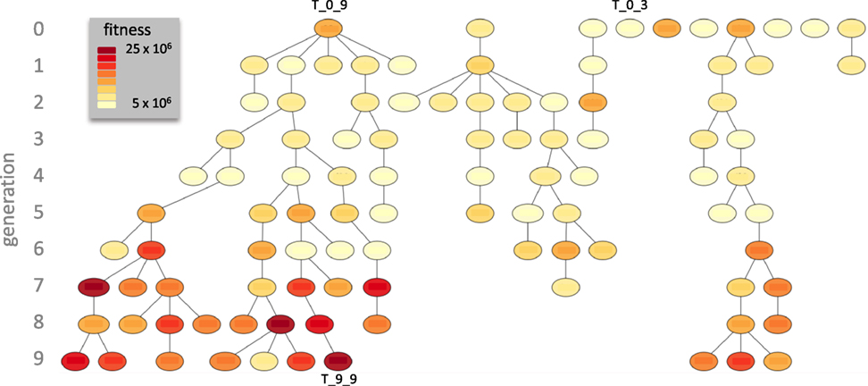
Figure 5. Descent of the Tadros. In this genealogy fitness, ω, is color coded and the three exemplar individuals (see Figure 4) are indicated. Over 10 generations of evolution, T_0_9 left the most descendants, with seven in generation 9.

On average, the population of Tadros evolved greater ω over 10 generations (Figure 6A). A strong positive directional trend (p < 0.001, ANOVA) was present. In addition to the overall trend, a priori contrasts between adjoining generations detected a significant saltation event between generations 6 and 7 (p < 0.05). The selection differential, d_parents, was always positive, but the evolutionary response, R, was not (Figure 6B). The largest values of R occurred in the transitions from generations 4 to 5 and 6 to 7.

FIGURE 6

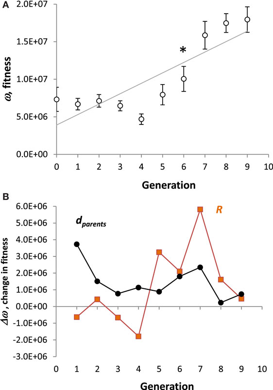
Figure 6. Evolution of Tadros. (A) Fitness. All values are means (N = 10) of the population ± SE. A strong directional trend (p < 0.001, ANOVA) is present, represented by the regression line. In spite of the overall linear trend, the pattern is more complicated: a priori contrasts between generations detect a significant saltation between generations 6 and 7 (p < 0.05, denoted by *). (B) Change in fitness. The selection differential, d_parents, is the difference in the mean fitness between parents selected to reproduce and the mean fitness of the parental population. The evolutionary response, R, is the difference between the mean fitness of the offspring and the mean fitness of the parents.

In the population of Tadros, structure of the ANN, as measured by modularity, Q, and the different types of sparsity, S, did not evolve directionally overall (Figure 7). No significant linear trends were detected by ANOVA for Q (Figure 7A), sparsity of the whole network, S_whole (Figure 7B), sparsity of the hidden layer, S_hidden (Figure 7C), sparsity of the projections to the turning offset, S_α (Figure 7D), or sparsity of the projections to the flapping frequency of the motor output layer, S_ϕ (Figure 7E). The mean S_ϕ of 0.665 was highest of the S means, which were 0.358, 0.329, and 0.390, respectively, for the others. For both the whole network and the hidden layer, a priori contrasts showed a significant saltational decrease in the mean values of S between generations 0 and 1 (p < 0.05). Over all 10 generations, the range of S_whole and Q was 0.300–0.433 and 0.016–0.133, respectively. Over 10 generations S_whole and Q were positively and significantly correlated (r = 0.407, p < 0.001).

FIGURE 7

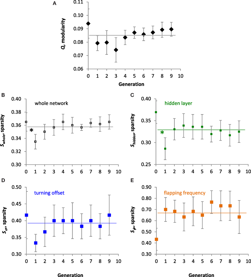
Figure 7. Evolution of the ANNs. All values are means (N = 10) of the population ± SE. (A) Modularity, Q. No significant linear trend was detected over 10 generations. The grand mean of 0.085 is indicated by the horizontal line. (B–E) Sparsity of the whole ANN, the hidden layer, projections of the hidden layer to the turning offset, and projections of the hidden layer to flapping frequency output, respectively. No significant linear trends were detected over 10 generations. Grand means of 0.358, 0.329, 0.390, and 0.665, respectively, are indicated by the horizontal lines. For both the whole network and the hidden layer, a priori contrasts showed a significant decrease in the mean values between generations 0 and 1 (*p < 0.05).

To examine the detailed correlational structure between Q and the various measures of S, we used stepwise linear regression (mixed direction, p = 0.25 to enter or leave, JMP, v. 12). Over all 100 individuals and 10 generations, S_α and S_ϕ predicted Q in the linear regression (p < 0.0001, r² = 0.293), yielding statistically significant coefficients of 0.051 (p = 0.0029) and −0.014 (p = 0.0314), respectively.

In spite of the lack of overall trends in the evolution of the structure of the ANNs, selection gradients, β, detected the effect of selection over smaller time scales. The strongest directional selection pressure acted on S_α and S_ϕ in generations 7 and 8 (Figure 8); selection switched from strongly positive to strongly negative. The switch in the sign of the selection pressure indicates stabilizing selection that can be seen most clearly for S_ϕ in the jump and plateau in magnitude over generations 6, 7, and 8 (Figure 7E). The positive selection pressure corresponded to the significant evolutionary jump in fitness from generation 6 to 7 (see Figure 6A). In no generation is Q under selection, negative or positive, that is of greater magnitude than a measure of S.

FIGURE 8

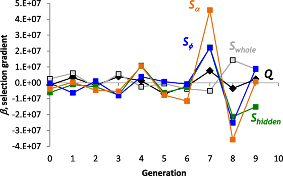
Figure 8. Selection gradients, β, for structural properties of the ANN. The largest positive and negative selection gradients occur in generation 7 and 8, respectively, for sparsity, S, of the projections from the hidden layer to offset and frequency output nodes. Linear, directional selection gradients measure the effect of each trait on fitness. Scaled coefficients allow comparisons among different properties.

The structure of the ANNs may be visualized and compared using a connectome diagram: T_0_9 and T_9_9 have an identical pattern of inputs from the sensory to the hidden layer (Figure 9); they have a nearly identical pattern of inputs to the motor layer, with only a difference in sign of one node and a complete lack of any nodes controlling the ϕ node. Contrast this pattern with that of T_0_3, which has a motor output layer dominated by connections to ϕ and has only one connection to the α node. T_0_9 and T_0_3 have a connectome similarity of 0.20, where similarity is the ratio of shared connections and weights to the total possible. T_0_9 and T_9_9, ancestor and descendent, have a connectome similarity of 0.90; T_0_3 and T_9_9 have a connectome similarity of 0.20.

FIGURE 9

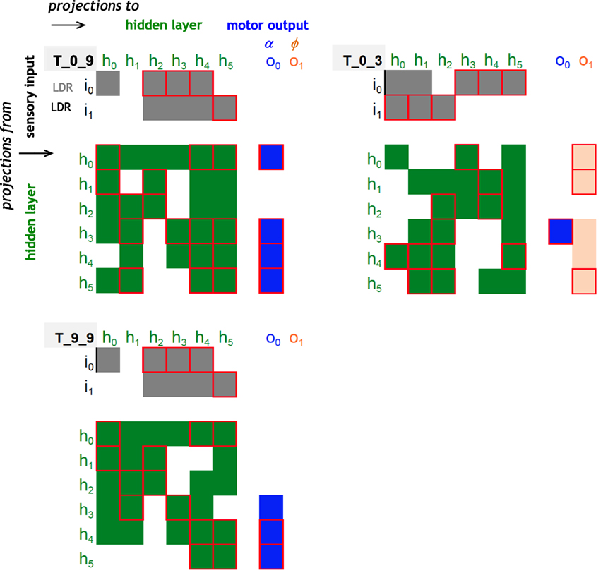
Figure 9. Connectomes of random and evolved Tadros. Same examples used in Figures 4 and 5. Projections from one node to another are indicated by the colored cells in the matrix, with positive (1) or negative (−1) connection weights with our without a red outline, respectively; lack of a connection is indicated by a blank space. Sensory projections to the hidden layer are coded in gray; hidden layer projections are coded in green when recurrent and in blue and orange for the motor output layer. T_0_9 and T_9_9 are related by descent, have an identical pattern of inputs from the sensory to the hidden layer, and have a nearly identical pattern of inputs to the motor layer, with only a difference in sign of one node and a complete lack of any nodes controlling the flapping frequency, ϕ. Contrast that pattern with the unrelated and randomly generated connectome of T_0_3.

The network structures of these individuals show clearly the differences in projections from the hidden layer to the motor output layer (Figure 10). Given the number of recurrent self-connections in the hidden layer, these networks have oscillatory behavior. Despite the oscillations, evolution by selection was able to improve the fitness of T_9_9, which has five recurrent self-connections, over that of its ancestor and the population as a whole.

FIGURE 10

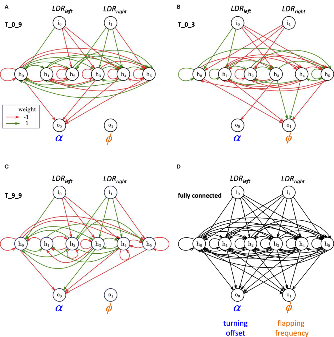
Figure 10. The structure of random and evolved ANNs, examples. (A–C) Same individuals used in Figures 4, 5 and 9. (D) A fully connected ANN for comparison.

To further probe the impact of the oscillatory behavior of the ANN, we measured the mutual information between nodes of T_9_9. First, we examined the disconnected output node o₁, that of the flapping frequency, ϕ. When paired with the input nodes, the estimates for o₁ were negative and on the order of 10⁻⁶ (Table 1). Estimates of mutual information between the inputs and the connected offset, α, output o₀ (Table 1) were found to be positive and of the order of 10⁻²–10⁻³ (Table 1). This mutual information in the connected channel, o₀, was greater than that in the disconnected one, o₁ (see also T_0_9, Table 2). The estimates of the mutual information between input and hidden neurons and between hidden neurons and the offset output neuron were of the order of 10⁻³ (Table 1; Figure 11A).

TABLE 1

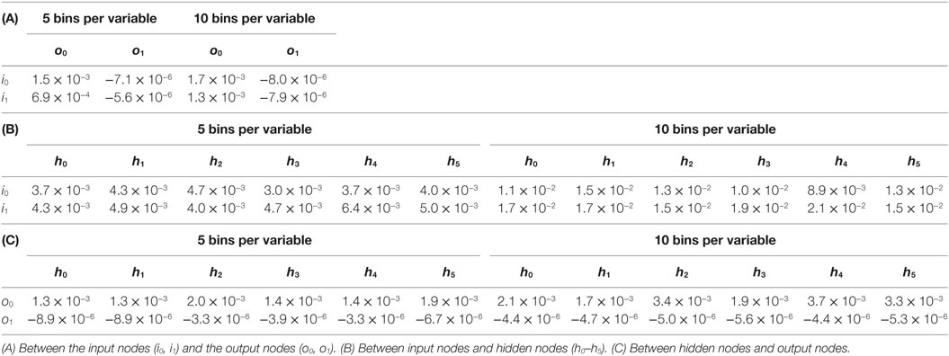
Table 1. Mutual information between the states of nodes of the ANN of T_9_9.

TABLE 2

Table 2. Mutual information between the states of nodes of the ANN of T_0_9.

FIGURE 11

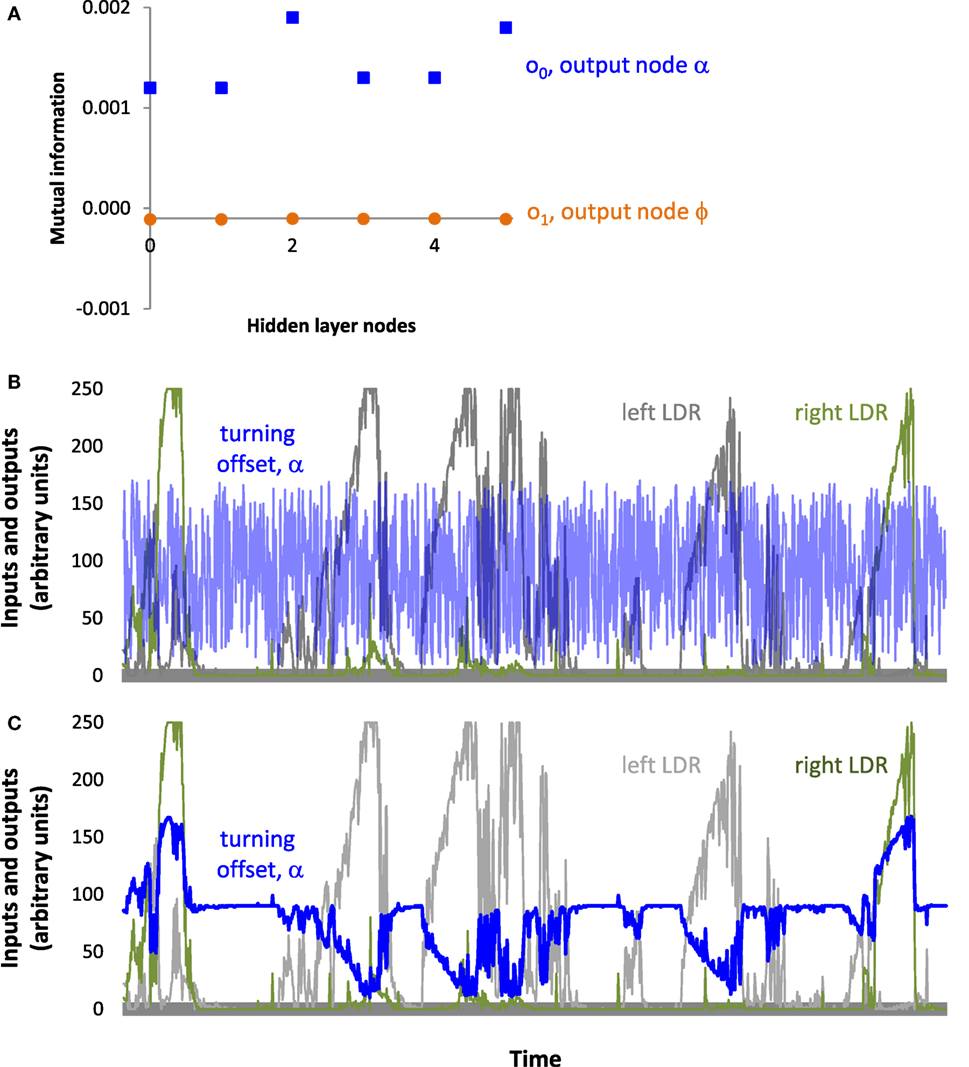
Figure 11. Information pass-through for the ANN of T_9_9. (A) Mutual information is greater in the output node, α, connected to the ANN. Since the output node for ϕ is disconnected, it serves as a reference. Note that only hidden nodes 0, 3, 4, and 5 connect directly to output node 0; the passing of information from hidden nodes 1 and 2 occurs through the other hidden nodes, to which they are connected. (B) Oscillatory output. Inputs to the two light-dependent resistors (LDRs) and the resulting output to the turning offset of the tail, α. Inputs and outputs are the actual values logged by T_9_9 during a trial. (C) Without recurrence in the hidden layer, the signals at the sensors would produce a slowly changing turning signal that would steer Tadro left and right, depending on which LDR was stimulated. These are the same inputs as above but the output is hypothetical.

These results suggest that the controller of the individual T_9_9 was indeed reactive, in spite of the variance in light-harvesting behavior and the initial impression of the oscillatory behavior of the controller (Figure 11B). Information analysis shows that output of the controller, namely the motor control, was not independent from the input, the sensor readings. Non-zero mutual information between input and hidden neurons suggests that the inputs influence the oscillating part of the network, which in turn influences the outputs. When we ran the sensory inputs logged during an experiment through our simulator (see Materials and Methods) and removed the recurrence, the controller delivered a turning signal that was tightly correlated with the inputs (Figure 11C).

Discussion

The modularity–sparsity hypothesis (Clune et al., 2013) proposes that sparsity, S, enhances the evolution of modularity, Q. We tested this hypothesis, which was based on work in digital simulation, in a population of 10 physically embodied robots, Tadros, evolved over 10 generations from a population generated randomly. When Tadros were selected for improved phototaxis, selection, as measured by linear selection gradients (Figure 8), acted to a greater degree on the S of the ANN than on Q. But S and Q were positively correlated across generations, indicating an underlying functional relationship. Thus, as predicted by the modularity–sparsity hypothesis (Clune et al., 2013), selection on S does appear to influence the evolution of Q, indirectly, in physically embodied robots.

The evolution of S and Q is complicated, even in this simple system. While the fitness, ω, of the population increases linearly over generational time (Figure 6A), S and Q do not (Figure 7). Only within a generation did we detect a strong relationship between S and ω, in the form of linear selection gradients, and then only in some generations (Figure 8). In no generation is the positive or negative magnitude of the selection gradient for Q greater than that for any aspect of S. On this evidence alone, it appears that S rather than Q is the direct target of selection in this system, as predicted from results in digital simulation (Clune et al., 2013).

As we have shown previously in Tadros (Roberts et al., 2014), phenotypes not directly targeted by selection may evolve as “by-products” yoked to targeted traits by functional correlation. Selecting for both enhanced performance and increased sparsity, Clune et al. (2013) found evidence for the by-product evolution of Q in digital simulation. This appears to be the case for Q in this population of physically embodied Tadros, as well. The S_whole and Q of all 100 of the ANNs were positively and significantly correlated (r = 0.407, p < 0.001). Moreover, when all of the metrics of S are considered at the same time, S_α and S_ϕ, are significantly correlated with Q, positively and negatively, respectively.

In addition to the difference in physical embodiment, a subtle but important difference between this paper and the simulations of Clune et al. (2013) and Bernatskiy and Bongard (2015) is that selection on Tadros resulted from a fitness function that did not explicitly represent S. This experimental approach allowed for either, both, or neither S and Q to be targeted by selection. That S emerged as a direct target and Q and an indirect by-product is thus strong evidence in support of the Q–S hypothesis.

How are S and Q related functionally? The ANN that had the highest overall fitness (T_9_9, Figure 5) appeared in the final generation, and it had a S_whole of 0.400, near the high end of the range. The relatively sparse T_9_9 controller worked to guide the robot under and in close orbit about the light source four times (Figure 4), in spite of the oscillatory behavior of its ANN (Figure 11). This effective phototaxis nearly doubled the fitness, ω, of T_9_9’s ancestor from generation 0, T_0_9, the best of that randomly generated generation. T_0_9 had a S_whole of 0.33, near the low end of the range. For this comparison, Q is less indicative of the differences in ω, with Q for T_9_9 and T_0_9 being 0.09 and 0.07, respectively.

But simple pairwise comparisons hide informative variance. For example, T_0_3 does not conform to the pattern suggested by the comparison of T_9_9 and T_0_9. Like T_0_9, T_0_3 is from the first, random generation. But it performed poorly, with a ω only one-third that of T_0_9, in spite of having an intermediate value of S_whole, 0.38, and a high value of Q, 0.12. Clearly, features of the ANN matter that are not captured in the high-level structural metrics of S_whole and Q.

The success of T_0_9 and T_9_9 may be linked, in part, to the sparsity of the projections from their ANN hidden layers to the motor output layer and the functional consequences of that pattern. Both T_0_9 and T_9_9 have 0 connections, S_ϕ = 1, from the hidden layer to the node controlling the flapping frequency, ϕ (Figures 10 and 11). On the other hand, T_0_3 has connections to both motor output nodes, the turning offset a and ϕ, with most of them to ϕ. Here is where the unintended oscillatory behavior of the hidden layer comes into play, adding noise to the motor control outputs. A simple way to reduce total noise is to eliminate one of the output channels. We have shown that a single channel can behave reactively, even with noise, as determined by mutual information analysis (Figure 11). Controlling only α, T_0_9 and most of its descendants, including T_9_9, were the most successful lineage (Figure 5). High S_ϕ at the level of projections from the hidden layer to the motor output layer improved phototaxis.

Understanding the functional importance of S_α and S_ϕ allows us to understand the evolutionary relationship between the two types of sparsity and Q. During the evolutionary jump in fitness from generation 6 to 7 (Figure 6A), the selection gradients measured in generation 7 showed strong positive selection on S_α and S_ϕ without selection on Q (Figure 7). The trend reversed in the next generation, suggesting that over those generations oscillating selection acted to stabilize these phenotypes. As selection acts directly on S_α and S_ϕ, it acts indirectly on Q because of the correlation of Q with both types of S. Interestingly, when the selection on S_α and S_ϕ is of the same sign for both, the indirect effects on Q counteract, since Q is positively and negatively correlated with S_α and S_ϕ, respectively. But since the coefficient for S_α (0.051) is approximately triple the magnitude of that for S_ϕ (−0.014), selection of the same magnitude will result in indirect selection of Q in phase with S_α.

Understanding the interactions of S, Q, and ω, we are now in a position to make predictions about the Q–S fitness landscape. Because S_whole is positively correlated with S_α (r = 0.699), we can meaningfully talk about S of the whole ANN as it relates to Q and ω. The Q–S fitness landscape contains three important landmarks (Figure 12). The first landmark is T_9_9, the best of the evolved Tadros. The second is the engineered ANN, a mobile Tadro akin to the ideal agent in this situation, with two modules (Q = 0.50), one acting to slow the tail flapping as it approaches the light and the other acting to turning more tightly as it approaches the light. The ANN of this Tadro is very simple, without recurrence in the hidden layer, and S_whole = 0.933. It also has ω nearly double that of T_9_9. But the highest possible “fitness” is actually represented by the third landmark, an immobile squatter that we simply placed directly under the light for 5 min. Lacking any connections in its ANN, the squatter has Q = 0 and S = 1. But this position in Q–S space is impossible for a Tadro to achieve, since mobile Tadros start in the dark and must move under the light. Moreover, the Tadros as built cannot stop when they get under the light, since they are programmed with a default flapping frequency. For these reasons, we predict that the population of Tadros, given sufficient time and genetic variation, would evolve up the fitness gradient that leads to the engineered Tadro.

FIGURE 12

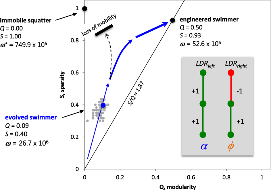
Figure 12. Predicted Q–S fitness landscape for Tadros under selection for enhanced phototaxis in a world with a single light source. While the immobile squatter has the highest light-gathering possible, the evolutionary path to that spot is blocked because of the need for mobility in the behavioral task of phototaxis. Hence, we predict that the population, given more time, will follow a path (blue arrows) toward the higher fitness of the engineered swimmer, evolving an ANN with high S_whole, intermediate Q, and no recurrence. For the experimental data (gray points), over 10 generations S_whole and Q were positively and significantly correlated (r = 0.407, p < 0.001). Inset: engineered ANN from Figure 1.

In order for this population of Tadros to climb the entire fitness gradient to the position of the engineered Tadro, one critical feature must evolve: the reduction of recurrent connections in the hidden layer. When that increase in S occurs, the population will be free to take advantage of more complex motor control by then connecting to the tail flap output. This prediction may be specific to the Tadro system with the oscillatory controllers. Were the Tadros to evolve without the oscillatory behavior, recurrence might allow for internal memory and the more complex processing and behaviors that this capacity would allow. Indeed, this possibility motivated our original decision to include recurrence in the hidden layer.

While the oscillatory behavior of the controller was an accident, it proved to be an informative one. The information from controller to motor output was sufficient to create reactive behavior, but at a cost: high variability in performance. That high variability adds noise to the relationship between selection and behavior. Thus, once recurrence is reduced by evolution, we expect evolution to accelerate. This behavior, should it occur, speaks to evolvability. The random integration of controllers, represented here by a low Q and low S in our early populations, puts brakes on evolution by spreading and propagating noise. Thus increases in Q and S are expected, up to a point, to increase mutual information between inputs and outputs. Finding systems that can autonomously evolve along complex and undulating pathways in rugged fitness landscapes continues to be a central challenge in evolutionary robotics.

Author Contributions

NL, KL, AB, MS, JS, JB, and JL conceived of and designed the experiments. NL built and programed the Tadro and ran the experiments. AB programed the reproduction and selection algorithm. MS and DW programed the neural network simulator for desktop analysis. All the authors analyzed the data and contributed to the writing of the manuscript.

Conflict of Interest Statement

The authors declare that the research was conducted in the absence of any commercial or financial relationships that could be construed as a potential conflict of interest.

Acknowledgments

The authors gratefully acknowledge the students who contributed important work to this project. Sabrina Kleman helped run the evolutionary experiments. Robot Fellows Evan Altiero, Nick Burka, John Loree, Jessica Ng, Josh Ridley, and Meghan Willcoxon helped in early robot design, prototyping, validation, and analysis of the environment and behavior. Larry Doe of Vassar College was instrumental with electronics.

Funding

This work was funded by the U.S. National Science Foundation (grant no. 1344227, INSPIRE, Special Projects).

References

Bernatskiy, A., and Bongard, J. C. (2015). “Exploiting the relationship between structural modularity and sparsity for faster network evolution,” in Proceedings of the Companion Publication of the 2015 on Genetic and Evolutionary Computation Conference (New York: ACM), 1173–1176.

Google Scholar

Blondel, V. D., Guillaume, J. L., Lambiotte, R., and Lefebvre, E. (2008). Fast unfolding of communities in large networks. J. Stat. Mech. 2008, 10008. doi:10.1088/1742-5468/2008/10/P10008

CrossRef Full Text | Google Scholar

Bongard, J. (2015). Using robots to investigate the evolution of adaptive behavior. Curr. Opin. Behav. Sci. 6, 168–173. doi:10.1016/j.cobeha.2015.11.008

CrossRef Full Text | Google Scholar

Bongard, J. C. (2011). “Spontaneous evolution of structural modularity in robot neural network controllers: artificial life/robotics/evolvable hardware,” in Proceedings of the 13th Annual Conference on Genetic and Evolutionary Computation (New York: ACM), 251–258.

Google Scholar

Bongard, J. C., Bernatskiy, A., Livingston, K., Livingston, N., Long, J., and Smith, M. (2015). “Evolving robot morphology facilitates the evolution of neural modularity and evolvability,” in Proceedings of the 2015 on Genetic and Evolutionary Computation Conference (New York: ACM), 129–136.

Google Scholar

Clauset, A., Newman, M. E., and Moore, C. (2004). Finding community structure in very large networks. Phys. Rev. E 70, 066111. doi:10.1103/PhysRevE.70.066111

PubMed Abstract | CrossRef Full Text | Google Scholar

Clune, J., Mouret, J. B., and Lipson, H. (2013). The evolutionary origins of modularity. Proc. Biol. Sci. 280, 20122863. doi:10.1098/rspb.2012.2863

PubMed Abstract | CrossRef Full Text | Google Scholar

Doorly, N., Irving, K., McArthur, G., Combie, K., Engel, V., Sakhtah, H., et al. (2009). “Biomimetic evolutionary analysis: robotically-simulated vertebrates in a predator-prey ecology,” in Artificial Life, 2009. ALife’09. IEEE Symposium (New York: IEEE), 147–154.

Google Scholar

Ellefsen, K. O., Mouret, J. B., and Clune, J. (2015). Neural modularity helps organisms evolve to learn new skills without forgetting old skills. PLoS Comput. Biol. 11:e1004128. doi:10.1371/journal.pcbi.1004128

PubMed Abstract | CrossRef Full Text | Google Scholar

Espinosa-Soto, C., and Wagner, A. (2010). Specialization can drive the evolution of modularity. PLoS Comput. Biol. 6:e1000719. doi:10.1371/journal.pcbi.1000719

PubMed Abstract | CrossRef Full Text | Google Scholar

Kashtan, N., and Alon, U. (2005). Spontaneous evolution of modularity and network motifs. Proc. Natl. Acad. Sci. U.S.A. 102, 13773–13778. doi:10.1073/pnas.0503610102

PubMed Abstract | CrossRef Full Text | Google Scholar

Kim, J. S., and Kaiser, M. (2014). From Caenorhabditis elegans to the human connectome: a specific modular organization increases metabolic, functional and developmental efficiency. Philos. Trans. R. Soc. Lond. B Biol. Sci. 369, 20130529. doi:10.1098/rstb.2013.0529

PubMed Abstract | CrossRef Full Text | Google Scholar

Lipson, H., Pollack, J. B., and Suh, N. P. (2002). On the origin of modular variation. Evolution 56, 1549–1556. doi:10.1554/0014-3820(2002)056[1549:OTOOMV]2.0.CO;2

PubMed Abstract | CrossRef Full Text | Google Scholar

Long, J. (2012). Darwin’s Devices: What Evolving Robots Can Teach Us About the History of Life and the Future of Technology. New York: Basic Books.

Google Scholar

Long, J. H. Jr., Koob, T. J., Irving, K., Combie, K., Engel, V., Livingston, N., et al. (2006). Biomimetic evolutionary analysis: testing the adaptive value of vertebrate tail stiffness in autonomous swimming robots. J. Exp. Biol. 209, 4732–4746. doi:10.1242/jeb.02559

PubMed Abstract | CrossRef Full Text | Google Scholar

Long, J. H. Jr., Lammert, A. C., Pell, C. A., Kemp, M., Strother, J. A., Crenshaw, H. C., et al. (2004). A navigational primitive: biorobotic implementation of cycloptic helical klinotaxis in planar motion. J. IEEE Oceanic Eng. 29, 795–806. doi:10.1109/JOE.2004.833233

CrossRef Full Text | Google Scholar

Pedregosa, F., Varoquaux, G., Gramfort, A., Michel, V., Thirion, B., Grisel, O., et al. (2011). Scikit-learn: machine learning in Python. J. Mach. Learn. Res. 12, 2825–2830.

Google Scholar

Roberts, S. F., Hirokawa, J., Rosenblum, H. G., Sakhtah, H., Gutierrez, A. A., Porter, M. E., et al. (2014). Testing biological hypotheses with embodied robots: adaptations, accidents, and by-products in the evolution of vertebrates. Front. Rob. AI 1:12. doi:10.3389/frobt.2014.00012

CrossRef Full Text | Google Scholar

Rorick, M. M., and Wagner, G. P. (2011). Protein structural modularity and robustness are associated with evolvability. Genome Biol. Evol. 3, 456–475. doi:10.1093/gbe/evr046

PubMed Abstract | CrossRef Full Text | Google Scholar

Voordeckers, K., Pougach, K., and Verstrepen, K. J. (2015). How do regulatory networks evolve and expand throughout evolution? Curr. Opin. Biotechnol. 34, 180–188. doi:10.1016/j.copbio.2015.02.001

PubMed Abstract | CrossRef Full Text | Google Scholar

Wagner, G. P. (1996). Homologues, natural kinds and the evolution of modularity. Am. Zool. 36, 36–43. doi:10.1093/icb/36.1.36

CrossRef Full Text | Google Scholar

Wagner, G. P., and Altenberg, L. (1996). Perspective: complex adaptations and the evolution of evolvability. Evolution 50, 967–976. doi:10.2307/2410639

CrossRef Full Text | Google Scholar