Unvealing the Principal Modes of Human Upper Limb Movements through Functional Analysis

1. Introduction

Human hands represent an extraordinary tool to explore and interact with the external environment. Not surprisingly, a lot of studies have been devoted to model how the nervous system can cope with the complexity of hand sensory-motor architecture (Mason et al., 2001; Todorov and Ghahramani, 2004; Zatsiorsky and Latash, 2004; Thakur et al., 2008; Gabiccini et al., 2013; Santello, 2014). These studies have led to the definition of the so-called synergies, broadly intended as covariation patterns that can be represented at different levels (Santello et al., 2016). More specifically, at the level of motor units, neural activation shows a synergistic control in the time and/or frequency domain (Santello, 2014). At the muscle level, different works explored patterns of muscle activity whose timing and/or amplitude modulation enables the generation of different movements, see d’Avella and Lacquaniti (2013) for a review. Synergies have also been identified and defined as covariation patterns of joint angles, e.g., hand postural synergies (Santello et al., 1998, 2013; Mason et al., 2001), or covariation patterns among digit forces [for a review see Zatsiorsky and Latash (2004)]. However, to correctly understand human manipulation, in addition to hand analysis, the role of whole upper limb movements should be also taken into account. Indeed, the whole upper limb motions are devoted to guide and optimize position and orientation of the hand w.r.t. external targets.

For these reasons, in addition to many works devoted to analyze hand behavior, it is also possible to find studies modeling human upper limb motor workspace, either from a kinematic point of view, or from a muscular or neural point of view. In Heidari et al. (2016), the authors studied the kinematic movements of upper limb during selected tasks in order to compare stroke patients and normal subjects. In Butler et al. (2010), the authors developed a quantitative method to assess upper limb motor deficits in children with cerebral palsy using three-dimensional motion analysis during the reach and grasp cycle. Other papers studied muscular synergies in upper limb activities, as in d’Avella and Tresch (2002), where the authors introduced a model based on combinations of muscle time-varying synergies, and in d’Avella et al. (2006), where authors recorded electromyographic activity from shoulder and arm muscles during point-to-point movements. As for hand synergies, whose robotic applications are reviewed in Santello et al. (2016), synergies have also been applied to movement generation for virtual arms (Fu et al., 2013) as well as myocontrol of a multi-DoF planar robotic arm using muscle synergies (Lunardini et al., 2015). However, none of the previous studies considered the dynamic aspects of human upper limb motion, i.e., that different temporal evolutions and shapes of upper limb joints trajectories would result in different final hand poses.

Typical approaches based on principal component analysis are not suitable in this case because of the underlying hypothesis of temporal uncorrelation of upper limb poses in time. For this reason, to achieve this goal, we propose to use for the fist time functional principal component analysis (fPCA) to study upper limb motions. fPCA is a statistical method for investigating dominant modes of variation of functional data in time and has been widely used in one-dimensional or multi-dimensional time series analysis in chemistry, weather phenomena, and medicine (Aguilera et al., 1999; Gokulakrishnan et al., 2006; Dai et al., 2013). The interested reader in functional data analysis could refer to Ramsay and Silverman (2002), Ramsay (2006), and Ramsay et al. (2009). In human movement studies, this method has been used to explore the presence of variations in repetitions of a specific task, e.g., in Ryan et al. (2006), an analysis of knee joint kinematics in the vertical jump was performed. In Coffey et al. (2011), fPCA was used to analyze a bio-mechanical dataset examining the mechanisms of chronic Achilles tendon injury and the functional effects of orthoses by comparing injured and healthy subjects. In Dai et al. (2013), fPCA was used in conjunction with PCA for the analysis of grasping motion. In this work, a new analysis of upper limb movements by fPCA is proposed to provide a description of the kinematic trajectories as combination of functional principal components (fPCs).

The choice to use fPCA as main data analysis tool is motivated by the fact that it allows to include some important features of the signal, such as shape and time dependence, which cannot be taken into account by other simpler data dimensionality reduction techniques (e.g., principal component analysis). To achieve this goal, we propose an experimental setup for studying upper limb movements, based on a Motion Capture (MoCap) system (Phase Space^®). Using this tool, we carried out a series of experiments with human considering a comprehensive dataset of daily living activities (ADLs) and grasping/manipulation actions. These actions were selected relying on the study of grasping taxonomies (Cutkosky, 1989; Feix et al., 2016), and considerations on human upper limb movement workspace (Lenarcic and Umek, 1994; Abdel-Malek et al., 2004; Perry et al., 2007). Our analysis has led to the reduction of complexity of upper limb trajectories by describing these as linear combinations of few principal functions (or modes). Implications for robotics are also discussed.

2. Experimental Protocol and Setup

2.1. A Set of Daily Living Tasks

In order to develop a comprehensive study of human upper limb movements, one of the key features for the generation of a valid dataset is the definition of a set of meaningful actions (Santello et al., 1998; Mason et al., 2001; Todorov and Ghahramani, 2004; Vinjamuri et al., 2010). For this reason, we selected a set of movements driven by the study of grasping taxonomies (Cutkosky, 1989; Feix et al., 2016), and the analysis of human upper limb movement workspace (Lenarcic and Umek, 1994; Abdel-Malek et al., 2004; Perry et al., 2007). The output of this selection resulted in a set of 30 different actions, divided into intransitive, transitive, and tool-mediated actions to avoid bias due to the affordances of the objects used for the grasp investigation. Indeed, as Cubelli et al. (2000) suggested starting from apraxia investigation and Handjaras et al. (2015) confirmed with cortical imaging, different movements are generated by different cortical activations, because require different motor schema, based on the type of interaction with the environment. These movements can be classified into three classes, according to the presence or absence of an object and, if the object is present, on the approach with it: intransitive class, which collects actions that does not need the use of an object; transitive class, which collects actions that introduces the use of an object; and tool-mediated class, which collects actions where an object is used to interact with another one. Tasks are meant to be executed three times with dominant hand, the subject seating on a chair, with the objects placed on a frontal table at a fixed distance. At the end of the task, the subject returned to the starting point. The complete list of actions is reported in Table 1.

TABLE 1

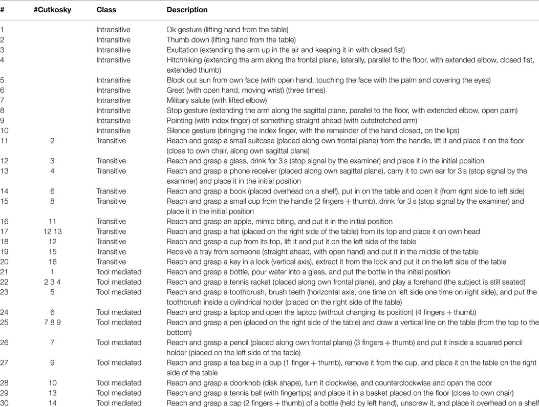
Table 1. Protocol actions.

2.2. An Experimental Setup for Data Acquisition

We focused on kinematic recordings, which were achieved using a commercial system for 3D motion tracking with active markers (Phase Space^®). Ten stereo-cameras working at 480 Hz tracked 3D position of markers, which were fastened to supports rigidly attached to upper limb links. In this manner, 20 markers were accommodated on the upper limb so that the distance between elements of each support was fixed. Supports were suitably designed for these experiments and printed in ABS (see Figure 1A). The acquisition was implemented through a custom application developed in C++, employing Boost libraries (Schäling, 2011) to enable the synchronization between Phase Space data and other sensing modalities, such as force/torque sensors and EEG, and the Phase Space OWL library to get the optical tracking system data.

FIGURE 1

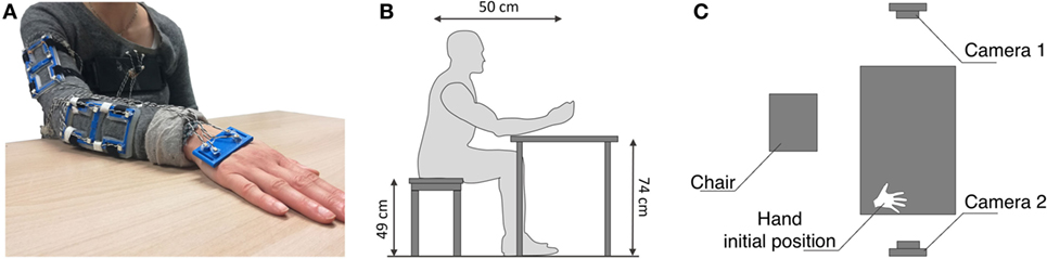
Figure 1. In these figures, we show the experimental setup. In (A) markers accommodation is shown. In (B) and (C), we report a scheme of the experimental setup. The subjects were comfortably sit in front of the table. In the starting position, the subject’s hand was located at the right side of the table. Two cameras are included to record the scene.

Seven adult right-handed subjects (5 males and 2 females, aged between 20 and 30) performed the experiment. Each task was repeated three times in order to increase the robustness of collected data. The experimenter gave the starting signal to subjects. In the instructions, the experimenter emphasized that the whole movement should be performed in a natural fashion. The object order was randomized for every subject. Each subject performed the whole experiment in a single day. No subject knew the purpose of the study, and had no history of neuromuscular disorders. Each participant signed an informed consent to participate in the experiment, and the experimental protocol was approved by the Institutional Review Board of University of Pisa, in accordance with the declaration of Helsinki. The complete experimental setup is reported in Figures 1B,C. Moreover, we used two cameras (Logitech hd 1080p) to record the scene of the experiments in order to visually compare the real and the reconstructed movement.

3. Motion Identification

3.1. Modeling of Upper Limb Kinematics

An accurate description of human upper limb is challenging due to the high complexity of the kinematic structure, e.g., for axis location and direction, which are usually time varying. In order to explore the system complexity, the interested reader can refer to Maurel and Thalmann (2000) and Holzbaur et al. (2005). In this work, we used a trade-off between complexity and accuracy taking inspiration from Benati et al. (1980). This allows to get an acceptable computational time, still maintaining a good level of explanation of physical behavior. Taking inspiration from Gabiccini et al. (2013), we adopted a model with 7 degrees of freedom (DoFs) and 3 invariable shape links. Joints angles are defined as q₁, …, q₇: q₁ is associated with the shoulder abduction–adduction; q₂ is associated with the shoulder flexion–extension; q₃ is associated with the shoulder external–internal rotation; q₄ is associated with the elbow flexion–extension; q₅ is associated with the elbow pronation–supination; q₆ is associated with the wrist abduction–adduction; q₇ is associated with the wrist flexion–extension. In Figure 2A, a scheme of the model is reported.

FIGURE 2

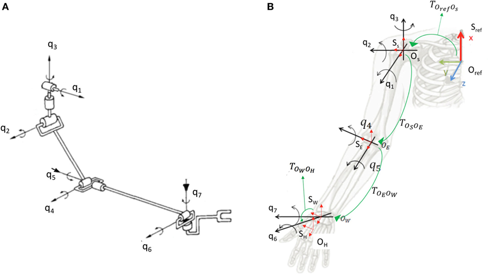
Figure 2. System parametrization. In (A), we show the kinematic model used in this work. In (B), we report the kinematic parametrization. The labels q₁, …, q₇ refers to joints of the model. S_ref refers to the reference system centered in O_ref, fixed to the epigastrium; S_S refers to the reference system centered in O_S, center of rotation (CoR) of shoulder joints, fixed to the arm; S_E refers to the reference system centered in O_E, CoR of elbow joints, fixed to the forearm; S_W refers to the reference system centered in O_W, CoR of wrist joints, fixed to the hand; S_H refers to the reference system centered in O_H, fixed to the hand. The label $T_{O_{\mathit{ref}}{O}_S}$ refers to the rigid transform between S_ref and S_S; $T_{O_S{O}_E}$ refers to the rigid transform between S_S and S_E; $T_{O_E{O}_W}$ refers to the rigid transform between S_E and S_W; $T_{O_W{O}_H}$ refers to the rigid transform between S_W and S_H.

3.2. Model Parameters

In order to describe the forward kinematics of the arm, 5 different reference systems was defined: S_ref, centered in O_ref, fixed to the epigastrium; S_S, centered in O_S, Center of Rotation (CoR) of shoulder joints, fixed to the arm; S_E, centered in O_E, CoR of elbow joints, fixed to the forearm; S_W, centered in O_W, CoR of wrist joints, fixed to the hand; S_H, centered in O_H, fixed to the hand. The rigid transform between S_ref and S_S is $T_{O_{\mathit{ref}}{O}_S}$; the rigid transform between S_S and S_E is $T_{O_S{O}_E}$; the rigid transform between S_E and S_W is $T_{O_E{O}_W}$; the rigid transform between S_W and S_H is $T_{O_W{O}_H}$. The defined reference systems are shown in red in Figure 2B. Green arrows indicate rigid transforms from a reference system and the next one in the kinematic chain. To parameterize the i-th segment, we use the product of exponentials (POE) formula (Brockett, 1984):

$g_{O_{\mathit{ref}}{O}_j}\left(\mathrm{\theta }\right)=\left[{\displaystyle \prod _{k=1}^j}{e}^{{\widehat{\mathrm{\xi }}}_k{\mathrm{\theta }}_k}\right]g_{O_{\mathit{ref}}{O}_j}\left(0\right)$

where ${\widehat{\mathrm{\xi }}}_k$ are the twists of the joints defining the kinematic chain, θ = [θ₁, …, θ_k, …, θ_j]^T are the exponential coordinates of the second kind for a local representation of SE(3) (Special Euclidean group, 4 × 4 rototranslation matrices) for the j-th link, and $g_{O_{\mathrm{ref}}{O}_j}\left(0\right)$ is the initial configuration. For further details, the interested reader can refer to Gabiccini et al. (2013).

3.3. Markers Modeling

Links movements were tracked by fastening optical active markers to upper limb links. Markers positioning is inspired by Biryukova et al. (2000). In order to improve tracking performance, a redundant configuration of marker was used, in particular 4 markers fixed to the chest, 6 markers fixed to the lateral arm, 6 markers fixed to the dorsal forearm, and 4 markers fixed to the hand dorsum. A picture showing marker distribution is reported in Figure 1A. The position of each marker can be calculated as rigid transform w.r.t. the center of the corresponding support. The supports kinematic can be described as a rigid transform from the link reference system to the support reference system, as depicted in Figure 3.

FIGURE 3

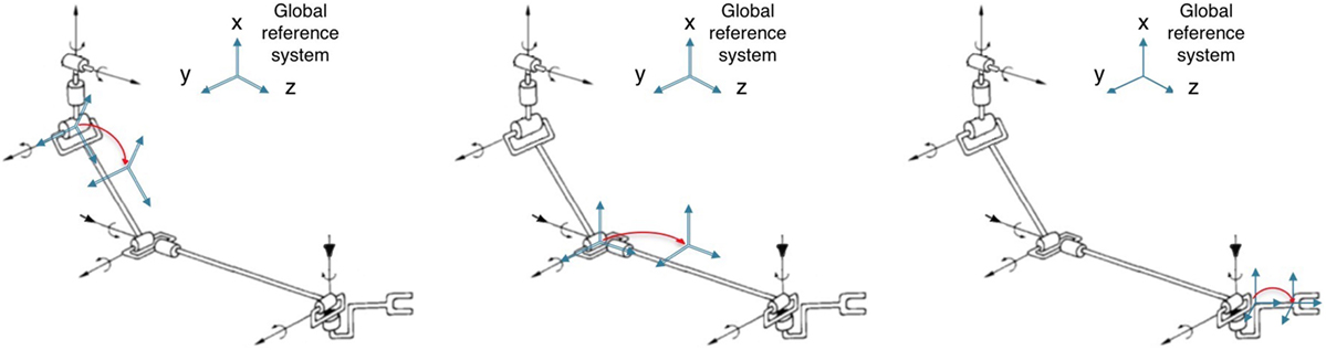
Figure 3. Markers positioning. In the left figure, we report the arm markers position; in the central figure, we report the forearm markers position; and in the right figure, we report the hand marker position.

The model is completely parameterized using 14 parameters (different for each subject) collected in a vector p_G: bones length (arm and forearm, 2 parameters); rigid transform from epigastrium to the shoulder CoR (3 parameters); rigid transform from shoulder CoR to the center of arm marker support (3 parameters); rigid transform from elbow CoR to the center of forearm marker support (3 parameters); and rigid transform from wrist CoR to the center of hand marker support (3 parameters). The parameter vector p_G was calibrated for each subject. Given p_G, the upper limb pose is described by 7 joints angles [q₁, …, q₇]^T collected in a vector x.

3.4. Model Calibration and Angles Estimation

As previously mentioned, the parameters of the kinematic model must be adapted for the specific subject that performs the experiments. The optimal parameters were obtained by solving a constrained least-squares minimization problem:

$\left(x^{\ast },p_G^{\ast }\right)=\mathit{arg}\underset{x_k\in D_x,p_G\in D_p}{\text{min}}\frac{1}{2}{\displaystyle \sum _{k=1}^{N_p}}{r}_k^T{r}_k.$

The residual function r_k is calculated as r_k(x_k, p_G): = y_k− f (x_k, p_G), where: y_k is the marker position vector measured with Phase Space; x_k is the vector of estimated joint angles; p_G is the vector of model kinematic parameters; D_x is the upper limb joints range of motion; D_p is the variation around a preliminary estimation of parameters performed with manual measurements; and f (x_k, p_G) is the estimated positions vector of markers using the forward kinematics. The vector of measures y_k and the vectors of estimations f (x_k, p_G) can be obtained by concatenating the measures of marker positions and estimations at different time frames. To obtain an effective calibration output, the selected frames for the calibration procedure must consider different poses of the kinematic chain. For the experiments reported in this work, we had r_k normalized w.r.t. the dimension of y_k equal to 15.30 ± 16.25 mm; as an example we show in Figure 4 the values of r_k in a sample task. Taking inspiration from Gabiccini et al. (2013), the calibrated model was then used to identify the joints angles using an Extended Kalman Filter (EKF). Indeed, the model can be considered as an uncertain noisy process where at time frame k the joints angle vector x_k is the state of the process, y_k is the markers position vector, w_k and v_k are process and observation zero mean Gaussian noises, with covariance Q_k and R_k, respectively, and f (x_k) is the forward kinematics. The system can be described using the following equations:

$\left\{\begin{array}{c}{x}_k=x_{k-1}+w_k\hfill \\ y_k=f\left(x_k\right)+v_k\hfill \end{array}\right..$ (1)

FIGURE 4

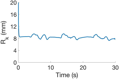
Figure 4. Mean squared error obtained in the estimation procedure in a sample. Initial error value is 57.1 mm, related to the filter initialization.

Given the state at time frame k−1, the state at time k was obtained using a 2-steps procedure: prediction of the future state ${\widehat{x}}_{k|k-1}={\widehat{x}}_{k-1}$; update of the state estimated in the first step by calculating ${\widehat{x}}_{k|k}={\widehat{x}}_{k|k-1}+K_k{\tilde{r}}_k$. The correction amount of the state prediction is the product between the residual values vector ${\tilde{r}}_k=y_k-f\left({\widehat{x}}_{k|k-1}\right)$ and the Kalman Gain K_k. This gain is calculated as product between the covariance matrix estimation of the predicted state $P_{k|k-1}$, the jacobian matrix, i.e., $H_k=\frac{\partial \left(f\left(x\right)\right)}{\partial \left(x\right)}$, and the inverse matrix of the residual covariance.

3.5. Experimental Results

The performance of the estimation tool for time frame k can be evaluated by calculating the mean squared error (MSE) R_k as

$R_k=\frac{1}{N_{\mathit{markers}}}||\left(y_k-f\left({\widehat{x}}_{k|k}\right)\right)||$

where N_markers is the number of markers, y_k is the marker positions vector, and $f\left({\widehat{x}}_{k|k}\right)$ is the vector of markers estimated positions using the joint angles calculated with the EKF. Typical values of R_k are ≈ 1 cm, with a mean error for hand and forearm markers of ≈0.5 cm and a mean error for arm markers of ≈1.8 cm. Identified angles was used to reconstruct the movements, which were represented using a virtual model of upper limb suitably implemented in MatLab for these reconstructions. The reconstructions were used for a visual check w.r.t. the real movement recorded with cameras. This allows to verify the human-likeliness of the reconstructed movement.

4. Data Analysis

The goal of this work is the study of functional motor synergies of upper limb. This is accomplished using functional PCA, a statistical method that allows to study the differences in shapes between functions. In order to avoid the inclusion in this analysis of undesired features due to misalignments in time or in velocity of the samples, we performed the following pre-processing techniques: segmentation, to divide the repetition of each task, time warping, to synchronize in time all the elements of the dataset.

4.1. Segmentation

For each task, the three repetitions have been segmented using the following procedure (see Figure 5):

1. select the data elements of the third DoF (q₃);

2. find the first two peaks p₁, p₂ of the signal;

3. evaluate the mean slope s₁, s₂ of the signal in a section close to each peak;

4. calculate the segmentation point as $t_1=\frac{p_1{s}_1+p_2{s}_2}{s_1+s_2}$;

5. repeat points 2–4 using the second and the third peaks and obtain t₂.

FIGURE 5

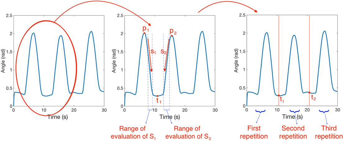
Figure 5. Segmentation procedure. In the left figure, we report a sample of joint evolution in time. In the central figure, we show two peaks of the signal p₁, p₂ and the mean slope of the signal s₁, s₂ evaluated in two ranges close to each peak. The segmentation point t₁ is evaluated as $t_{\text{1}}=\frac{p_{\text{1}}{s}_{\text{1}}+p_{\text{2}}{s}_{\text{2}}}{s_{\text{1}}+s_{\text{2}}}$. The same procedure is repeated using the second and the third peaks of the signal and the output of the segmentation procedure is reported in the right figure.

q₃ data (i.e., shoulder flexion–extension) was used for segmentation because it almost always contains three distinct peaks. If the peaks were not detectable, another DoF with detectable peaks was used instead. Note that the segmentation is performed using the same couple of segmentation points for all the 7 DoFs.

Considering different subjects and tasks, differences between shapes are evident (see Figure 6A). The three repetitions of each task should be replaced by the corresponding mean vector to increase robustness. This replacement can be performed only after signal synchronization, achieved using a time-warping procedure.

FIGURE 6

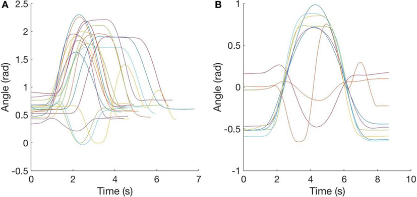
Figure 6. Segmentation and time warping. (A) Segmented data: in this plot, a sample of segmented data is reported to show the differences in starting-time and speed of the action. (B) Time-warped data: in this plot, the sample of data is shown after time warping and replacement of the three repetitions with the mean signal.

4.2. Time Warping

The synchronization between two signals allows to increase the affinity by conforming starting-time and speed of the action. This can be achieved by finding the optimal time-shift and time-stretch of one signal w.r.t. the other one. This problem is known in literature as dynamic time warping (DTW) and widely explored in sound engineering and pattern recognition (Rabiner et al., 1978; Berndt and Clifford, 1994; Müller, 2007; Salvador and Chan, 2007). In this work, DTW is needed to allow the mediation of the three repetitions, to avoid misalignment, and to compare different tasks and subjects’ data. For the problem explored in this work, the following assumptions were done: monotonicity, to preserve data integrity, and linear distortion of time. Given two time series, v₁ and v₂, the affinity between the two signals is increased by the solution of the following least-squares minimization problem:

$\left(S,T\right)=\mathit{arg}\underset{S>0,T}{\text{min}}\left(||v_1\left(t\right)-v_2\left(\mathit{St}-T\right)||\right)$

where S is a scaling factor for the velocity of signal v₂ and T is the amount of shifting in time applied to v₂. The dataset elements were time-warped w.r.t. a reference time series, selected in the set as the element whose length is the mean value w.r.t. the length of all dataset elements. For each element, S and T are calculated by performing DTW on DoFs used for segmentation, then all the components are time-warped using the optimum set of parameters. The time-warped vectors have the same number of frames (number of elements). Once the time warping was performed on all the dataset elements, the three repetitions for each task can be replaced by the corresponding mean vector. A sample output of this procedure is reported in Figure 6B. In Figure 7, a scheme of the data analysis procedure is reported.

FIGURE 7

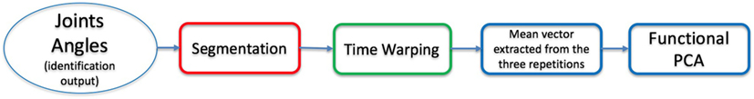
Figure 7. Scheme of data analysis.

4.3. Principal Component Analysis

To explain fPCA, it is useful to start from classic principal component analysis (PCA). Principal component analysis (PCA) is a statistical procedure that uses an orthogonal transformation to convert a set of observations of possibly correlated variables into a set of values of linearly uncorrelated variables called principal components. This transformation is defined in such a way that the first principal component (PC) has the largest possible variance (that is, it accounts for the largest part of the variability in the data). The other components explain an amount of variance in decreasing order, with the constraint that each principal component is orthogonal to the previous ones. Hence, the resulting vectors represent an orthogonal basis set. Principal components are calculated as eigenvectors of the covariance matrix of data. The variance explained by each PC is calculated as normalization of the corresponding eigenvalue. Given the first eigenvector ξ₁, the principal component score $f_{i1}={\mathrm{\xi }}_1^{\prime }{x}_i$ maximizes ${\sum }_i{f}_{i1}^2$ subject to ||ξ₁|| = 1; the second eigenvector ξ₂ maximizes ${\sum }_i{f}_{i2}^2$ subject to ||ξ₂|| = 1 and ${\mathrm{\xi }}_2^{\prime }{\mathrm{\xi }}_1=0$, and so on.

4.4. Functional Principal Component Analysis

Functional PCA can be described as a functional extension of PCA. The first functional principal component ξ₁(t) is the function for which the principal component score $f_{i1}=\int {\mathrm{\xi }}_1\left(t\right)x_i\left(t\right)\mathit{dt}$ maximizes ${\sum }_i{f}_{i1}^2$ subject to $\int {\mathrm{\xi }}_1^2\left(t\right)\mathit{dt}=\left|\right|{\mathrm{\xi }}_1\left|\right|=1$; the second functional principal component ξ₂(t) maximizes ${\sum }_i{f}_{i2}^2$ subject to ||ξ₂|| = 1 and $\int {\mathrm{\xi }}_2\left(t\right){\mathrm{\xi }}_1\left(t\right)\mathit{dt}=0$, and so on. In practice, this is done implementing the following steps:

1. Consider a dataset of functions x_i and extract the mean signal $\overline{x}$ as ${\overline{x}}_j=\frac{1}{N}{\sum }_{i=1}^N{x}_{\mathit{ij}}$;

2. Remove the mean calculated in step 1 from each data element by ${\tilde{x}}_i=x_i-\overline{x}$;

3. Define a basis function. The basis must contain a number of functions large enough to consider all possible modes of variations of data. Usually basis elements are exponential functions, splines, Fourier basis (Ramsay and Silverman, 2002; Ramsay, 2006; Ramsay et al., 2009);

4. Given the basis functions b₁, …, b_N, each data element can be described as combination of basis elements ${\tilde{x}}_i={\sum }_{k=1}^N{\mathrm{\theta }}_k{b}_k$;

5. Then each function is described by a vector of coefficients Θ = (θ₁, …, θ_N)′;

6. PCA is now performed on these vectors. This leads to define the PCs, which are vectors of coefficients;

7. Each PC is, then, transformed into the corresponding function principal components (fPCs) using basis elements as $x_{\mathit{rec}}=\overline{x}+c_1{\mathrm{\xi }}_1+c_2{\mathrm{\xi }}_2+c_3{\mathrm{\xi }}_3+\dots$;

8. Each fPC explains a certain percentage of variance. The variance explained by an fPC is quantified normalizing (w.r.t. the sum of the eigenvalues) the corresponding eigenvalue of the covariation matrix.

4.5. Movement Reconstruction and Performance Analysis

We used fPCA on this dataset after the post-processing phase reported in previous sections. 15 fifth order spline basis elements were used, taking inspiration for the polynomial description in Flash and Hogan (1985). Each basis function is defined by piecewise polynomial functions. The places where the pieces of the spline intersect are known as knots. Each piece has the following form

$s_k\left(t\right)={\displaystyle \sum _{i=1}^5}{a}_{\mathit{ik}}{\left(t-t_k\right)}^i$

where t_k is the k^th knot. The fPCs can be used to reconstruct the data sample by adding M fPCs weighted by coefficients c_i, i.e., $x_{\mathit{rec}}=\overline{x}+c_1{\mathrm{\xi }}_1+\dots +c_i{\mathrm{\xi }}_i+\dots +c_M{\mathrm{\xi }}_M$ with M ≤ N.

This analysis allows to infer that the first fPC by itself account for 60–70% of the variation w.r.t. the mean function, as reported in Figure 8, with a mean value between the DoFs of 65.2%, a minimum value of 54.4% and a maximum of 76.9%. What is noticeable is that reconstruction with the first fPCs provides good results, in fact the explained variance of the first three fPCs is higher than 84% for all DoFs. In Figure 9, we show how the main principal functions can shape the reconstruction of the joints trajectories. Individual basis function does not need to represent meaningful movements. What is needed is that a combination of basis elements (plus an offset) could reproduce any original trajectory of the joints of the dataset. The reconstruction performance is showed in Figure 10A, in which a reconstruction using 1, 2, and 3 fPCs is reported. In order to quantify the reconstruction performance, an index of reconstruction error can be evaluated as

$E_{\mathit{RMS}}=\sqrt{\frac{1}{N_{\mathit{DoF}}}{\displaystyle \sum _{i=1}^{N_{DoF}}}{\left(\sqrt{\frac{1}{N_{\mathit{frames}}}{\displaystyle \sum _{j=1}^{N_{frames}}}{\left(x-x_{\mathit{rec}}\right)}^2}\right)}^2}$

where x is the real function and x_rec is the reconstructed function.

FIGURE 8

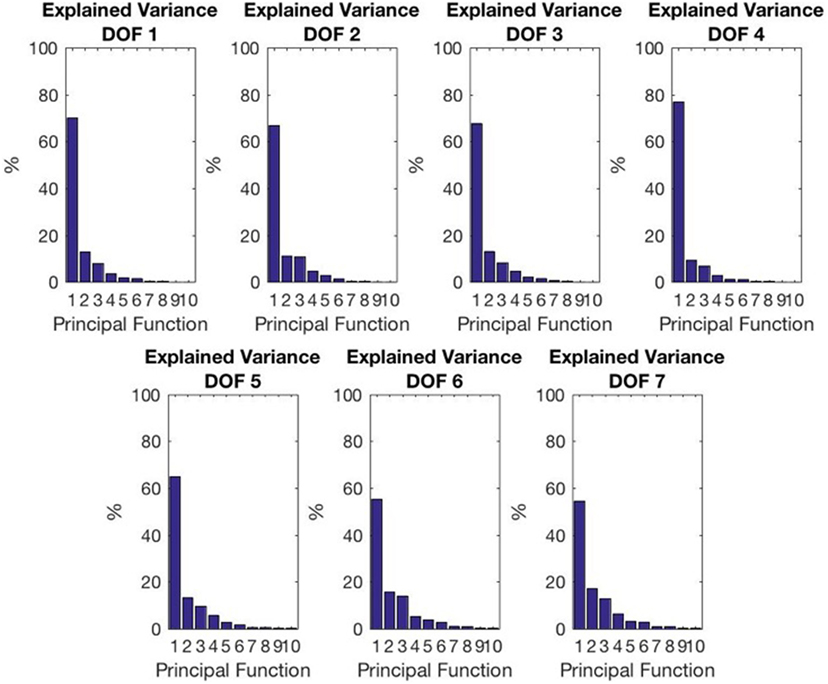
Figure 8. Explained variance for different DoFs and for each fPC.

FIGURE 9

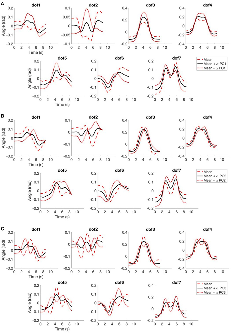
Figure 9. In (A), we report the mean function (in black) and the same mean function with the contribution of the first principal function, weighted with a coefficient α equal to one (with positive sign in red dashed line, with negative sign in red dotted line); in (B), we report the mean function (in black) and the same mean function with the contribution of the second principal function with a coefficient α equal to one (same legend of (A)); in (C), we report the mean function (in black) and the same mean function with the contribution of the third principal function with a coefficient α equal to one (same legend of (A)).

FIGURE 10

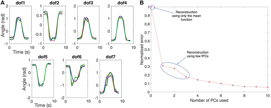
Figure 10. In (A) we show an example of trajectory reconstruction. The black line is the real data. The red line is the reconstructed data using the mean values and the first principal component. The blue line is the reconstructed data using the mean values and the first two principal components. The green line is the reconstructed data using the mean values and the first three principal components. In (B) we report the normalized reconstruction error (RMS). The initial point refers to the error when only the mean function is used for reconstruction. The other points refer to the error when one or more fPCs are used for the reconstruction.

Figure 10B reports a plot of the normalized error, calculated as E_RMS/max(E_RMS), for different number of fPCs used. Initial point refers to the case where only mean function is used for reconstruction and the value of E_RMS is 0.6 rad. The reconstruction using one fPC has an E_RMS value lower than 0.2 rad, adding other fPCs, the reconstruction error decay, i.e., using three fPCs the E_RMS value is around 0.1 rad. Furthermore, the whole reconstructed movement for the upper limb (considering all DoFs) was displayed using a visualization tool developed in MatLab, showing a high level of anthropomorphism and realism. We can conclude that the kinematic complexity of upper limb trajectories can be simplified and easily described using the mean function and few principal functional modes.

5. Conclusion and Implications for Robotics and Bioengineering

In this work, we have shown that the complexity of upper limb movements in activities of daily living can be described using a reduced number of functional principal components. To achieve this goal, we developed an experimental setup, which is based on kinematic recordings but also allows to include additional sensing modalities. Kinematic data are based on a 7 DoFs model and are quantified through a calibration-identification procedure. Collected data were used to characterize upper limb movements through functional analysis. The findings of this work can be used to pave the path toward a more accurate characterization of human upper limb principal modes, opening fascinating scenarios in rehabilitation, e.g., for automatic recognition of physiological and pathological movements (e.g., stroke affected subjects) through machine learning.

At the same time, the here reported results and future investigations could also offer a valuable inspiration for the design and control of robotic manipulators. First, recognizing that few principal modes describe most of kinematic variability could provide insights for a more effective planning and control of robotic manipulators. For the planning phase, using input trajectories as combinations of the main functional components, which explain most of the kinematic variability, could represent a successful initial guess to control the movement of the robot—eventually combined with a feedback correction. This combination of feedforward and feedback components could be successfully employed also with soft robotic manipulators, i.e., robots designed to embody safe and natural behaviors relying on compliant physical structures purposefully used to achieve desirable and sometimes variable impedance characteristics. In these cases, standard methods of robotic control can effectively fight against or even completely cancel the physical dynamics of the system, replacing them with a desired model—which defeats the purpose of introducing physical compliance. To overcome this limitation in Della Santina et al. (2017), an anticipative model of human motor control was proposed, which used a feedforward action combined with low-gain feedback, with the goal of obtaining human-like behavior through iterative learning. Results presented in this work could be used to define the feedforward component for the control of soft robots. Second, using human-like primitives for controlling robotic systems could improve the effectiveness and safety of human–robot interaction (HRI). Indeed, several studies identified anthropomorphism as one of the key enabling factor for successful, acceptable, predictable, and safe HRI in many fields, such as human robot co-working and rehabilitative/assistive robotics (Duffy, 2003; Bartneck et al., 2009; Riek et al., 2009; Dragan and Srinivasa, 2014). Furthermore, the here reported experimental and analytical framework could be used to identify principal actuation schemes for under-actuated robotic devices. As an example, in Casini et al. (2017), we used the identification procedure and the kinematic model reported in this work to estimate the contribution of wrist joints in the most common poses for grasping. We performed PCA on the estimated joints of the wrist pre-grasp poses and we found that the flexo-extension DoF plays a dominant role. We used these results to calibrate an under-actuated wrist system, which is also adaptable and allows to implement different under-actuation schemes, demonstrating its effectiveness to accomplish grasping and manipulation tasks. Future works will aim at using functional data to allow a dynamic implementation of principal kinematic modes of human upper limb in robotic systems. Finally, the integration of other sensing modalities, such as electro-encephalographic recordings, could be used to study neural correlates of human upper limb motions, thus possibly inspiring the development of effective brain–machine interfaces for assistive robotics.

Ethics Statement

This study was carried out in accordance with the recommendations of Regione Toscana, D.G.R. no. 158 23/02/2004, “Direttive regionali in materia di autorizzazione e procedure di valutazione degli studi osservazionali,” with written informed consent from all subjects in accordance with the Declaration of Helsinki, and in observation of the “Guideline for good clinical practice E6(R1), International Council for Harmonization of Technical Requirements for Pharmaceuticals for Human Use (ICH).” The protocol was approved by the local Ethical Committee, i.e., “Comitato Etico di Area Vasta Nord-Ovest (CEAVNO).”

Author Contributions

GA, CS, MB, and AB designed the study. GA, FF, and MB designed the protocol. GA, EB, and FF designed and developed the experimental setup. GA and FF performed the experiments. GA, CS, and MB performed data analysis. All authors contributed to writing the manuscript.

Conflict of Interest Statement

The authors declare that the research was conducted in the absence of any commercial or financial relationships that could be construed as a potential conflict of interest.

Funding

This work is supported by the European Commission H2020 grants “SOMA” (no. 645599) and SOFTPRO (no. 688857) and by the ERC Advanced Grant no. 291166 “SoftHands.”

References

Abdel-Malek, K., Yang, J., Brand, R., and Tanbour, E. (2004). Towards understanding the workspace of human limbs. Ergonomics 47, 1386–1405. doi: 10.1080/00140130410001724255

PubMed Abstract | CrossRef Full Text | Google Scholar

Aguilera, A. M., Ocaña, F. A., and Valderrama, M. J. (1999). Forecasting time series by functional PCA. Discussion of several weighted approaches. Comput. Stat. 14, 443–467. doi:10.1007/s001800050025

CrossRef Full Text | Google Scholar

Bartneck, C., Kulić, D., Croft, E., and Zoghbi, S. (2009). Measurement instruments for the anthropomorphism, animacy, likeability, perceived intelligence, and perceived safety of robots. Int. J. Soc. Robot. 1, 71–81. doi:10.1007/s12369-008-0001-3

CrossRef Full Text | Google Scholar

Benati, M., Gaglio, S., Morasso, P., Tagliasco, V., and Zaccaria, R. (1980). Anthropomorphic robotics. Biol. Cybern. 38, 125–140. doi:10.1007/BF00337403

CrossRef Full Text | Google Scholar

Berndt, D. J., and Clifford, J. (1994). “Using dynamic time warping to find patterns in time series,” in KDD Workshop, Vol. 10 (Seattle, WA), 359–370.

Google Scholar

Biryukova, E., Roby-Brami, A., Frolov, A., and Mokhtari, M. (2000). Kinematics of human arm reconstructed from spatial tracking system recordings. J. Biomech. 33, 985–995. doi:10.1016/S0021-9290(00)00040-3

PubMed Abstract | CrossRef Full Text | Google Scholar

Brockett, R. W. (1984). “Robotic manipulators and the product of exponentials formula,” in Mathematical Theory of Networks and Systems (Berlin, Heidelberg: Springer), 120–129.

Google Scholar

Butler, E. E., Ladd, A. L., Louie, S. A., LaMont, L. E., Wong, W., and Rose, J. (2010). Three-dimensional kinematics of the upper limb during a reach and grasp cycle for children. Gait Posture 32, 72–77. doi:10.1016/j.gaitpost.2010.03.011

PubMed Abstract | CrossRef Full Text | Google Scholar

Casini, S., Tincani, V., Averta, G., Poggiani, M., Della Santina, C., Battaglia, E., et al. (2017). “Design of an under-actuated wrist based on adaptive synergies,” in IEEE International Conference of Robotics and Automation, ICRA2017 (Singapore: IEEE).

Google Scholar

Coffey, N., Harrison, A. J., Donoghue, O., and Hayes, K. (2011). Common functional principal components analysis: a new approach to analyzing human movement data. Hum. Mov. Sci. 30, 1144–1166. doi:10.1016/j.humov.2010.11.005

PubMed Abstract | CrossRef Full Text | Google Scholar

Cubelli, R., Marchetti, C., Boscolo, G., and Della Sala, S. (2000). Cognition in action: testing a model of limb apraxia. Brain Cogn. 44, 144–165. doi:10.1006/brcg.2000.1226

PubMed Abstract | CrossRef Full Text | Google Scholar

Cutkosky, M. R. (1989). On grasp choice, grasp models, and the design of hands for manufacturing tasks. IEEE Trans. Robot. Autom. 5, 269–279. doi:10.1109/70.34763

CrossRef Full Text | Google Scholar

Dai, W., Sun, Y., and Qian, X. (2013). “Functional analysis of grasping motion,” in IEEE/RSJ International Conference on Intelligent Robots and Systems (Tokyo: IEEE), 3507–3513.

Google Scholar

d’Avella, A., and Lacquaniti, F. (2013). Control of reaching movements by muscle synergy combinations. Front. Comput. Neurosci. 7:42. doi:10.3389/fncom.2013.00042

PubMed Abstract | CrossRef Full Text | Google Scholar

d’Avella, A., Portone, A., Fernandez, L., and Lacquaniti, F. (2006). Control of fast-reaching movements by muscle synergy combinations. J. Neurosci. 26, 7791–7810. doi:10.1523/JNEUROSCI.0830-06.2006

PubMed Abstract | CrossRef Full Text | Google Scholar

d’Avella, A., and Tresch, M. C. (2002). Modularity in the motor system: decomposition of muscle patterns as combinations of time-varying synergies. Adv. Neural Inf. Process Syst. 1, 141–148.

Google Scholar

Della Santina, C., Bianchi, M., Grioli, G., Angelini, F., Catalano, M. G., Garabini, M., et al. (2017). Controlling soft robots: balancing feedback and feedforward elements. IEEE Robot. Autom. Mag. PP, 1–1. doi:10.1109/MRA.2016.2636360

CrossRef Full Text | Google Scholar

Dragan, A., and Srinivasa, S. (2014). Integrating human observer inferences into robot motion planning. Auton. Robots 37, 351–368. doi:10.1007/s10514-014-9408-x

CrossRef Full Text | Google Scholar

Duffy, B. R. (2003). Anthropomorphism and the social robot. Rob. Auton. Syst. 42, 177–190. doi:10.1016/S0921-8890(02)00374-3

CrossRef Full Text | Google Scholar

Feix, T., Romero, J., Schmiedmayer, H.-B., Dollar, A. M., and Kragic, D. (2016). The grasp taxonomy of human grasp types. IEEE Trans. Hum. Mach. Syst. 46, 66–77. doi:10.1109/THMS.2015.2470657

CrossRef Full Text | Google Scholar

Flash, T., and Hogan, N. (1985). The coordination of arm movements: an experimentally confirmed mathematical model. J. Neurosci. 5, 1688–1703.

PubMed Abstract | Google Scholar

Fu, K. C. D., Nakamura, Y., Yamamoto, T., and Ishiguro, H. (2013). Analysis of motor synergies utilization for optimal movement generation for a human-like robotic arm. Int. J. Autom. Comput. 10, 515–524. doi:10.1007/s11633-013-0749-2

CrossRef Full Text | Google Scholar

Gabiccini, M., Stillfried, G., Marino, H., and Bianchi, M. (2013). “A data-driven kinematic model of the human hand with soft-tissue artifact compensation mechanism for grasp synergy analysis,” in IEEE/RSJ International Conference on Intelligent Robots and Systems (Tokyo: IEEE), 3738–3745.

Google Scholar

Gokulakrishnan, P., Lawrence, A., McLellan, P., and Grandmaison, E. (2006). A functional-PCA approach for analyzing and reducing complex chemical mechanisms. Comput. Chem. Eng. 30, 1093–1101. doi:10.1016/j.compchemeng.2006.02.007

CrossRef Full Text | Google Scholar

Handjaras, G., Bernardi, G., Benuzzi, F., Nichelli, P. F., Pietrini, P., and Ricciardi, E. (2015). A topographical organization for action representation in the human brain. Hum. Brain Mapp. 36, 3832–3844. doi:10.1002/hbm.22881

PubMed Abstract | CrossRef Full Text | Google Scholar

Heidari, O., Roylance, J. O., Perez-Gracia, A., and Kendall, E. (2016). “Quantification of upper-body synergies: a case comparison for stroke and non-stroke victims,” in ASME 2016 International Design Engineering Technical Conferences and Computers and Information in Engineering Conference (Charlotte, NC: American Society of Mechanical Engineers), V05AT07A032.

Google Scholar

Holzbaur, K. R., Murray, W. M., and Delp, S. L. (2005). A model of the upper extremity for simulating musculoskeletal surgery and analyzing neuromuscular control. Ann. Biomed. Eng. 33, 829–840. doi:10.1007/s10439-005-3320-7

PubMed Abstract | CrossRef Full Text | Google Scholar

Lenarcic, J., and Umek, A. (1994). Simple model of human arm reachable workspace. IEEE Trans. Syst. Man Cybern. 24, 1239–1246. doi:10.1109/21.299704

CrossRef Full Text | Google Scholar

Lunardini, F., Casellato, C., d’Avella, A., Sanger, T., and Pedrocchi, A. (2015). Robustness and reliability of synergy-based myocontrol of a multiple degree of freedom robotic arm. IEEE Trans. Neural. Syst. Rehabil. Eng. 24, 940–950. doi:10.1109/TNSRE.2015.2483375

CrossRef Full Text | Google Scholar

Mason, C. R., Gomez, J. E., and Ebner, T. J. (2001). Hand synergies during reach-to-grasp. J. Neurophysiol. 86, 2896–2910.

PubMed Abstract | Google Scholar

Maurel, W., and Thalmann, D. (2000). Human shoulder modeling including scapulo-thoracic constraint and joint sinus cones. Comput. Graph. 24, 203–218. doi:10.1016/S0097-8493(99)00155-7

CrossRef Full Text | Google Scholar

Müller, M. (2007). “Chapter 4: Dynamic time warping,” in Information Retrieval for Music and Motion (Berlin, Heidelberg, New York: Springer Science+Business Media), 4, 69–84. doi:10.1007/978-3-540-74048-3_4

CrossRef Full Text | Google Scholar

Perry, J. C., Rosen, J., and Burns, S. (2007). Upper-limb powered exoskeleton design. IEEE/ASME Trans. Mechatron. 12, 408. doi:10.1109/TMECH.2007.901934

CrossRef Full Text | Google Scholar

Rabiner, L. R., Rosenberg, A. E., and Levinson, S. E. (1978). Considerations in dynamic time warping algorithms for discrete word recognition. J. Acoust. Soc. Am. 63, S79–S79. doi:10.1121/1.2016831

CrossRef Full Text | Google Scholar

Ramsay, J. O. (2006). Functional Data Analysis. Hoboken, NJ: Wiley Online Library.

Google Scholar

Ramsay, J. O., Hooker, G., and Graves, S. (2009). Functional Data Analysis with R and MATLAB. Berlin: Springer Science+Business Media.

Google Scholar

Ramsay, J. O., and Silverman, B. W. (2002). Applied Functional Data Analysis: Methods and Case Studies. New York: CiteSeer, 77.

Google Scholar

Riek, L. D., Rabinowitch, T.-C., Chakrabarti, B., and Robinson, P. (2009). “How anthropomorphism affects empathy toward robots,” in Proceedings of the 4th ACM/IEEE International Conference on Human Robot Interaction (La Jolla, CA: ACM), 245–246.

Google Scholar

Ryan, W., Harrison, A., and Hayes, K. (2006). Functional data analysis of knee joint kinematics in the vertical jump. Sports Biomech. 5, 121–138. doi:10.1080/14763141.2006.9628228

PubMed Abstract | CrossRef Full Text | Google Scholar

Salvador, S., and Chan, P. (2007). Toward accurate dynamic time warping in linear time and space. Intell. Data Anal. 11, 561–580.

Google Scholar

Santello, M. (2014). “Synergistic control of hand muscles through common neural input,” in The Human Hand as an Inspiration for Robot Hand Development (Cham: Springer), 23–48.

Google Scholar

Santello, M., Baud-Bovy, G., and Jörntell, H. (2013). Neural bases of hand synergies. Front. Comput. Neurosci. 7:23. doi:10.3389/fncom.2013.00023

PubMed Abstract | CrossRef Full Text | Google Scholar

Santello, M., Bianchi, M., Gabiccini, M., Ricciardi, E., Salvietti, G., Prattichizzo, D., et al. (2016). Hand synergies: integration of robotics and neuroscience for understanding the control of biological and artificial hands. Phys. Life Rev. 17, 1–23. doi:10.1016/j.plrev.2016.02.001

CrossRef Full Text | Google Scholar

Santello, M., Flanders, M., and Soechting, J. F. (1998). Postural hand synergies for tool use. J. Neurosci. 18, 10105–10115.

PubMed Abstract | Google Scholar

Schäling, B. (2011). The Boost C++ Libraries. Boris Schäling.

Google Scholar

Thakur, P. H., Bastian, A. J., and Hsiao, S. S. (2008). Multidigit movement synergies of the human hand in an unconstrained haptic exploration task. J. Neurosci. 28, 1271–1281. doi:10.1523/JNEUROSCI.4512-07.2008

PubMed Abstract | CrossRef Full Text | Google Scholar

Todorov, E., and Ghahramani, Z. (2004). “Analysis of the synergies underlying complex hand manipulation,” in Engineering in Medicine and Biology Society, 2004. IEMBS’04. 26th Annual International Conference of the IEEE, Vol. 2 (San Francisco, CA: IEEE), 4637–4640.

Google Scholar

Vinjamuri, R., Sun, M., Chang, C.-C., Lee, H.-N., Sclabassi, R. J., and Mao, Z.-H. (2010). Temporal postural synergies of the hand in rapid grasping tasks. IEEE Trans. Inf. Technol. Biomed. 14, 986–994. doi:10.1109/TITB.2009.2038907

PubMed Abstract | CrossRef Full Text | Google Scholar

Zatsiorsky, V. M., and Latash, M. L. (2004). Prehension synergies. Exerc. Sport Sci. Rev. 32, 75. doi:10.1097/00003677-200404000-00007

PubMed Abstract | CrossRef Full Text | Google Scholar