Non-Parametric Bayesian State Space Estimator for Negative Information

1. Introduction

Estimating the location of a mobile agent while simultaneously building a map of the environment has been regarded as one of the most important problems to be solved for agents to achieve autonomy. It is a necessary precondition for any agent to have an estimation of the world to store acquired knowledge. There has been a vast amount of research surrounding the field of Simultaneous Localization And Mapping (SLAM) that branches out into a wide variety of subfields dealing with problems from building accurate noise models of the agent sensors (Plagemann et al., 2007), to determining which environmental feature caused a particular measurement, also known as the data association problem (Montemerlo and Thrun, 2003) and much more.

Although the amount of research might seem overwhelming at first, all current SLAM methodologies are founded on a single principle: As the agent localizes itself by reducing its position uncertainty, the map’s uncertainty also decreases as the landmarks are correlated via the robot’s position (Durrant-Whyte and Bailey, 2006). The predominant mathematical formulation of SLAM problems is to parameterize the joint distribution of the agent’s position and map’s features and to recursively integrate actions and measurement information into those parameters. This formulation is known as Probabilistic-SLAM (Durrant-Whyte and Bailey, 2006; Cadena et al., 2016) and there are broadly three paradigms to parameterizing.

The first paradigms assume the joint distribution to be a Multivariate Gaussian distribution parameterized by a mean and covariance. The mean is a state vector composed of the agent and map feature positions while the elements of the covariance encode the variance of the position uncertainties. If the motion and measurement system models are linear the Kalman Filter recursion is the best estimator of the joint’s parameters. In case, the system models are non-linear they can be linearized via a Taylor approximation and in the context of SLAM, this is known as EKF-SLAM (Extended-Kalman Filter) (Durrant-Whyte and Bailey, 2006). The two drawbacks of EKF-SLAM are the linearization of the system models, which may falsely reduce uncertainty resulting in the filter diverging (Li and Mourikis, 2013), and the quadratic growth of the filter’s parameters with respect to the number of landmarks (Paz et al., 2008). The linearization problem has been addressed by non-parametric approaches, such as Unscented Kalman Filter (Wan and Van Der Merwe, 2000; Huang et al., 2013), which avoid the linearization by using a set of deterministic samples, known as sigma points or by introducing constraints on the Jacobian of the system models (Mourikis and Roumeliotis, 2007). The constraint approach has been shown to be robust and scalable. In Hesch et al. (2014), the authors introduce a constraint on the Jacobians of both motion and measurement system models, which explicitly enforces that no unwanted information is gained. The authors successively mapped 1.5 km of the outdoor terrain at the Minnesota campus. In terms of the quadratic growth drawback parameter, efficient EKF methods have been developed known as Extended information Filters (Thrun et al., 2004). The methods use a canonical parameterization of the Gaussian function that includes the precision matrix, which is sparse. The drawback of information filters is that extracting the variance of the position uncertainty requires inverting the precision matrix, which is computationally expensive. Since then there are methods that decompose the EKF-SLAM problem and are able to solve it in linear time (Paz et al., 2008). Although EKF-SLAM originally suffered from linearization and computational cost the scientific advances mentioned above still make it a method of choice (Cadena et al., 2016). Especially when the linearization of the system models are accurate as it is the case with vision-SLAM methods such as visual-inertial odometry VIO-SLAM (Li and Mourikis, 2013). EKF-SLAM methods also remain widely used in underwater navigation problems, the reader is referred to Paull et al. (2014) and Hidalgo and Brunl (2015) for a review.

The second paradigm is Graph-SLAM (Grisetti et al., 2010). Graph-SLAM methods find the Maximum A Posteriori (MAP) of the full robot path in contrast to EKF-SLAM methods that are filters. As the name suggests a directed graph is gradually constructed with nodes being robot positions and edges geometric transformation between them. The transformations are non-linear constraints, which are measurement likelihoods with an error assumed to be Gaussian noise. The MAP solution of the robot’s path is equivalent to solving a non-linear least square problem whose solution is attained by a Gauss–Newton optimization (Kuemmerle et al., 2011). This process results in the repositioning of the nodes such that the measurement constraints are minimized. Graph-based approaches are becoming increasingly popular as MAP solutions are more robust when compared to filtering approaches (Cadena et al., 2016). As a result, multiple Graph-SLAM solvers have been released such as Large Scale-Directed monocular SLAM (LSD-SLAM) (Engel et al., 2014), which can handle environments with different scales and is able to build large indoor and outdoor density maps, and ORB-SLAM (Mur-Artal et al., 2015; Mur-Artal and Tardos, 2016), which uses ORB (Rublee et al., 2011) features extracted from keyframes. Recent developments in the context of vision-SLAM efforts have focused on efficiency and extraction of the pose uncertainty (Ila et al., 2017) as Graph-SLAM methods generally only find the mean trajectory of the robot and not its variance. Graph-SLAM approaches mostly differ in the type of feature extraction methods (known as the front-end) while retain the same non-linear solver (bundle adjustment) such as g2o (Kuemmerle et al., 2011).

The third paradigm is FastSLAM (Montemerlo et al., 2003). FastSLAM exploits the fact that if we know the agent’s position with certainty all landmarks become independent. It models the distribution of the agent’s position by a particle filter. Each particle has its own copy of the map and updates all landmarks independently, which is the strength of this method. However, if many particles are required each must have its own copy of the map. FastSLAM methods have less traction in the literature as difficulties include tuning the resampling strategy, which if not dune properly can result in sample impoverishment.

It is beyond the scope of this chapter to provide a detailed review of these three paradigms. The reader is referred to Thrun et al. (2005), Thrun and Leonard (2008) for an introductory material.

1.1. Problem Statement

We consider an agent searching for a set of objects in a partially known environment in which exteroceptive feedback is extremely limited. For instance, we can think of an agent equipped with a range sensor that returns a positive response when in direct contact with an object and no response otherwise. Consider agent living in a Rectangle world, see Figure 1, in which is located two objects. The agent’s uncertainty of its location and that of the objects is encoded by probability distributions P(⋅), which at initialization are known as the agent’s prior beliefs.

FIGURE 1

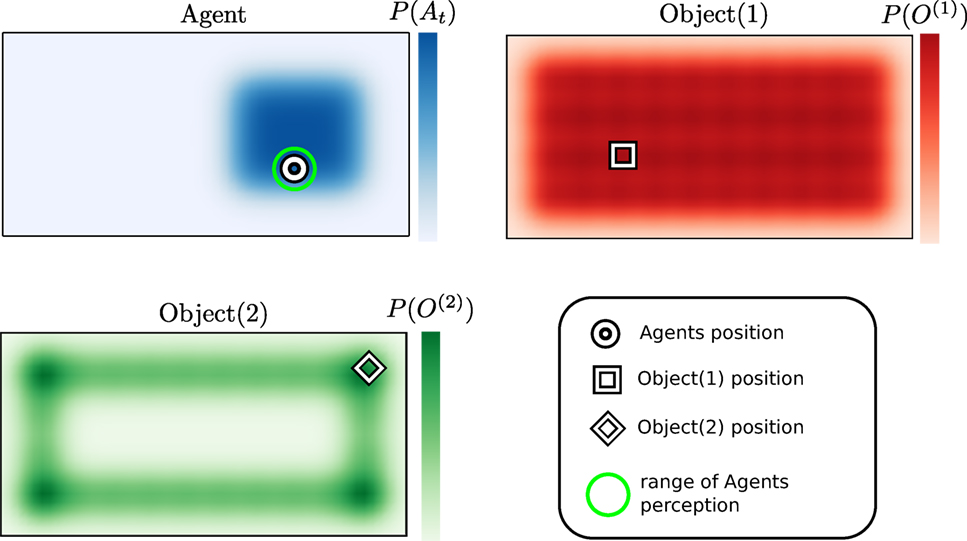
Figure 1. Rectangle world. There are three different probability density functions present. The blue represents the believed location of the agent, the red and green probability distributions are associated with objects 1 and 2. The white shapes in each figure represent the true location of each associated object or agent.

As the agent explores the world, it integrates all sensing information at each time step and updates its prior beliefs to posteriors (the result of the prior belief after integrating motion and sensory information). To the author’s knowledge, current SLAM methods are limited in that they consider only uncertainty induced by sensing inaccuracies inherent in the sensor and motion models. The reason for this widespread limitation is that during the theoretical foundation of SLAM, a period that is referred to as the classic age (1986–2004) (Cadena et al., 2016) (this period gave the three paradigms discussed above), the application domains considered the signal noise in range sensor, cameras, and odometry measurements. The features were always considered to be measurable except when occluded. In our setting as the sensory information is strictly haptic, we can confidently assume no measurement noise.

In the search task illustrated in Figure 1, the prior beliefs and sparse measurements are the two sources of the agent’s uncertainty. The absence of a positive measurement (detection of an object of instance) is known as negative information (Thrun, 2002; Hoffman et al., 2005; Thrun et al., 2005, p. 313). Thus, SLAM methodologies that use the Gaussian error between the predicted and estimated position of features, such as in the case of EKF-SLAM and Graph-SLAM, will not perform well in this setting as no measurements of the features positions are available until our agent “bumps” into a feature.

In addition to the negative sensing information, the original beliefs depicted in Figure 1 are non-Gaussian and multimodal. We make no assumption regarding the form of the beliefs. This implies that the joint distribution can no longer be parameterized by a Multivariate Gaussian. This is an assumption made in many SLAM algorithms, notably EKF-SLAM, and allows for a closed form solution to the state estimation problem. Without the Gaussian assumption, no closed form solution to the filtering problem is feasible. Using standard non-parametric methods (Kernel Density, Gaussian Process, Histogram, etc.) to represent or estimate the joint distribution becomes unrealistic after a few dimensions or additional map features. FastSLAM could be a potential candidate, however, as it parameterizes the position uncertainty of the agent by a particle filter and each particle has its own copy of the map the memory demands become quickly significant and in addition has been shown that FastSLAM can degenerate with time regardless of the number of particles used (Bailey et al., 2006). For planning purposes, we would also want to have a single representation of the marginals. The box below summarizes the desirable attributes and assumptions for our filter.

---

Attributes and Assumptions

• Non-Gaussian joint distribution, no assumptions are made with respect to its form.

• Mostly negative information available (absence of positive sightings of the landmarks).

• Joint distribution volume grows exponentially with respect to the number of objects and states.

• Joint distribution volume is dense, there is high uncertainty.

---

1.2. The Contribution to the Field of Artificial Intelligence

In a wide range of Artificial Intelligence (AI) applications the agent’s beliefs are discrete. This non-parametric representation is the most unconstraining but comes at a cost. The parameterization of the belief’s joint distribution grows at the rate of a double exponential. We propose a Bayesian State Space Estimator (BSSE) which delivers the same filtered beliefs as a traditional filter but without explicitly parametrizing the joint distribution. We refer to our novel filter as the Measurement Likelihood Memory Filter (MLMF). It keeps track of the history of measurement likelihood functions, referred to as the memory, which have been applied to the joint distribution. The MLMF filter efficiently processes negative information. To the author’s knowledge, there has been little research on the integration of negative information in an SLAM setting. Previous work considered the case of active localization (Hoffmann et al., 2006). The incorporation of negative information is useful in many contexts and in particular in Bayesian Theory of Mind (Bake et al., 2011), where the reasoning process of a human is inferred from a Bayesian Network and in our own work (de Chambrier and Billard, 2013) where we model the search behavior of an intentionally blinded human. In such a setting, much negative information is present and an efficient belief filter is required. Our MLMF is thus applicable to the SLAM and AI community in general and to the Cognitive Science community, which models human or agent behaviors through the usage of Bayesian state estimators.

By using this new representation, we implement a set of passive search trajectories through the state space and demonstrate, for a discretized state space, that our novel filter is optimal with respect to the Bayesian criteria (the successive filtered posteriors are exact and not an approximation with respect to Bayes rule). We provide an analysis of the space and time complexity of our algorithm and prove that it is always more efficient even when considering worst-case scenarios. Finally, we consider an Active-SLAM setting and evaluate how constraining the size of the number of memorized likelihood functions impact the decision-making process of a greedy one-step look-ahead planner.

The rest of the document is structured as follows: in section 2, we overview the Bayes filter recursion and apply it to a simple 1D search scenario for both a discrete and Gaussian parametrization of the beliefs. We demonstrate that discrete parametrization gives the correct filtered beliefs but at a very high cost and that the EKF-SLAM fails to provide the adequate solution. In section 3, we introduce the Measurement Likelihood Memory Filter and overview its parametrization. In section 4, we derive the computational time and space complexity of the MLMF. Section 5 describes additional assumptions made with respect to the MLMF to make it scalable (scalable-MLMF). In section 6, we numerically evaluate the time complexity of the scalable-MLMF and check the assumption we made for it to be scalable. We investigate the filter’s sensitivity with respect to its parameters in an Active-SLAM setting.

2. Bayesian State Space Estimation with Negative Information

Bayesian State Space Estimators (BSSE) recursively incorporate actions u_t and observations y_t into a prior joint distribution P(A_t, O|Y_0:t−1, u_1:t−1) to obtain a posterior joint distribution P(A_t, O|Y_0:t, u_1:t) through the application of Bayes rules. The agent’s random variable, A, is associated with the uncertainty of its location in the world, the same holds for the object(s’) random variable(s), O. This is also known as the SLAM filtering problem. In Figure 2, we depict the general Bayesian Network (BN) of a BSSE, which conveys the dependence and independence relation between the random variables. The conditional dependence $A╥O|Y$ is necessary for incorporating information into the joint distribution and decreasing the uncertainty. The strength of the conditional dependence is governed by the size of the change the measurement likelihood P(Y_t|A_t, O) function has on the joint distribution. If the measurement likelihood does not affect the joint distribution, then the agent and object random variables will be independent, A ╨ O. If they are independent, then no information acquired by the agent can be used to infer changes in the object estimates.

FIGURE 2

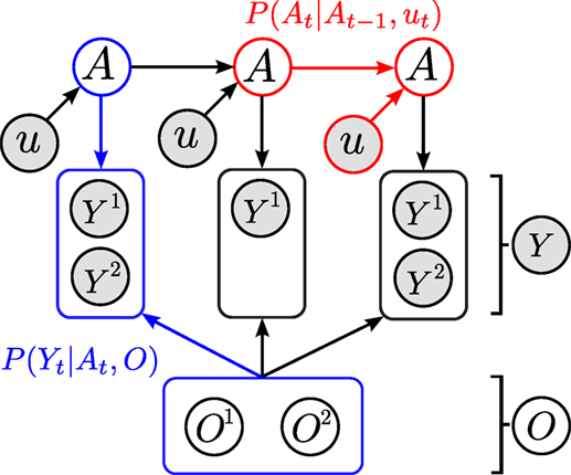
Figure 2. Directed graphical model of dependencies between the agent (A) and object (O)’s estimated location. Each object, O⁽ⁱ⁾ is associated with one sensing random variable Y⁽ⁱ⁾. The overall sensing random variable is Y = [Y⁽¹⁾,…,Y^(M−1)]^T, where M is the total number of agent and object random variables in the filter. For readability, we have left out the time index t from A and Y. Since the objects are static, they have no temporal process associated with them thus they will never have a time subscript. The two models necessary for filtering are the motion model P(A_t|A_t−1, u_t) (red) and measurement model P(Y_t|A_t, O) (blue).

We next demonstrate the effect negative information has on the update of the joint distribution for two different parameterizations, namely, for EKF and Histogram.

2.1. EKF-SLAM

In EKF-SLAM, the joint density p(A_t, O|Y_0:t, u_1:t; μ_t, Σ_t) is a multivariate Gaussian function parametrized by a mean μ_t and covariance Σ_t. For simplicity, we considering a 1D search of one object. In this setting, the mean of the agent ${\mu }_{a_t}\in \mathbb{R}$ and object are μ_o ∈ ℝ are 1D Cartesian positions

${\mathit{\mu }}_t={[{\mu }_{a_t},{\mu }_o]}^{\text{T}}\in {ℝ}^{(2\times 1)}{\mathrm{\Sigma }}_t=\left[\begin{array}{cc}{\mathrm{\Sigma }}_a& {\mathrm{\Sigma }}_{ao}\\ {\mathrm{\Sigma }}_{oa}& {\mathrm{\Sigma }}_o\end{array}\right]\in {ℝ}^{(2\times 2)}.$ (1)

The measurement Y_t ∈ [0, 1] of the object by the agent is simulated by a radial basis function as is the measurement function (equation (2))

${\widehat{Y}}_t=\exp \left(-\frac{1}{2{\sigma }^2}||A_t-O{||}^2\right).$ (2)

By setting the variance σ² to be small, we can approximate a smooth binary sensor. EKF-SLAM assumes that the measurement is corrupted by Gaussian noise, ϵ ∼𝒩(0, R), giving the likelihood function:

$p\left(Y_t\mathrm{|}{A}_t,O_t\right)=\frac{1}{\mathrm{|}\text{2}\pi R{\mathrm{|}}^{\frac{1}{2}}}\exp \left(-\frac{1}{2}\left(\right.Y_t-{\widehat{Y}}_t{\left)\right.}^{\mathrm{T}}{R}^{-1}\left(\right.Y_t-{\widehat{Y}}_t\left)\right.\right)$ (3)

where the covariance, R, encompasses the uncertainty in the measurement. The elements of the covariance matrix capture the measurement error between the true Y and expected measurement $\widehat{Y}$. As the joint distribution is parameterized by a single Multivariate Gaussian, a closed form solution to the filtering equations exists, called the Kalman Filter (Durrant-Whyte and Bailey, 2006).

In the search task, the agent can only perceive the object when in direct contact. This results in the observation Y_t being mostly always equal to $\widehat{Y}$. As a result, the agent’s uncertainty of his location and of the object only changes once the object is found, which is unhelpful during a search. This is because the magnitude of the error between the true and expected measurement $e=\left(Y_t-{\widehat{Y}}_t\right)$ directly affects the joint distribution and is zero during most of the search. Figure 3 illustrates this for the 1D search. The multivariate Gaussian parameterization of the joint and likelihood function only guarantees a dependency between the agent and object random variables when there is a positive sighting of the landmarks. This can be seen in Figure 3B, where the component Σ_ao is 0 most of the time implying A_t ╨ O|Y, which is undesirable. The EKF parameterization in this form is ill suited for search tasks in which negative information is predominant.

FIGURE 3

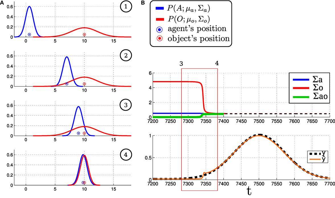
Figure 3. (A) EKF-SLAM time slice evolutions of the agent and object location belief for a 1D search. The temporal ordering is given by the numbers in the top right corner of each plot. The blue pdf represents the agent’s believed location, and the circle is the agent’s true location. The same holds for the red distribution that represents the agent’s belief of the location of an object. (B) Evolution of the covariance components of Σ over time and true Y_t and expected measurements, ${\widehat{Y}}_t$. Σ_a and Σ_o are the variances of the agent and object positions, and Σ_ao is the cross-covariance term.

2.2. Histogram-SLAM

In histogram-SLAM, the joint distribution is discretized, and each bin has a parameter, P(A_t = i, O = j|Y_0:t, u_1:t; θ) = θ^(ij) and all sum to one Σ_ijθ^(ij) = 1. For shorthand notation, we will write P(A_t, O|Y_0:t, u_1:t) instead of P(A_t = i, O = j|Y_0:t, u_1:t; θ). The probability distribution of the agent’s position is given by marginalizing the object random variable:

$P(A_t\mathrm{|}{Y}_{0:t,}{u}_{1:t;}{\mathit{\theta }}_a)={\displaystyle \sum _{j=1}^{\mathrm{|}o\mathrm{|}}P(A_{t,}O=j\mathrm{|}{Y}_{0:t,}{u}_{1:t;}\mathit{\theta }}).$ (4)

The converse holds true for the object’s marginal, that is the summation would be over the agent’s variable. We consider a similar 1D search task as the one used for EKF-SLAM. The world of the agent and object is discretized to 10 states, producing a joint distribution with 100 parameters, see Figure 4 (Top) for an illustration of the joint distribution. An observation occurs, as before, only if the agent enters in contact with the object, making the measurement and expected measurement binary Y_t ∈ {0, 1}. Equation (5) is the form of the likelihood function when the object is sensed by the agent

$P\left(Y_t=\mathbf{\text{1}}|A_t,O\right)=\left\{\begin{array}{cc}1\hfill & \text{if\hspace{0.17em}}{A}_t=O\hfill \\ 0\hfill & \text{if\hspace{0.17em}}{A}_t\ne O.\hfill \end{array}\right.$ (5)

FIGURE 4

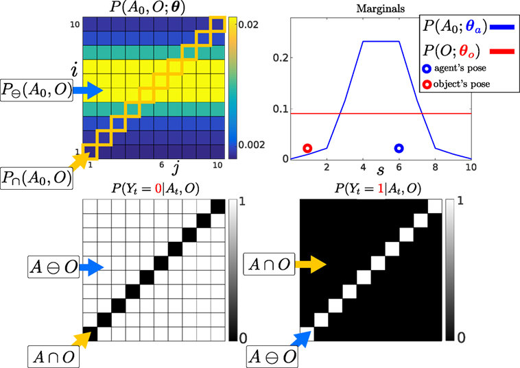
Figure 4. Top: Left: Initialization of the agent and object joint distribution. Right: Marginals of the agent and object parameterized by θ_a and θ_o, giving the probability of their location. The marginal of each random variable is obtained from equation (4). The probability of the agent and object being in state s = 6 is given by summing the blue and red highlighted parameters in the joint distribution. Bottom: 1D world Likelihood P(Y_t|A_t, O), the white regions A ∩ O will leave the joint distribution unchanged while the black regions will evaluate the joint distribution to zero. Left: No contact detected with the object, the current measurement is Y_t = 0, both the agent and object cannot be in the same state. Right: The agent entered into contact with the object and received a haptic feedback Y_t = 1. The agent receives only two measurement possibilities, contact or no contact.

Figure 4 (Bottom left) illustrates the likelihood function in the case of no contact Y_t = 0. When there is no contact with the object all the parameters of the joint distribution in the black regions become zero, which we refer to as the dependent states A ∩ O of the joint distribution. The white states are the independent states A⊖O, they are not changed by the likelihood function. The values of the joint distribution in the independent states will be unchanged by the likelihood function: P_⊖(A_t, O|Y_0:t, u_1:t) ∝ P_⊖(A_t, O|Y_0:t−1, u_1:t).

When the object is detected (Bottom right) the likelihood constrains all non-zero values of the joint distribution to be in states i = j, which in the case of a 2-dimensional joint distribution is a line. The sparsity of the likelihood function will be key to the development of the MLMF filter.

---

Histogram Bayesian recursion

Intialization

$P(A_0,O;\mathit{\theta })=P(A_0;{\mathit{\theta }}_a)P(O;{\mathit{\theta }}_o)={\mathit{\theta }}_a\times {\mathit{\theta }}_o$ (6)

Motion

$\mathit{\text{P}}\left({\mathit{\text{A}}}_{\mathit{\text{t}}},\mathit{\text{O}}|{\mathit{\text{Y}}}_{\mathrm{0:}\mathit{t}-\text{1}},{\mathit{\text{u}}}_{\text{1:}t}\right)={\displaystyle \sum _{A_{t-1}}}\mathit{\text{P}}\left({\mathit{\text{A}}}_{\mathit{\text{t}}}|{\mathit{\text{A}}}_{\mathit{\text{t}}-\text{1}},{\mathit{\text{u}}}_{\mathit{\text{t}}}\right)P\left({\mathit{\text{A}}}_{\mathit{\text{t}}-\text{1}},{\mathit{\text{O}}}_{\mathit{\text{t}}}|{\mathit{\text{Y}}}_{\mathrm{0:}t-\text{1}},{\mathit{\text{u}}}_{\text{1:}t-\text{1}}\right)$ (7)

Measurement

$\mathit{\text{P}}\left({\mathit{\text{A}}}_{\mathit{\text{t}}},\mathit{\text{O}}|{\mathit{\text{Y}}}_{\mathrm{0:}t},{\mathit{\text{u}}}_{\text{1:}t}\right)=\frac{\mathit{\text{P}}\left({\mathit{\text{Y}}}_{\mathit{\text{t}}}|{\mathit{\text{A}}}_{\mathit{\text{t}}},\mathit{\text{O}}\right)P\left({\mathit{\text{A}}}_{\mathit{\text{t}}},\mathit{\text{O}}|{\mathit{\text{Y}}}_{\mathrm{0:}t-\text{1}},{\mathit{\text{u}}}_{\text{1:}t}\right)}{\mathit{\text{P}}\left({\mathit{\text{Y}}}_{\mathit{\text{t}}}|{\mathit{\text{Y}}}_{\mathrm{0:}t-\text{1}},{\mathit{\text{u}}}_{\text{1:}t}\right)}$ (8)

---

Figure 5 illustrates the evolution of the joint distribution in a 1D example by applying the filtering Bayesian recursion equations (7) and (8). The agent and object’s true positions (unobservable) are in state 6 and 1. The agent moves three steps toward state 10. At each time step, as the agent fails to sense the object, the likelihood function P(Y_t = 0|A_t, O) (Figure 4, Bottom left) is applied. As the agent moves toward the right, the motion model shifts the joint distribution toward state 10 along the agent’s dimension, i (note that state 1 and 10 are wrapped). As the agent moves to the right more, joint distribution parameters become zero. The re-normalization by the evidence (denominator of equation (8)), which increases the value of the remaining parameters, is equal to the sum of the probability mass, which was set to zero by the likelihood function. Thus, the values of the parameters of the joint distribution that fall on the pink line in Figure 5 (green line also, but only for first time slice) become zero, and their values are redistributed to the remaining non-zero parameters.

FIGURE 5

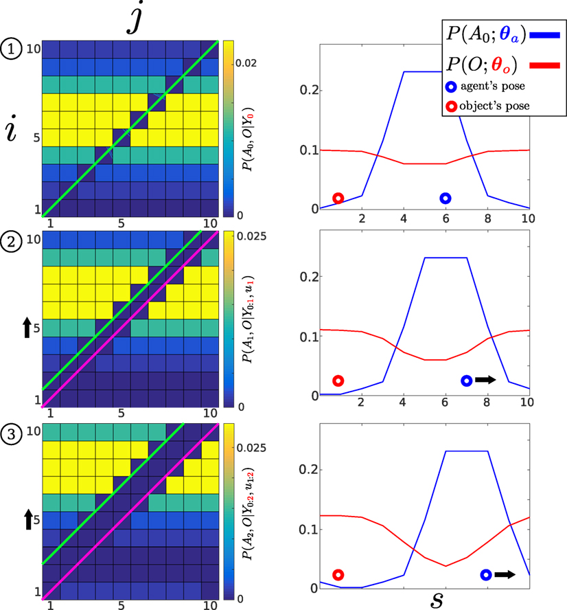
Figure 5. Histogram-SLAM, 4 time steps. (1) Application of likelihood P(Y₀ = 0|A₀, O) and the agent remains stationary, all states along the green line become zero. (2) The agent moves to the right u₁ = 1, the motion P(A₁|A₀, u₁), and likelihood models are applied consecutively. The right motion results in a shift (black arrow on the left) in the joint probability distribution toward the state i = 10. All parameters on the pink line are zero. (3) Same as two. At each time step, a new likelihood function (pink line) is applied to the joint distribution.

The inconvenience with histogram-SLAM is that its time and space complexity is exponential as the joint distribution is discretized and parametrized by θ^(ij). Instead, we propose a new filter, MLMF, which we formally introduce in the next section. This filter achieves the same result as the Histogram filter but without having to parameterize the values of the joint distribution, thus avoiding the exponential growth cost.

3. Measurement Likelihood Memory Filter

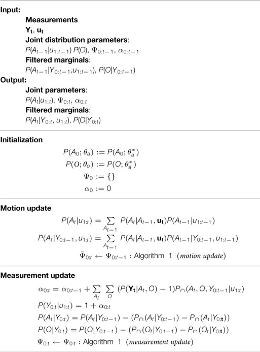
MLMF keeps a function parameterization of the joint distribution instead of a value parameterization as it is the case for histogram-SLAM. At initialization the joint distribution is represented by the product of marginals, equation (9), which would result in the joint distribution illustrated in Figure 4, if it were to be evaluated at all states (i, j) as it is done for histogram-SLAM. MLMF will only evaluate this product, when necessary, at specific states. At each time step, the motion and measurement update are applied (equations (10) and (11)). An important distinction is that these updates are performed on the un-normalized joint distribution P(A_t, O, Y_0:t|u_1:t), which is not the case in histogram-SLAM where the updates are done on the conditional P(A_t, O|Y_0:tu_1:t). After applying multiple motion and measurement updates the resulting joint distribution is given by equation (12), see Appendix C for a step-by-step derivation.

---

MLMF Bayesian filter

Joint marginals (initial)

$P(A_0,O)=P(A_0;\mathit{\theta }{}_a^{*})P(O;\mathit{\theta }{}_o^{*})$ (9)

Motion

$\mathit{\text{P}}\left({\mathit{\text{A}}}_{\mathit{\text{t}}},\mathit{\text{O}},{\mathit{\text{Y}}}_{\mathrm{0:}t-\text{1}}|{\mathit{\text{u}}}_{\text{1:}t}\right)={\displaystyle \sum _{A_{t-1}}}\mathit{\text{P}}\left({\mathit{\text{A}}}_{\mathit{\text{t}}}|{\mathit{\text{A}}}_{\mathit{\text{t}}-\text{1}},{\mathit{\text{u}}}_{\mathit{\text{t}}}\right)P\left({\mathit{\text{A}}}_{\mathit{\text{t}}-\text{1}},\mathit{\text{O}},{\mathit{\text{Y}}}_{\mathrm{0:}t-\text{1}}|{\mathit{\text{u}}}_{\text{1:}t-\text{1}}\right)$ (10)

Measurement

$\begin{array}{llll}\hfill & \mathit{\text{P}}\left({\mathit{\text{A}}}_{\mathit{\text{t}}},\mathit{\text{O}},{\mathit{\text{Y}}}_{\mathrm{0:}t}|{\mathit{\text{u}}}_{\text{1:}t};\mathit{\theta }{}_{\mathit{\text{o}}}^{\ast },\mathit{\theta }{}_{\mathit{\text{a}}}^{\ast },{\mathbf{\Psi }}_{\text{0:}\mathit{t}}\right)=& \hfill & \\ \hfill & \mathit{\text{P}}\left({\mathit{\text{Y}}}_{\mathit{\text{t}}}|{\mathit{\text{A}}}_{\mathit{\text{t}}},\mathit{\text{O}}\right)P\left(\mathit{\text{O}};\mathit{\theta }{}_{\mathit{\text{o}}}^{\ast }\right)P\left({\mathit{\text{A}}}_{\mathit{\text{t}}}|{\mathit{\text{u}}}_{\text{1:}t};\mathit{\theta }{}_{\mathit{\text{a}}}^{\ast }\right)P\left({\mathit{\text{Y}}}_{\mathrm{0:}t}|{\mathit{\text{A}}}_{\mathit{\text{t}}},\mathit{\text{O}},{\mathit{\text{u}}}_{\text{1:}t};{\overline{\mathbf{\Psi }}}_{\text{0:}t}\right)\end{array}$ (11)

Joint

$\mathit{\text{P}}\left({\mathit{\text{A}}}_{\mathit{\text{t}}},\mathit{\text{O}}|{\mathit{\text{Y}}}_{\mathrm{0:}t},{\mathit{\text{u}}}_{\text{1:}t};\mathit{\theta }{}_{\mathit{\text{o}}}^{\ast },\mathit{\theta }{}_{\mathit{\text{a}}}^{\ast },{\mathbf{\Psi }}_{\text{0:t}},\mathit{\alpha }{}_{\mathbf{\text{0:t}}}\right)=\frac{\mathit{\text{P}}\left({\mathit{\text{A}}}_{\mathit{\text{t}}},\mathit{\text{O}},{\mathit{\text{Y}}}_{\mathrm{0:}t}|{\mathit{\text{u}}}_{\text{1:}t};\mathit{\theta }{}_{\mathit{\text{o}}}^{\ast },\mathit{\theta }{}_{\mathit{\text{a}}}^{\ast },{\mathbf{\Psi }}_{\mathrm{0:}t}\right)}{\mathit{\text{P}}\left({\mathit{\text{Y}}}_{\mathrm{0:}t}|{\mathit{\text{u}}}_{\text{1:}t};\mathit{\alpha }{}_{\mathbf{\text{0:t}}}\right)}$ (12)

Filtered marginal

$\begin{array}{ll}\hfill & \mathit{\text{P}}\left({\mathit{\text{A}}}_{\mathit{\text{t}}}|{\mathit{\text{Y}}}_{\mathrm{0:}\mathbf{\text{t}}};{\mathit{\theta }}_{\mathit{\text{a}}}\right)=\mathit{\text{P}}\left({\mathit{\text{A}}}_{\mathit{\text{t}}}|{\mathit{\text{Y}}}_{\mathrm{0:}\mathbf{\text{t-1}}};{\mathit{\theta }}_{\mathit{\text{a}}}\right)-\left({\mathit{\text{P}}}_{\cap }\left({\mathit{\text{A}}}_{\mathit{\text{t}}}|{\mathit{\text{Y}}}_{\mathrm{0:}t-\text{1}}\right)-{\mathit{\text{P}}}_{\cap }\left({\mathit{\text{A}}}_{\mathit{\text{t}}}|{\mathit{\text{Y}}}_{\mathrm{0:}t}\right)\right)\end{array}$ (13)

$\begin{array}{ll}\hfill & \mathit{\text{P}}\left(\mathit{\text{O}}|{\mathit{\text{Y}}}_{\mathrm{0:}\mathbf{\text{t}}};{\mathit{\theta }}_{\mathit{\text{o}}}\right)=\mathit{\text{P}}\left(\mathit{\text{O}}|{\mathit{\text{Y}}}_{\mathrm{0:}\mathbf{\text{t-1}}};{\mathit{\theta }}_{\mathit{\text{o}}}\right)-\left({\mathit{\text{P}}}_{\cap }\left({\mathit{\text{A}}}_{\mathit{\text{t}}}|{\mathit{\text{Y}}}_{\mathrm{0:}t-\text{1}}\right)-{\mathit{\text{P}}}_{\cap }\left({\mathit{\text{A}}}_{\mathit{\text{t}}}|{\mathit{\text{Y}}}_{\mathrm{0:}t}\right)\right)\end{array}$ (14)

---

The MLFM filter is parameterized by the agent and object joint marginals $P\left(A_t\mathrm{|}{u}_{1_{:}t};\mathrm{\theta }{}_a^{\ast }\right)$, $P\left(O;\mathrm{\theta }{}_o^{\ast }\right)$, the filtered marginals $P\left(A_t\mathrm{|}{Y}_{0:t},u_{1:t};{\mathit{\theta }}_a\right)$ (u_1:t not shown in the above box), $P\left(O\mathrm{|}{Y}_{0:\mathbf{\text{t}}};{\mathrm{\theta }}_o\right)$, the evidence $P\left(Y_{0:t}\mathrm{|}{u}_{1:t};{\mathrm{\alpha }}_{\mathbf{\text{0}}:\mathbf{\text{t}}}\right)$ and the history of likelihood functions, $P\left(Y_{0:t}\mathrm{|}{A}_t,O,u_{1:t};{\mathrm{\Psi }}_{\mathbf{0:}\mathit{\text{t}}}\right)$, equation (15), which is the product of all the likelihood functions since initialization and we will refer to it as the memory likelihood function:

$P\left(Y_{0:t}\mathrm{|}{A}_t,O,u_{1:t};{\mathrm{\Psi }}_{\mathbf{0:}\mathit{\text{t}}}\right):={\displaystyle \prod _{i=0}^t}P\left(Y_i\mathrm{|}{A}_t,O,u_{i+1:t};l_i\right)$ (15)

$P\left(Y_i=\mathrm{0|}{A}_t,O,u_{i+1:t};l_i\right):=\left\{\begin{array}{cc}0\hfill & \text{if\hspace{0.17em}}{A}_t+l_i=O\hfill \\ 1\hfill & \text{else}\hfill \end{array}\right.$ (16)

$l_i:={\displaystyle \sum _{j=i+1}^t{u}_j}.$ (17)

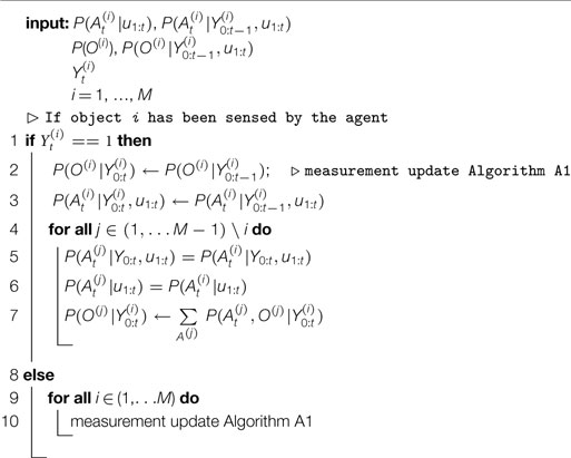
The memory likelihood function’s parameters Ψ_0:t = {(Y_i,l_i)}_i=0:t consist of a set of measurements Y_0:t and offsets l_0:t depicted in greed. The measurements Y_i ∈ {0, 1} are always binary, while the offsets l_i, actions u_t, agent A_t and object O variables’ size are equal to the dimension of the state space. The subscript i of an offset l_i indicates which likelihood function it belongs to. The offset of a likelihood function is given by the summation of all the applied actions from the time the likelihood was added until the current time t, equation (17), which can be computed recursively. The motion update, equation (10), when applied to the joint distribution results in the initial marginal $P\left(A_0;\mathrm{\theta }{}_a^{\ast }\right)$ and the likelihood functions being moved along the agent’s axis. In Algorithm 1, we detail how an action u_t and measurement Y_t, result in the update of the memory likelihood’s parameters from Ψ_0:t−t to Ψ_0:t; this is an implementation of equations (10) and (11).

ALGORITHM 1

ALGORITHM 1. Memory likelihood update

Figure 6 illustrates the evolution of the un-normalized MLMF joint distribution P(A_t, O, Y_0:t|u_1:t), equation (12). For ease of notation, we will omit at times the parameters of the probability functions. Both $P\left(A_0;\mathrm{\theta }{}_a^{\ast }\right)$ and $P\left(O;\mathrm{\theta }{}_o^{\ast }\right)$ were initialized as for the histogram-SLAM example in Figure 5. Two actions u_1:2 = 1 are applied and three measurements Y_0:2 = 0 received which are then integrated into the filter. Since initialization of the joint distribution at t = 0 until t = 2 the object’s marginal $P\left(O;\mathrm{\theta }{}_o^{\ast }\right)$ remains unchanged and the agent’s marginal $P\left(A_2\mathrm{|}{u}_{1:2};\mathrm{\theta }{}_a^{\ast }\right)$ is updated by the two actions according to the motion update, see Figure 6 (Top right). The product of these two marginals (terms of equation (12) before the memory likelihood product) results in the joint probability distribution $P\left(A_2,O\mathrm{|}{u}_{1:2};\mathrm{\theta }{}_a^{\ast },\mathrm{\theta }{}_o^{\ast }\right)$ illustrated in Figure 6 (Middle-right).

FIGURE 6

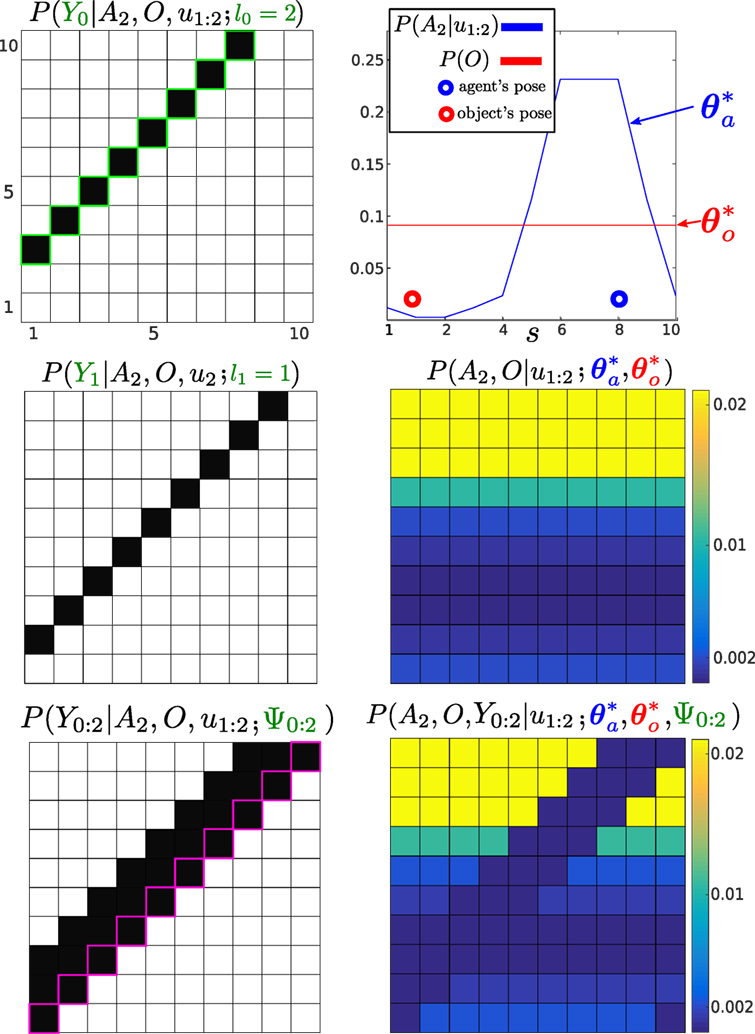
Figure 6. Un-normalized MLMF joint distribution, numerator of equation (12), at time t = 3. Three measurements (all Y = 0) and two actions (both u = 1) have been integrated into the joint distribution, for simplicity we do not consider any motion noise. Left column: the first plot illustrates the likelihood of the first measurement Y₀. We highlight the contour in light-green to indicate that it was the first applied likelihood function (see the correspondence with Figure 5). The first likelihood function has been moved by the 2 actions, the second likelihood function has been moved by one action (the last one, u₂ = 1), and the third likelihood has had no action applied to it yet. The last applied likelihood function is highlighted in pink, and the product of all the likelihoods since t = 0 until t = 3 is depicted at the bottom of the figure, which is P(Y_0:2|A₂, O, u_1:2). Right column: the top figure illustrates the original marginal of the object $P\left(O;\mathrm{\theta }{}_o^{\ast }\right)$, which remains unchanged, and the agent’s marginal $\mathit{\text{P}}\left({\mathit{\text{A}}}_{\text{2}}\mathrm{|}{\mathit{\text{u}}}_{\text{1:2}};\mathrm{\theta }{}_{\mathit{\text{a}}}^{\ast }\right)$, which has moved in accordance to the motion-update function. Their product would result in the joint distribution $\mathit{\text{P}}\left({\mathit{\text{A}}}_{\text{2}},\mathit{\text{O}}\mathrm{|}{\mathit{\text{u}}}_{\text{1:2}};\mathrm{\theta }{}_{\mathit{\text{a}}}^{\ast },\mathrm{\theta }{}_{\mathit{\text{o}}}^{\ast }\right)$ illustrated in the middle figure if evaluated at each state (i, j). The bottom figure is the result of multiplying $\mathit{\text{P}}\left({\mathit{\text{A}}}_{\text{2}},\mathit{\text{O}}\mathrm{|}{\mathit{\text{u}}}_{\mathit{\text{1:2}}};\mathrm{\theta }{}_{\mathit{\text{a}}}^{\ast },\mathrm{\theta }{}_{\mathit{\text{o}}}^{\ast }\right)$ with P(Y_0:2|A₂, O, u_1:2; Ψ_0:2) giving the filtered joint distribution (equation (12)).

In the left column of Figure 6, we illustrate how the memory likelihood term, equation (15), is updated according to Algorithm 1. In the Top left, the first likelihood function $P\left(Y_0\mathrm{|}{A}_2,O,u_{1:2};l_0\right)$ is illustrated. As two actions have been applied, Algorithm 1 is applied twice, which results in an $l_0=2$ parameter for the first likelihood function. In this figure, we highlighted the likelihood in light-green to indicate that it was the first added to the memory term making it convenient to compare to Figure 5. As for the second likelihood function $P\left(Y_1|A_2,O,u_2;l_1\right)$, only one action has been applied and the third likelihood function $P\left(Y_2\mathrm{|}{A}_2,O;l_2=0\right)$ has not yet been updated by the next action. The parameters of the memory likelihood function, equation (15), are: Ψ_0.2 = {(0, 2)_i=0, (0, 1)_i=1, (0, 0)_i=2} and its evaluation is illustrated in the Bottom left of Figure 6.

The reader may have noticed that the amplitude of the values of the filtered joint distribution illustrated in Figure 6 have changed when compared with Figure 5, but not the structure. This is because we have not re-normalized the joint distribution by the evidence P(Y_0:t|u_1:t; α_0:t). We will show in the next section how we can recursively compute the evidence without having to integrate the whole joint distribution, which would be expensive.

Our goal is to be able to compute the marginals P(A_t|Y_0:t, u_1:t; θ_a), P(O|Y_0:t; θ_o) of the agent and object random variables and evidence P(Y_0:t|u_1:t; α_0:t) without having to perform an expensive marginalization over the entire space of the joint distribution as was the case for histogram-SLAM. The next section describes how to efficiently compute the evidence and the marginals. For ease of notation, we will not always show the conditioned actions u_1:t, so P(A_t, O|Y_0:t, u_1:t) will be P(A_t, O|Y_0:t).

3.1. Evidence and Marginals

3.1.1. Evidence

The evidence of the measurement $P\left(Y_{0:t}\mathrm{|}{u}_{1:t};\mathrm{\alpha }{}_{\mathbf{\text{0}}:\mathbf{\text{t}}}\right)$, equation (12), is the amount of probability mass re-normalized to the other parameters of the joint distribution as a result of the consecutive application of the likelihood function. At time step t, the normalizing factor to be added to the evidence is the difference between the probability mass located inside A ∩ O before and after the application of the measurement function P(Y_t|A_t, O), see equations (18) and (19) (see Appendix D for the full derivation)

$\begin{array}{ll}\hfill & {\mathrm{\alpha }}_t={\displaystyle \sum _{A_t}{\displaystyle \sum _O}}\left(\right.P\left(Y_t\mathrm{|}{A}_t,O\right)-1\left)\right.P_{\cap }\left(A_t,O,Y_{0:t-1}\mathrm{|}{u}_{1:t}\right)\end{array}$ (18)

$\begin{array}{ll}\hfill & P\left(Y_{0:t}\mathrm{|}{u}_{1:t};\mathrm{\alpha }{}_{\mathbf{\text{0}}:\mathbf{\text{t}}}\right)=1+\underset{{\mathrm{\alpha }}_{0:t}}{\underbrace{{\mathrm{\alpha }}_{0:t-1}+{\mathrm{\alpha }}_t}}.\end{array}$ (19)

The advantage of equation (18) is that the summation is only over the states that are in the dependent area ∩ of the joint distribution. Until an object is sensed, the likelihood will always be zero P(Y_t|A_t, O) = 0 and α_t will correspond to the probability mass, which falls within the region of the joint distribution in which the likelihood function is zero. As we perform the filtering process, we will never re-normalize the whole joint distribution, but only keep track of how much it should have been normalized. The normalization factor in question will never be negative, as the joint distribution sums to one and each α_t represents some of the mass removed from the joint distribution. Since we keep track of the history of applied measurement likelihood functions the same amount of probability mass is never removed twice from the joint distribution.

3.1.2. Marginals

There are two different sets of marginals used in the MLMF filter. The first set are the joint marginals of the joint distribution, equation (12) parameterized by $\mathrm{\theta }{}_a^{\ast }$ and $\mathrm{\theta }{}_o^{\ast }$. The second set of marginals are the filtered marginals, which are updated by evaluating the joint distribution in dependent states and are parameterized by ${\mathrm{\theta }}_a$ and ${\mathrm{\theta }}_o$. At initialization before the first action or observation is made the parameters of the filtered marginal are set equal to those of the joint distribution. MLMF takes advantage of the sparsity of the likelihood function, which results in only the dependent elements of the marginal being affected, equation (20) (see Appendix E for the full derivation of equation (20))

$\begin{array}{l}\hfill P\left(O\mathrm{|}{Y}_{0:\mathbf{\text{t}}};{\mathrm{\theta }}_o\right)=P\left(O\mathrm{|}{Y}_{0:\mathbf{\text{t}}-\mathbf{\text{1}}};{\mathrm{\theta }}_o\right)-\left(\right.P_{\cap }\left(O\mathrm{|}{Y}_{0:t-1}\right)-{\mathbf{\text{P}}}_{\cap }\left(\mathbf{\text{O}}\mathrm{|}{\mathbf{\text{Y}}}_{\mathbf{\text{0}}:\mathbf{\text{t}}}\right)\left)\right.\end{array}$ (20)

$\begin{array}{llll}\hfill & {\mathbf{\text{P}}}_{\cap }\left(\mathbf{\text{O}}\mathrm{|}{\mathbf{\text{Y}}}_{\mathbf{\text{0}}:\mathbf{\text{t}}};\mathrm{\theta }{}_a^{\ast },\mathrm{\theta }{}_o^{\ast },{\mathrm{\Psi }}_{\mathbf{0:}\mathit{\text{t}}},\mathrm{\alpha }{}_{\mathbf{\text{0}}:\mathbf{\text{t}}}\right)={\displaystyle \sum _{A_t}}{\mathbf{\text{P}}}_{\cap }\left({\mathbf{\text{A}}}_{\mathbf{\text{t}}},\mathbf{\text{O}}\mathrm{|}{\mathbf{\text{Y}}}_{\mathbf{\text{0}}:\mathbf{\text{t}}},{\mathbf{\text{u}}}_{\mathbf{\text{1}}:\mathbf{\text{t}}};\mathrm{\theta }{}_a^{\ast },\mathrm{\theta }{}_o^{\ast },{\mathrm{\Psi }}_{\mathbf{0:}\mathit{\text{t}}},\mathrm{\alpha }{}_{\mathbf{\text{0}}:\mathbf{\text{t}}}\right)& \hfill & \\ \hfill & =\frac{{\displaystyle \sum _{A_t}}{P}_{\cap }\left(O;\mathrm{\theta }{}_o^{\ast }\right)P_{\cap }\left(A_t\mathrm{|}{u}_{1:t};\mathrm{\theta }{}_a^{\ast }\right)P\left(Y_{0:t}\mathrm{|}{A}_t,O,u_{1:t};{\mathrm{\Psi }}_{\mathbf{0:}\mathit{\text{t}}}\right)}{P\left(Y_{0:t}\mathrm{|}{u}_{1:t};\mathrm{\alpha }{}_{\mathbf{\text{0}}:\mathbf{\text{t}}}\right)}.\end{array}$ (21)

Equation (20) is recursive, $P\left(O\mathrm{|}{Y}_{0:\mathbf{\text{t}}};{\mathrm{\theta }}_o\right)$ is computed in terms of $P\left(O\mathrm{|}{Y}_{0:\mathbf{\text{t}}-\mathbf{\text{1}}};{\mathrm{\theta }}_o\right)$. Figure 7 illustrates a measurement update of the MLMF. The illustrated marginals (Bottom row) are (on the left) the joint marginals $P\left(A_t\mathrm{|}{u}_{1:t};\mathrm{\theta }{}_a^{\ast }\right)$, $P\left(O;\mathrm{\theta }{}_o^{\ast }\right)$ and (on the right) the filtered marginals $P\left(A_t\mathrm{|}{Y}_{0:t},u_{1:t};{\mathrm{\theta }}_a\right)$, $P\left(O\mathrm{|}{Y}_{0:t};{\mathrm{\theta }}_o\right)$.

FIGURE 7

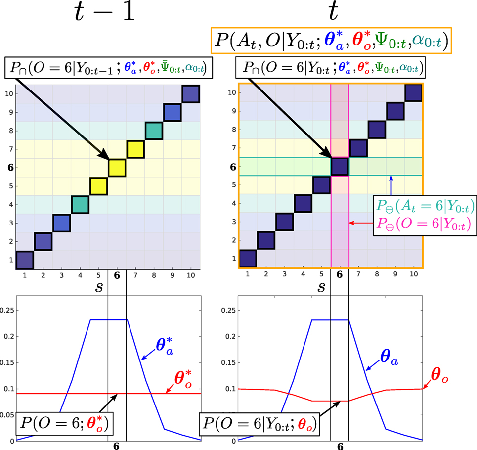
Figure 7. Filtered marginals. Illustration of the agent and object marginal update (equation (20)). The joint distribution parameters that are independent A ⊖ O are pale, and the dependent areas A ∩ O, where P(Y_t < 1|A_t, O), are bright. MLMF only evaluates the joint distribution in dependent states. For each state s of the marginals 1,…, 10, the difference of the marginals inside the dependent area, before and after the measurement likelihood is applied, is evaluated and removed from the marginals P(A_t|Y_0:t−1, u_1:t; θ_a), P(O|Y_0:t−1; θ_o) leading to P(A_t|Y_0:t, u_1:t; θ_a), P(O|Y_0:t; θ_o) (we did not show u_1:t in the figure for ease of notation). Bottom left: joint marginals $\mathit{\text{P}}\left({\mathit{\text{A}}}_{\mathit{\text{t}}}\mathrm{|}{\mathit{\text{u}}}_{\text{1:}t};\mathrm{\theta }{}_{\mathit{\text{a}}}^{\ast }\right)$ and $\mathit{\text{P}}\left(\mathit{\text{O}};\mathrm{\theta }{}_{\mathit{\text{o}}}^{\ast }\right)$ remain unchanged by measurements.

The shape of the joint marginals remain unchanged by measurements during the filtering process, they are the parameters of the joint distribution used to update the filtered marginals. Table 1 summarizes the functions and parameters of the MLMF for two random variables, an agent and object.

TABLE 1

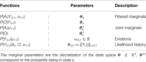
Table 1. MLMF functions with associated parameters.

We evaluated the MLMF with histogram-SLAM in the case of the 1D filtering scenario illustrated in Figure 5, and we found them to be identical. Having respected the formulation of Bayes rule, we assert that the MLMF filtering steps (see Algorithm A1, Appendix A for a more detailed application of motion-measurement update steps) are Bayesian Optimal Filter¹. Next we evaluate both space and time complexity of the MLMF filter.

4. Space and Time Complexity

For discussion purposes, we consider the case of three beliefs, namely, that of the agent and two other objects O⁽¹⁾ and O⁽²⁾, we subsequently generalize. As stated previously, M stands for the number of filtered random variables including the agent, and N is the number of discrete states in the world. In the following section, we compare the space and time complexity of MLMF-SLAM with histogram-SLAM.

4.1. Space Complexity

Figure 8 (Left) illustrates the volume occupied by the joint distribution for a space with N states. Histogram-SLAM would require N³ parameters for the joint distribution P(A, O⁽¹⁾, O⁽²⁾; θ) and 3 N parameters to store the marginals. In general, for M random variables N^M + M N parameters are necessary, giving an exponential space complexity 𝒪(N^M).

FIGURE 8

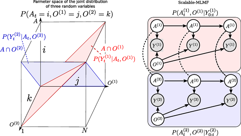
Figure 8. Left: Joint distribution. P(A, O⁽¹⁾, O⁽²⁾) of the agent and two objects (Y_0:t and u_1:t omitted). Each likelihood function, P(Y|A, O⁽¹⁾), P(Y|A, O⁽²⁾) corresponds to a hyperplane in the joint distribution The state space is discretized to N bins giving a potential total of N³ parameters for the joint distribution (Histogram case). Right: Scalable-MLMF. Each agent–object joint distribution pair is modeled independently. For clarity, we have left out the action random variable u that is linked to every agent node. Two joint distributions $\mathit{\text{P}}\left({\mathit{\text{A}}}^{\left(\text{1}\right)},{\mathit{\text{O}}}^{\left(\text{1}\right)}\mathrm{|}{\mathit{\text{Y}}}_{\mathrm{0:}t}^{\left(\text{1}\right)}\right)$ and $\mathit{\text{P}}\left({\mathit{\text{A}}}^{\left(\text{2}\right)},{\mathit{\text{O}}}^{\left(\text{2}\right)}\mathrm{|}{\mathit{\text{Y}}}_{\mathrm{0:}t}^{\left(\text{2}\right)}\right)$ parametrize the graphical model. The dashed undirected lines represent a wanted dependency, if present O⁽¹⁾ and O⁽²⁾ are to be dependent through A. In the standard setting, there will be no exchange of information between the individual joint distributions. However, we demonstrate later on how we perform a one-time transfer of information when one of the objects is sensed.

For MLMF-SLAM, each random variable requires two sets of parameters, θ and $\mathrm{\theta }{}^{\ast }$ (see Table 1). Given M random variables, the initial number of parameters is M(2N). At every time step the likelihood memory function increments by one measurement and offset, (Y_t, l = 0) (Algorithm 1). Given a state space of size N, there can be no more than N different measurement functions (one for each state). In the worst-case scenario, the number of memory likelihood function parameters Ψ_0:t, equation (15), will be N. The total number of parameters is M(2N) + N, which gives a final worst-case space complexity linear in the number of random variables, 𝒪(M N).

4.2. Time Complexity

For histogram-SLAM, the computational cost is equivalent to that of the space complexity, 𝒪(N^M), since every state in the joint distribution has to be summed to obtain all the marginals.

For MLMF-SLAM, every state in the joint distribution’s state space that has been changed by the likelihood function has to be summed, see Figure 7. As a result, the computational complexity is directly related to the number of dependent states |A ∩ O|. In Figure 7, this corresponds to states where i = j and there are N out of a total N² states for that joint distribution. Figure 8 (Left) illustrates a joint distribution with N³ states. The dependent states |A ∩ O⁽¹⁾ ∩ O⁽²⁾| are those which are within the blue and red planes (where the likelihood evaluates to zero) and comprise N² states each, giving a total of 2N² − N dependent states (negative is to remove the states we count twice at the intersection of the blue and red plane).

The likelihood term P(Y_t|A_t, O⁽¹⁾) evaluates states to zero, which satisfies (i = j, ∀k), as the measurement of object O⁽¹⁾ is independent of object O⁽²⁾. With 3 objects, the joint distribution would be P(A_t = i, O⁽¹⁾ = j, O⁽²⁾ = k, O^(l) = l) then the likelihood P(Y_t|A_t, O⁽¹⁾) evaluated to zero for (i = j, ∀k, ∀l) which would mean N³ dependent states. In general, for M random variables the computational cost is (M − 1) N^M−1 which gives 𝒪(N^M−1) as opposed to the histogram-SLAM’s 𝒪(N^M). The computation complexity in this setup is still exponential but to the order M − 1 as opposed to M, which nevertheless quickly limits the scalability as more objects are added.

Computing the value of a dependent state (i, j, k) in the joint distribution required evaluating equation (12), which contains a product of N likelihood functions, in the worst-case scenario. However, the likelihood functions are not overlapping and binary. As a result, the complete product does not have to be evaluated since only one likelihood function will affect the state (i, j, k). Thus, evaluating equation (12) yields a cost of 𝒪(1).

5. Scalable Extension to Multiple Objects

To make the MLMF filter scalable, we introduce an independence assumption between the objects and model the joint distribution (equation (22)) as a product of agent–object joint distributions:

$P\left(A_t,o^{\left(1\right)},\cdots ,O^{\left(M-1\right)}\mathrm{|}{Y}_{0:t},u_{1:t}\right)={\displaystyle \prod _{i=1}^{M-1}}P\left(A_t^{\left(i\right)},O^{\left(i\right)}\mathrm{|}{Y}_{0:t}^{\left(i\right)},u_{1:t}\right).$ (22)

The measurement variable Y_t, is the vector of all agent–object measurements, $Y_t={\left[Y_t^{\left(1\right)},\dots ,Y_t^{\left(M-1\right)}\right]}^{\text{T}}$. Each agent–object joint distribution has its own parametrization of the agent’s marginal, $A_t^{\left(1\right)},\dots ,A_t^{\left(M-1\right)}$ which combine to give the overall marginal of the agent A_t. The computation of each object marginal $P\left(O^{\left(i\right)}\mathrm{|}{Y}_{0:t}^{\left(i\right)}\right)$ is independent of the other objects. This is evident from the marginalization, see equations (23) and (24)

$\begin{array}{l}\hfill P\left(O^{\left(i\right)}\mathrm{|}{Y}_{0:t}^{\left(i\right)},u_{1:t}\right)={\displaystyle \sum _{A_t^{(i)}}}P\left(A_t^{\left(i\right)},O^{\left(i\right)}\mathrm{|}{Y}_{0:t}^{\left(i\right)},u_{1:t}\right)\end{array}$ (23)

$\begin{array}{l}\hfill P\left(A_t\mathrm{|}{Y}_{0:t},u_{1:t}\right)={\displaystyle \prod _{i=1}^{M-1}}P\left(A_t^{\left(i\right)}\mathrm{|}{Y}_{0:t}^{\left(i\right)},u_{1:t}\right).\end{array}$ (24)

The independence assumption will create an unwanted effect with respect to agent’s marginal P(A_t|Y_0:t, u_1:t). At initialization the agent marginals should be equal, $P\left(A_0\mathrm{|}{Y}_0\right)=P\left(A_0^{\left(i\right)}\mathrm{|}{Y}_0^{\left(i\right)}\right){\forall }_i$; however, this is not the case because of equation (24). To overcome this, we define the marginal, P(A_t|Y_0:t, u_1:t), of the agent as being the average of all the individual pairs $P\left(A^{\left(i\right)}\mathrm{|}{Y}_{0:t}^{\left(i\right)},u_{1:t}\right)$

$P\left(A_t\mathrm{|}{Y}_{0:t},u_{1:t}\right):=\frac{1}{M-1}{\displaystyle \sum _{i=1}^{M-1}}P\left(A_t^{\left(i\right)}\mathrm{|}{Y}_{0:t}^{\left(i\right)},u_{1:t}\right).$ (25)

Figure 8 (Right) depicts the graphical model of the scalable formulation. As each joint distribution pair has its own parametrization of the agent’s marginal and these do not subsequently get updated by one another, the information gained by one joint distribution pair is not transferred. A solution is to transfer information between the marginals A⁽ⁱ⁾ at specific intervals namely when one of the objects is sensed by the agent.

The exchange of information of one joint distribution to another is achieved through the agent’s marginals A⁽ⁱ⁾ according to Algorithm A2, Appendix B. The measurement update is the same as previously described in Algorithm A1 in the case of no positive measurements of the objects. If the agent senses an object, all of the agent marginals of the remaining joint distributions are set to the marginal of the joint distribution pair belonging to the positive measurement $Y_t^{\left(i\right)}$.

Figure 9 depicts the process of information exchange between object O⁽¹⁾ and O⁽²⁾ in the event that the agent senses O⁽²⁾. Prior to the positive detection, both marginals $P\left(A_t^{\left(1\right)}\mathrm{|}{Y}_{0:t-1}^{\left(1\right)},u_{1:t}\right)$ and $P\left(A_t^{\left(2\right)}\mathrm{|}{Y}_{0:t-1}^{\left(2\right)},u_{1:t}\right)$ occupy the same region and are identical. When the agent senses O⁽²⁾ the line defined by the measurement likelihood function $P\left(Y_t^{\left(2\right)}|A_t^{\left(2\right)},O^{\left(2\right)}\right)$ becomes a hard constraint implying that both the agent and O⁽²⁾ have to satisfy this constraint. Figure 10 shows marginals at initialization, prior contact between the agent and object and the after the measurement (post contact) has been integrated into the marginals (resulting from the joint distributions in Figure 9).

FIGURE 9

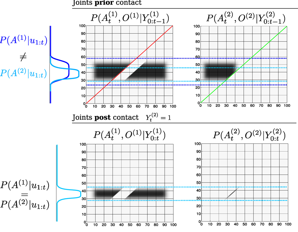
Figure 9. Transfer of information (joint distributions). Top: joint distributions of $\mathit{\text{P}}\left({\mathit{\text{A}}}_{\mathit{\text{t}}}^{\left(\text{1}\right)},{\mathit{\text{O}}}^{\left(\text{1}\right)}\mathrm{|}{\mathit{\text{Y}}}^{\left(\text{1}\right)}\right)$ and $\mathit{\text{P}}\left({\mathit{\text{A}}}_{\mathit{\text{t}}}^{\left(\text{2}\right)},{\mathit{\text{O}}}^{\left(\text{2}\right)}\mathrm{|}{\mathit{\text{Y}}}^{\left(\text{2}\right)}\right)$ prior sensing, ${\mathit{\text{Y}}}_{\mathit{\text{t}}}^{\left(\text{2}\right)}=\text{1}$, see Figure 10 (Top right) for the corresponding marginals. The red and green lines across the joint distributions correspond to the region in which the likelihood functions $\mathit{\text{P}}\left({\mathit{\text{Y}}}_{\mathit{\text{t}}}^{\left(\text{1}\right)}\mathrm{|}{\mathit{\text{A}}}_{\mathit{\text{t}}}^{\left(\text{1}\right)},{\mathit{\text{O}}}^{\left(\text{1}\right)}\right)$ and $\mathit{\text{P}}\left({\mathit{\text{Y}}}_{\mathit{\text{t}}}^{\left(\text{2}\right)}\mathrm{|}{\mathit{\text{A}}}_{\mathit{\text{t}}}^{\left(\text{2}\right)},{\mathit{\text{O}}}^{\left(\text{2}\right)}\right)$ will change the joint distributions. The dotted blue lines are to ease the comparison of the joint distributions prior and post sensing. Bottom right: After the agent has sensed O⁽²⁾, all the probability mass that was not overlapping the green line becomes an infeasible solution to the agent and object locations. At this point the marginals $\mathit{\text{P}}\left({\mathit{\text{A}}}_{\mathit{\text{t}}}^{\left(\text{1}\right)}\mathrm{|}{\mathit{\text{u}}}_{\text{1:}t}\right)\ne \mathit{\text{P}}\left({\mathit{\text{A}}}_{\mathit{\text{t}}}^{\left(\text{2}\right)}\mathrm{|}{\mathit{\text{u}}}_{\text{1:}t}\right)$ are no longer equal (see the blue marginals Top). Bottom left: The constraint imposed by the likelihood function of the second object (green line) is transferred to the joint distribution of the first object according to Algorithm A2. This results in a change in the joint distribution $\mathit{\text{P}}\left({\mathit{\text{A}}}_{\mathit{\text{t}}}^{\left(\text{1}\right)},{\mathit{\text{O}}}^{\left(\text{1}\right)}\mathrm{|}{\mathit{\text{Y}}}^{\left(\text{1}\right)}\right)$, which satisfies the constraints imposed by the agent’s marginal from the joint distribution $\mathit{\text{P}}\left({\mathit{\text{A}}}_{\mathit{\text{t}}}^{\left(\text{2}\right)},{\mathit{\text{O}}}^{\left(\text{2}\right)}\mathrm{|}{\mathit{\text{Y}}}^{\left(\text{2}\right)}\right)$.

FIGURE 10

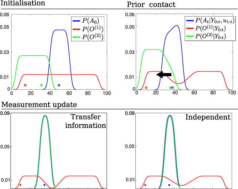
Figure 10. Transfer of information (marginals). Top left: Initial beliefs of the agent and object’s location. The agent moves to the left until it senses object O⁽²⁾. Top right: Marginals prior the agent entering in contact with the green object, see Figure 9 (Top) for an illustrate of the joint distributions. Bottom left: resulting marginals after setting the agent marginals of each joint distribution equal ${\mathit{\text{A}}}_{\mathit{\text{t}}}^{\left(\text{1}\right)}={\mathit{\text{A}}}_{\mathit{\text{t}}}^{\left(\text{2}\right)}$ according to Algorithm A2. The object marginal $P\left(O^{\left(2\right)}\mathrm{|}{Y}_{0:t}\right)$ is recomputed. Bottom Right: resulting marginals in which the objects have no influence on one another. Note that a transfer of information has caused a change in the marginal O⁽¹⁾.

The result of introducing a dependency between the objects through the agent’s marginals in the event of a sensing and treating them independently gives the same solution as the histogram filter in this particular case. However, as each individual marginal $A_t^{\left(i\right)}$ diverges from the other marginals, the filtered solution will diverge from the histogram’s solution. We assume, however, that the objects are weakly dependent and sharing information during positive sensing events is sufficient. In section 6.2, we will evaluate the independence assumption with respect to the histogram filter. Table 2 summarizes the time and space complexity for the three filters.

TABLE 2

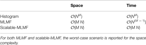
Table 2. Time and space complexity summary.

6. Evaluation

We conduct three different types of evaluation to quantify the scalability and correctness of the scalable-MLMF filter. The first experiment tests the scalability of our filter in terms of processing time taken per motion-measurement update cycle. The second experiment evaluates the independence assumption made in the scalable-MLMF filter between the objects. The third and final experiment determines the effect of the memory size on a search policy to locate all the objects in the Table world.

6.1. Evaluation of Time Complexity

We measured the time taken by the motion-measurement update loop, as a function of the number beliefs and number of states per belief. We started with 100 states per belief and gradually increase it to 10,000,000 over 50 steps. Each of the 50 steps treated 2–25 objects. Figure 11 (Left) illustrates the computational cost as a function of number of states and objects. For each state-object pair 100, motion-measurement updates were performed. Most of the trials returned time updates below 1 Hz. Figure 11 (Right) shows the computational cost as a function of the number of states plotted for 6 different filter runs with a different number of objects. As the number of states increases exponentially so does the computational cost. Note the cost increases at the same rate as the number of states, which increase at a rate exponential in the number of random variables, meaning that the computational complexity is linear with respect to the number of states. This result is in agreement with the asymptotic time complexity.

FIGURE 11

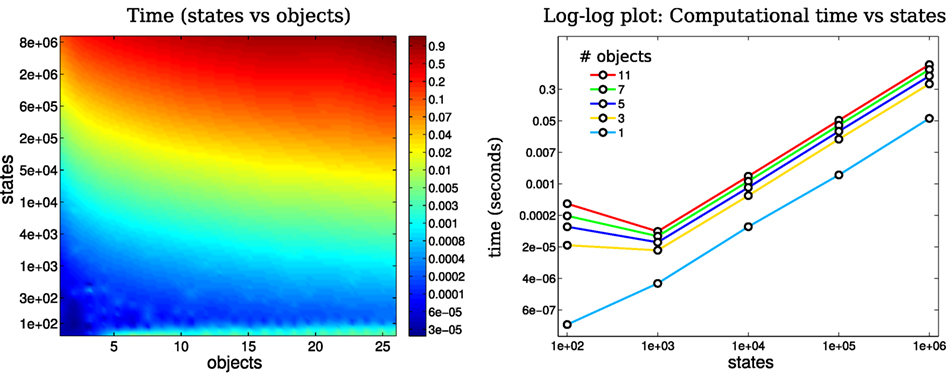
Figure 11. Time complexity: Left: mean time taken for a loop update (motion and measurement) as a function of the number of states in a marginal and the number of objects present. Right: Log–log plot of time taken for a loop update with respect to the number of states in the marginal. The color coded lines are associated with the number of objects present. As the number of states increases exponentially the computational cost matches it.

6.2. Evaluation of the Independence Assumption

In section 5, we made the assumption (for scalability reasons) that the objects’ beliefs are independent of one another. This assumption is validated by comparing the MLMF filter on three random variables, an agent and two objects, with the ground truth, which we obtain from the standard histogram filter. For each of the three beliefs (the agent and two objects), 100 different marginals were generated and the true locations (actual position of the agent and objects) were sampled. Figure 12 (Top left) illustrates one instance of the initialization of the agent and object marginals with their associated sampled true position. The agent carries out a sweep of the state space for each of the marginals and the policy is saved and run with the scalable-MLMF filter. In the first experiment, we assumed that the objects are completely independent and that there was no transfer of information between the pair-wise joint distributions. In the second and third experiments, there is an exchange of information as described in Algorithm A2. Here, we compare the effect of using the product of the agent’s marginals, equation (24), with the average of the marginals, equation (25). We expect the average of the agent’s marginal to yield a result closer to the ground truth as the marginal of the agent P(A_t|Y_0:t, u_1:t) at initialization is the same as the ground truth (the histogram-SLAM’s). As for the marginal of the objects P(O⁽ⁱ⁾|Y_0:t), we expect the difference between them to be independent of whether the product or average of the agent’s marginal is used. This results from Algorithm A2. When an object i is sensed all the corresponding agent marginals P(A^(j)|u_1:t) are set equal to P(A⁽ⁱ⁾|u_1:t) and not to P(A_t|Y_0:t, u_1:t). This is a design decision of our information transfer heuristic. There are many other possibilities but this is one of the simplest. For each of the 100 sweeps, the ground truth is compared with the scalable-MLMF using the Hellinger distance (equation (26))

$H\left(P,Q\right)=\frac{1}{\sqrt{2}}∥\sqrt{P}-\sqrt{Q}{∥}_2$ (26)

which is a metric that measures the distance between two probability distributions. Its value lies strictly between 0 (the two distributions are identical) and 1 (no overlap between them). Figure 12 shows the kernel density distribution of the Hellinger distances taken at each time step for all 100 sweeps. In the Top left of the figure, for the case when no transfer of information is a applied, all the marginals are far from the ground truth. This results from the introduction of the independence assumption, necessary to scale the MLMF. Figure 12 (Bottom) shows the results for difference between the product and average of the agents marginals. As expected, there is no difference between the objects’ marginals when considering both methods (product and average) with respect to the ground truth. The predominant difference occurs in the agent’s marginal P(A_t|Y_0:t, u_1:t). This is also expected and prompted the introduction of the average method instead of the product.

FIGURE 12

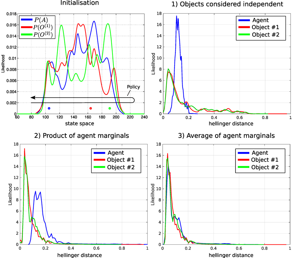
Figure 12. Comparison of scalable-MLMF and the histogram filter. A deterministic sweep policy was carried out for 100 different initializations of the agent and object beliefs. Top left: one particular Initialization of the agent and object random variables. The true position of the agent and objects was sampled at random. The black arrow indicates the general policy, which was followed for each of the 100 sweeps. These were performed for (1) scalable-MLMF with objects considered to be independent at all times (Algorithm A2). (2) Agent marginal P(A_t|Y_0:t, u_1:t) is the product of marginals $\mathit{\text{P}}\left({\mathit{\text{A}}}_{\mathit{\text{t}}}^{\left(\mathit{\text{i}}\right)}\mathrm{|}{\mathit{\text{Y}}}_{\mathrm{0:}t}^{\left(\mathit{\text{i}}\right)},{\mathit{\text{u}}}_{\text{1:}t}\right)$, equation (24). (3) Marginal P(A_t|Y_0:t, u_1:t) is taken to be the average of all marginals $\mathit{\text{P}}\left({\mathit{\text{A}}}_{\mathit{\text{t}}}^{\left(\mathit{\text{i}}\right)}\mathrm{|}{\mathit{\text{Y}}}_{\mathrm{0:}t}^{\left(\mathit{\text{i}}\right)},{\mathit{\text{u}}}_{\text{1:}t}\right)$, equation (25). For each of these three experiments, we report the kernel density estimation over the Hellinger distances taken at every time step between ground truth (from histogram filter) and scalable-MLMF.

The scalable-MLMF information exchange heuristic will not lead to any of the objects marginals probability mass being falsely removed during the information transfer, which is close to a winner-take-all approach in terms of beliefs. When object i is sensed its associated agent marginal is set to all other agent–object joint pairs, which results in the information accumulated in the jth agent marginals being replaced by the ith.

6.3. Evaluation of Memory

The memory measurement likelihood function P(Y_0:t|A_t, O, u_1:t; Ψ_0:t) is parameterized by the history of all the measurement likelihood functions that have been applied to the joint distribution since initialization. As detailed earlier, there can be no more than |Ψ_0:t| ≤ N different measurement likelihood functions added to memory. In the case of a very large state space, this might be cumbersome. We investigate how restricting the memory size, the number of parameters |Ψ_0:t|, can impact on the decision process in an Active-SLAM setting. Given our setup, a breadth-first search in the action space is chosen with a one-time step horizon, making it a greedy algorithm. The objective function utilized is the information gain of the beliefs after applying an action (equation (27))

$\begin{array}{l}\hfill u_t={\text{arg\hspace{0.17em}max}}_{u_t}H\left\{P\left(A_{t-1},O\mathrm{|}{Y}_{0:t-1},u_{1:t-1}\right)\right\}-{\mathbb{E}}_{Y_t}\left[H\left\{P\left(A_t,O\mathrm{|}{Y}_{0:t},u_{1:t}\right)\right\}\right].\end{array}$ (27)

For each action the filter is run forward in time and all future measurements since we cannot know ahead of time the actual measurement. The information gain is the difference between the current entropy (defined by H{⋅}) and the future entropy after the simulated motion and measurement update. The action with the highest information gain is subsequently selected. This is repeated at each time step. Figure 13 illustrates the environment setup for a 1D and 2D case. The agent’s task is to find the objects in the environment.

FIGURE 13

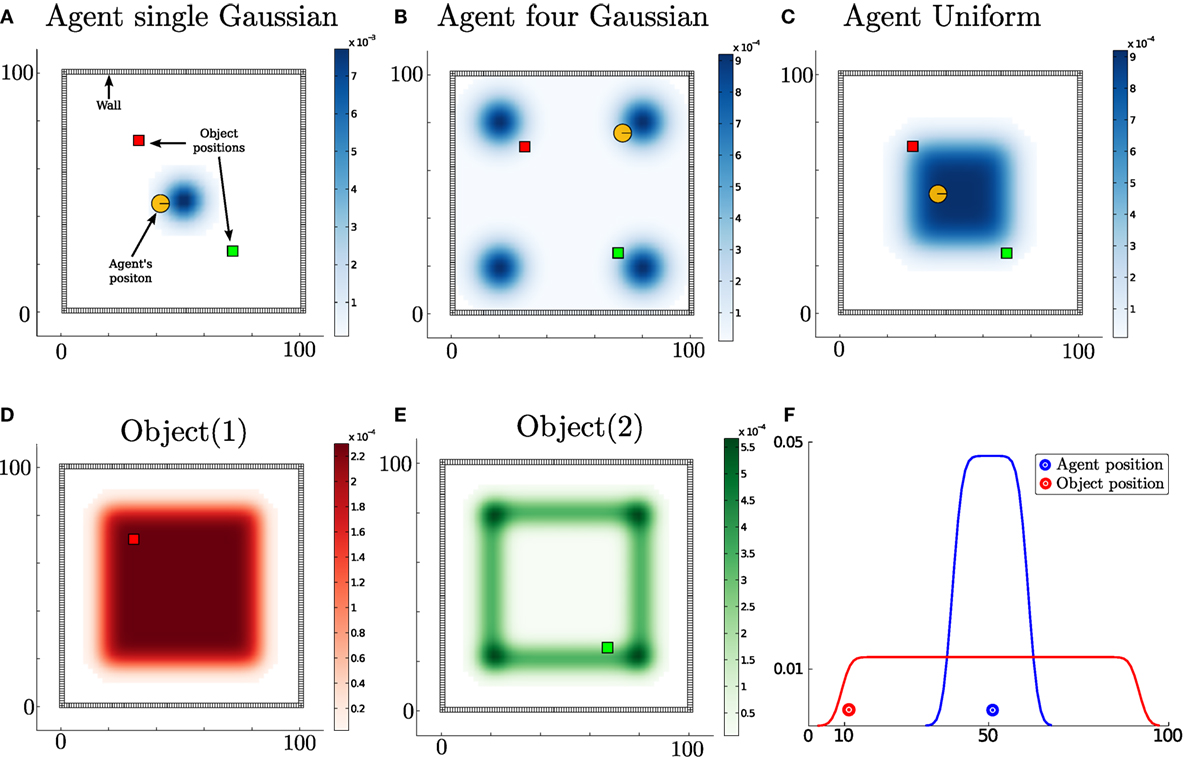
Figure 13. Agent’s prior beliefs. Two types of environment, the first is a 2D world where the agent lives in a square surrounded by a wall while the second is a 1D world. In the 2D figures, the agent is illustrated by a circle with a bar to indicate its heading. The true location of the objects is represented by color coded squares. Top row, (A–C) three different initializations of the agent’s location. Bottom row, (D) the agent’s prior beliefs with respect to the location of the first object and (E) belief of the second object’s location. Bottom row, (F) 1D world with one object.

For the 2D search, we consider three different initializations (single-Gaussian, four-Gaussian, Uniform) for the agent’s belief where there are two objects to be found. Ten searches are carried out for each of the three initializations of the agent’s beliefs. The agent’s true location, for each search, is sampled from its initial belief, and the objects’ locations (red and green squares in Figure 13) are kept fixed throughout all searches. Each search is repeated for 18 different memory sizes ranging from 1 to N (the number of states). For the 1D search case, one object is considered since adding more objects makes the search easier and the interest lies in the memory effects of the search and not the search itself. In Figures 14 and 15, we report on the time taken to find all objects with respect to a given memory size, which is shown as the percentage of the total number of states. In the 1D search case, the time variability taken to find the object converges when the memory size is at 60% of the original state space. As for the 2D search with 2 beliefs (agent and 1 object), the convergence depends on the agent’s initial belief. For the 1-Gaussian (green line), all searches take approximately the same amount of time after a memory size of 9%. As for the remaining two initializations, convergence is achieved at 48%. The same holds true for the case of 3 beliefs (agent and 2 objects).

FIGURE 14

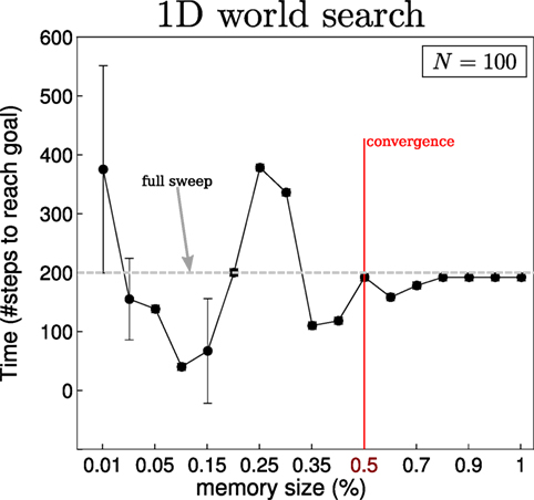
Figure 14. Memory size vs time to find object in 1D. Results of the effect of the memory size on the decision process for the 1D search illustrated in Figure 13F. The memory size is reported as the percentage of total number of states present in the marginal space. At 100%, the size of the memory is equal to that of the state space, N = 100 in this case. A total sweep of the entire state space would result in a total of 200 steps, the dotted gray line in the figure. When no restrictions are placed on the memory size, the policy following the greedy approach takes around 180 steps. This result converges when the number of parameters |Ψ_0:t| of the memory likelihood function is greater than 50% of the original state space.

FIGURE 15

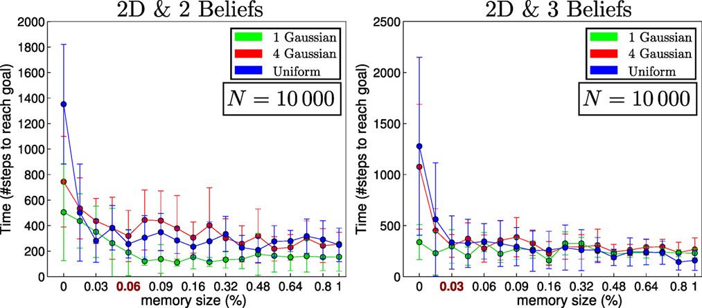
Figure 15. Memory size vs time to find objects in 2D. The initial beliefs correspond to those of Figure 13A for Gaussian (green line), Figure 13B for 4 Gaussians (red line), and Figure 13C for uniform (blue line), both objects are initialized according to Figures 13D,E.

In the 2D searches, the memory size has a less impact on the time taken to find the objects than in the 1D (which is a special search case). Only when the memory size is less than 6% is there a significant change. We conclude that at least in the case of the greedy one-step look-ahead planner that is frequently used in the literature, the size of the memory seems not to be a limiting factor in terms of the time taken to accomplish the search.

7. Conclusion

This work addresses the Active-SLAM filtering problem for scenarios in which sensory information relating to the map is very limited. Current SLAM algorithms filter the errors originating from sensory measurements and not prior uncertainty. By making the assumption that the joint distribution of all the random variables is a multivariate Gaussian, inference is tractable. Since the origin of the uncertainty does not originate from the measurement noise, no assumption can be made about the structure of the joint distribution. In this case, a suitable filter would be the histogram, which makes no assumption about the shape or form taken by the joint distribution. However, the space and time complexity are exponential with respect to the number random variables, and this is a major limiting factor for scalability.

The main contribution of this work is a formulation of a histogram Bayesian state space estimator in which the computational complexity is both linear in time and space. A different approach to other SLAM formulations as been taken in the sense that the joint distribution is not explicitly parameterized avoiding the exponential increase in parameter space, which would otherwise have been the case. The MLMF parameters consist of the marginals and the history of measurement functions, which have been applied. By solely evaluating the joint distribution at the states that are affected by the current measurement function while taking into account the memory, the MLMF filter obtains the same filtered marginals as the histogram filter. Further, the worst-case space complexity is linear rather than exponential, and the time complexity remains exponential but increases at lower rate than in the histogram filter. In striving to make the filter scalable, we make the assumption that the objects are independent. An individual MLMF is used for each agent–object pair. We evaluate the difference between the scalable-MLMF with a ground truth provided by the histogram filter for 100 different searches with respect to the Hellinger distance. We conclude that the divergence is relatively small and thus the scalable-MLMF filter provides a good approximation to the true filtered marginals. We evaluate the time taken to perform a motion-update loop for different discretizations of the state space (100–10,000,000 states) and number of objects (2–25). In most of the cases, we achieve an update cycle rate below 1 Hz. We evaluate how the increase of the number of states affects the computational cost and find the relationship to be linear and thus in agreement with our analysis of the asymptotic growth rate. We analyze the effect of the memory size (the remembered number of measurement likelihood functions) on the decision-theoretic process of reducing the uncertainty of the map and agent during a search task. We conclude that in the 2D case the memory size has much less effect than in the 1D case and that it is unnecessary to remember every single measurement function.

This implies that the MLMF and scalable-MLMF that we have are a computationally tractable means of performing SLAM in a case scenario in which mostly negative information is present and the joint distribution cannot be assumed to have any specific structure. Furthermore, the filter can be used at a higher cognitive level than the processing of raw sensory information as is often the case in Active-SLAM. MLMF would be well suited for reasoning tasks where the robot’s field of view is limited.

An interesting future extension could be to make the original MLMF filter scalable without introducing assumptions. One possibility could to be to consider Monte Carlo integration methods for inference. These can scale well to high dimensional spaces while still providing reliable estimates. A second possibility could be to investigate the use of Gaussian Mixtures as a form of parameterization of the marginals to blend our filter with EKF-SLAM. This would allow the parameters to grow quadratically with respect to the dimension of the marginal space as opposed to exponentially as is the case with the histogram and MLMF filters.

Author Contributions

GC: theory, implementation, analysis, and wrote manuscript. AB: guidance on theory and manuscript.

Conflict of Interest Statement

The authors declare that the research was conducted in the absence of any commercial or financial relationships that could be construed as a potential conflict of interest.

Supplementary Material

The Supplementary Material for this article can be found online at https://www.frontiersin.org/article/10.3389/frobt.2017.00040/full#supplementary-material.

Video S1. Top left : initial marginals, the blue and red probability density functions (solid red and blue) represent the belief the agent has of his position and that of the object being searched. Bottom right: product of the original marginals (dashed blue and red in top left figure) and the current likelihood function. Bottom left: the memory likelihood functions (equation (15)) which is the product of all likelihood functions. Top right: the joint distribution, which is result of the product of both functions in the bottom figures. The marginalization of the joint distribution would result in solid blue and red marginals, depicted in the top left figure. The marginalization is computed at each step along the pink line illustrated in the bottom right figure. This avoids performing an expensive margnisalization over the entire joint distribution.

Video S2. 2D search example of an experiment illustrated in Figure 13. The agent has to locate the red square. As the agent reduces his uncertainty by using the wall, this propegates to the entire object marginal (shown in red).

Video S3. 2D search example of an experiment illustrated in Figure 13. The agent must locate two objects (red and green). When the agent locates the red object, their marginals become the same, as both of them have to be located at the same point.

Footnote

1. ^An optimal Bayesian solution is an exact solution to the recursive problem of calculating the exact posterior density (Arulampalam et al., 2002).

References

Arulampalam, M., Maskell, S., Gordon, N., and Clapp, T. (2002). A tutorial on particle filters for online nonlinear/non-Gaussian Bayesian tracking. Trans. Sig. Process. 50, 174–188. doi: 10.1109/78.978374

CrossRef Full Text | Google Scholar

Bailey, T., Nieto, J., and Nebot, E. (2006). “Consistency of the FastSLAM algorithm,” in International Conference on Robotics and Automation (ICRA), Sydney, 424–429.

Google Scholar

Bake, C., Tenenbaum, J., and Saxe, R. (2011). Bayesian theory of mind: modeling joint belief-desire attribution. J. Cognit. Sci. 33, 2469–2474.

Google Scholar

Cadena, C., Carlone, L., Carrillo, H., Latif, Y., Scaramuzza, D., Neira, J., et al. (2016). Past, present, and future of simultaneous localization and mapping: towards the robust-perception age. Trans. Robot. 32, 13091332. doi:10.1109/TRO.2016.2624754

CrossRef Full Text | Google Scholar

de Chambrier, G., and Billard, A. (2013). “Learning search behaviour from humans,” in International Conference on Robotics and Biomimetics (ROBIO), Shenzhen, 573–580.

Google Scholar

Durrant-Whyte, H., and Bailey, T. (2006). Simultaneous localisation and mapping (SLAM): part I the essential algorithms. Robot. Automat. Mag. 13, 99–110. doi:10.1109/mra.2006.1638022

CrossRef Full Text | Google Scholar

Engel, J., Schöps, T., and Cremers, D. (2014). “LSD-SLAM: large-scale direct monocular SLAM,” in European Conference on Computer Vision (ECCV), Zurich.

Google Scholar

Grisetti, G., Kummerle, R., Stachniss, C., and Burgard, W. (2010). A tutorial on graph-based slam. IEEE Intell. Transp. Syst. Mag. 2, 31–43. doi:10.1109/MITS.2010.939925

CrossRef Full Text | Google Scholar

Hesch, J., Kottas, D., Bowman, S., and Roumeliotis, S. (2014). Consistency analysis and improvement of vision-aided inertial navigation. Trans. Robot. 30, 158–176. doi:10.1109/TRO.2013.2277549

CrossRef Full Text | Google Scholar

Hidalgo, F., and Brunl, T. (2015). “Review of underwater slam techniques,” in 2015 6th International Conference on Automation, Robotics and Applications (ICARA), Queenstown, 306–311.

Google Scholar

Hoffman, J., Spranger, M., Gohring, D., and Jungel, M. (2005). “Making use of what you don’t see: negative information in Markov localization,” in International Conference on Intelligent Robots and Systems (IROS), Chicago, 2947–2952.

Google Scholar

Hoffmann, J., Spranger, M., Gohring, D., Jungel, M., and Burkhard, H.-D. (2006). “Further studies on the use of negative information in mobile robot localization,” in International Conference on Robotics and Automation (ICRA), Orlando, 62–67.

Google Scholar

Huang, G., Mourikis, A., and Roumeliotis, S. (2013). A quadratic-complexity observability-constrained unscented Kalman filter for SLAM. Trans. Robot. 29, 1226–1243. doi:10.1109/TRO.2013.2267991

CrossRef Full Text | Google Scholar

Ila, V., Polok, L., Solony, M., and Svoboda, P. (2017). Slam++ – a highly efficient and temporally scalable incremental slam framework. Int. J. Robot. Res. 36, 210–230. doi:10.1177/0278364917691110

CrossRef Full Text | Google Scholar

Kuemmerle, R., Grisetti, G., Strasdat, H., Konolige, K., and Burgard, W. (2011). “g2o: A general framework for graph optimization,” in International Conference on Robotics and Automation (ICRA), Shanghai, 3607–3613.

Google Scholar

Li, M., and Mourikis, A. I. (2013). High-precision, consistent EKF-based visual-inertial odometry. Int. J. Robot. Res. 32, 690–711. doi:10.1177/0278364913481251

CrossRef Full Text | Google Scholar

Montemerlo, M., and Thrun, S. (2003). “Simultaneous localization and mapping with unknown data association using FastSLAM,” in International Conference on Robotics and Automation (ICRA), Vol. 2. Acapulco, 1985–1991.

Google Scholar

Montemerlo, M., Thrun, S., Koller, D., and Wegbreit, B. (2003). “FastSLAM 2.0: an improved particle filtering algorithm for simultaneous localization and mapping that provably converges,” in International Conference on Artificial Intelligence (IJCAI), Taipei, 1151–1156.

Google Scholar

Mourikis, A., and Roumeliotis, S. (2007). “A multi-state constraint Kalman filter for vision-aided inertial navigation,” in International Conference on Robotics and Automation (ICRA), Roma, 3565–3572.

Google Scholar

Mur-Artal, R., Montiel, J. M. M., and Tards, J. D. (2015). ORB-SLAM: a versatile and accurate monocular slam system. Trans. Robot. 31, 1147–1163. doi:10.1109/TRO.2015.2463671

CrossRef Full Text | Google Scholar

Mur-Artal, R., and Tardos, J. (2016). ORB-SLAM2: An Open-Source SLAM System for Monocular, Stereo and RGB-D Cameras. (New York: IEEE) CoRR abs/1610.06475.

Google Scholar

Paull, L., Saeedi, S., Seto, M., and Li, H. (2014). AUV navigation and localization: a review. J. Oceanic Eng. 39, 131–149. doi:10.1109/JOE.2013.2278891

CrossRef Full Text | Google Scholar

Paz, L. M., Tards, J. D., and Neira, J. (2008). Divide and conquer: EKF slam in o(n). Trans. Robot. 24, 1107–1120. doi:10.1109/TRO.2008.2004639

CrossRef Full Text | Google Scholar

Plagemann, C., Kersting, K., Pfaff, P., and Burgard, W. (2007). “Gaussian beam processes: a nonparametric Bayesian measurement model for range finders,” in Proceedings of Robotics: Science and Systems (RSS), Philadelphia.

Google Scholar

Rublee, E., Rabaud, V., Konolige, K., and Bradski, G. (2011). “ORB: an efficient alternative to sift or surf,” in International Conference on Computer Vision (ICCV), Barcelona, 2564–2571.

Google Scholar

Thrun, S. (2002). “Particle filters in robotics,” in Annual Conference on Uncertainty in AI (UAI), Alberta, 17.

Google Scholar

Thrun, S., Burgard, W., and Fox, D. (2005). Probabilistic Robotics (Intelligent Robotics and Autonomous Agents). The MIT Press.

Google Scholar

Thrun, S., and Leonard, J. J. (2008). “Simultaneous localization and mapping,” in Springer Handbook of Robotics, eds B. Siciliano and O. Khatib (New York: Springer-Verlag), 871–889.

Google Scholar

Thrun, S., Liu, Y., Koller, D., Ng, Y., Ghahramani, Z., and Durrant-Whyte, H. (2004). Simultaneous localization and mapping with sparse extended information filters. Int. J. Robot. Res. 23.

Google Scholar

Wan, E., and Van Der Merwe, R. (2000). The Unscented Kalman Filter for Nonlinear Estimation. Lake Louise: IEEE, 153–158.

Google Scholar

Appendix

A. MLMF Algorithm

ALGORITHM A1

ALGORITHM A1. MLMF-SLAM

B. Scalable-MLMF Algorithm

ALGORITHM A2

ALGORITHM A2. Scalable-MLMF: Measurement Update

C. Recursion Example

Derivation of the filtered joint distribution, P(A_t, O, Y_t|Y_0:t, u_1:t), for two updates. At initialization when no action has yet been taken the filtered joint distribution is the product of the initial marginals and first likelihood function:

$P\left(A_0,O,Y_0\right)=P\left(O\right)P\left(A_0\right)P\left(Y_0\mathrm{|}{A}_0,O\right).$ (A1)

The first action, u₁ is applied, which to get the filtered joint distribution is marginalized:

$\begin{array}{l}\hfill P\left(A_1,O,Y_0\mathrm{|}{u}_1\right)=P\left(O\right){\displaystyle \sum _{A_0}}P\left(A_1\mathrm{|}{A}_0,u_1\right)P\left(A_0\right)P\left(Y_0\mathrm{|}{A}_0,O\right)\end{array}$ (A2)

$\begin{array}{l}\hfill =P\left(O\right){\displaystyle \sum _{A_0}}P\left(A_1,A_0,Y_0\mathrm{|}{u}_1,O\right)\end{array}$ (A3)

$\begin{array}{l}\hfill =P\left(O\right)P\left(A_1,Y_0\mathrm{|}{u}_1,O\right)\end{array}$ (A4)

$\begin{array}{l}\hfill =P\left(O\right)P\left(Y_0\mathrm{|}{A}_1,O,u_1\right)P\left(A_1\mathrm{|}{u}_1,\cancel{O}\right)\end{array}$ (A5)

$\begin{array}{l}\hfill =P\left(O\right)P\left(Y_0\mathrm{|}{A}_1,O,u_1\right)P\left(A_1\mathrm{|}{u}_1\right).\end{array}$ (A6)

From equations (A4) and (A5), we used the Chain rule and the cancelation in equation (A5) arise from the factorization of the joint distribution, see Figure 2, A’s marginal does not depend on O. After the application of the first action, the filtered joint has the following form:

$P\left(A_1,O,Y_0\mathrm{|}{u}_1\right)=P\left(O\right)P\left(A_1\mathrm{|}{u}_1\right)P\left(Y_0\mathrm{|}{A}_1,O,u_1\right).$ (A7)

A second measurement Y₁ and action u₂ are integrated into the filtered joint distribution:

$\begin{array}{ll}P\left(A_2,O,Y_{0:1}\mathrm{|}{u}_{1:2}\right)& =P\left(O\right){\displaystyle \sum _{A_1}}P\left(A_2\mathrm{|}{A}_1,u_2\right)P\left(A_1\mathrm{|}{u}_1\right)P\left(Y_0\mathrm{|}{A}_1,O,u_1\right)P\left(Y_1\mathrm{|}{A}_1,O\right)\\ \hfill & =P\left(O\right){\displaystyle \sum _{A_1}}P\left(A_2,A_1\mathrm{|}{u}_{1:2}\right)P\left(Y_{0:1}\mathrm{|}{A}_1,O,u_1\right)\\ \hfill & =P\left(O\right){\displaystyle \sum _{A_1}}P\left(A_2,A_1,Y_{0:1}\mathrm{|}O,u_{1:2}\right)\\ \hfill & =P\left(O\right)P\left(A_2,Y_{0:1}\mathrm{|}O,u_{1:2}\right)\end{array}$ (A8)

$\begin{array}{l}=P\left(O\right)P\left(Y_{0:1}\mathrm{|}{A}_2,O,u_{1:2}\right)P\left(A_2\mathrm{|}\cancel{O},u_{1:2}\right).\end{array}$ (A9)

We expand the function P(Y_0:1|A₂, O, u_1:2) to give a sense of how the likelihood function’s positions get as illustrated in Figure 5

$\begin{array}{l}P\left(Y_0,Y_1\mathrm{|}{A}_2,O,u_1,u_2\right)=P\left(\cancel{Y_0}\mathrm{|}{Y}_1,A_2,O,u_1,u_2\right)P\left(Y_1\mathrm{|}{A}_2,O,\cancel{u_1},u_2\right)\end{array}$ (A10)

$\begin{array}{l}\hfill =P\left(Y_0\mathrm{|}{A}_2,O,u_{1:2}\right)P\left(Y_1\mathrm{|}{A}_2,O,u_2\right).\end{array}$ (A11)

The first likelihood of measurement Y₀ is dependent on the last to applied actions while the likelihood of Y₁ is dependent on the last action.

Repeating the above for Y_2:t and u_3:t results in:

$P\left(A_t,O,Y_{0:t}\mathrm{|}{u}_{1:t}\right)=P\left(O\right)P\left(A_t\mathrm{|}{u}_{1:t}\right){\displaystyle \prod _{i=0}^t}P\left(Y_i\mathrm{|}{A}_t,O,u_{i+1:t}\right).$ (A12)

If t = 3, (Y_0:3 and u_1:3) according to the above equation, we would get:

$\begin{array}{ll}\hfill P\left(A_3,O,Y_{0:3}\mathrm{|}{u}_{1:3}\right)=P\left(O\right)P\left(A_3\mathrm{|}{u}_{1:3}\right)& P\left(Y_0\mathrm{|}{A}_3,O,u_{1:3}\right)\\ \hfill & P\left(Y_1\mathrm{|}{A}_3,O,u_{2:3}\right)\\ \hfill & P\left(Y_2\mathrm{|}{A}_3,O,u_{3:3}\right)\\ \hfill & P\left(Y_3\mathrm{|}{A}_3,O,\cancel{u_{4:3}}\right).\end{array}$ (A13)

We introduce some notation rules, first if (i + 1) > t for u_(i+1):t then it cancels out since the current measurement Y_t cannot depend on a future action u_(i+1).

D. Derivation of the Evidence

The evidence, also known as the marginal likelihood, is the marginalization of all non-measurement random variables from the filtered joint distribution P(A_t, O, Y_0:t|u_1:t). We detail below how we compute the evidence in a recursive manner while only considering dependent regions of the joint distribution.

We start with the standard definition of the evidence:

$P\left(Y_{0:t}\mathrm{|}{u}_{1:t}\right)={\displaystyle \sum _{A_t}}{\displaystyle \sum _O}P\left(A_t,O,Y_{0:t}\mathrm{|}{u}_{1:t}\right)\in \mathbb{R}.$ (A14)

If both A_t and O are random variables defined over a discretized state space of N states, the above double integral will sum a total of N² states, which is the complete state space of the joint distribution P(A_t, O, Y_0:t|u_1:t) ∝ P(A_t, O|Y_0:t, u_1:t), see Figure 6 for an illustrate of such a joint distribution. As we are interested in a recursive computation of the evidence, we consider the gradient:

$\begin{array}{ll}\hfill {\alpha }_t& ={\nabla }_{Y_t}P\left(Y_{0:t}\mathrm{|}{u}_{1:t}\right)=P\left(Y_{0:t}\mathrm{|}{u}_{1:t}\right)-P\left(Y_{0:t-1}\mathrm{|}{u}_{1:t}\right)\end{array}$ (A15)

$\begin{array}{ll}\hfill {\alpha }_t& ={\displaystyle \sum _{A_t}}{\displaystyle \sum _O}P\left(A_t,O,Y_{0:t}\mathrm{|}{u}_{1:t}\right)-P\left(A_t,O,Y_{0:t-1}\mathrm{|}{u}_{1:t}\right)\end{array}$ (A16)

$\begin{array}{l}\hfill ={\displaystyle \sum _{A_t}}{\displaystyle \sum _O}P\left(Y_t\mathrm{|}{A}_t,O\right)P\left(A_t,O,Y_{0:t-1}\mathrm{|}{u}_{1:t}\right)-P\left(A_t,O,Y_{0:t-1}\mathrm{|}{u}_{1:t}\right)\end{array}$ (A17)

$\begin{array}{l}\hfill ={\displaystyle \sum _{A_t}}{\displaystyle \sum _O}\left(P\left(Y_t\mathrm{|}{A}_t,O\right)-1\right)P\left(A_t,O,Y_{0:t-1}\mathrm{|}{u}_{1:t}\right).\end{array}$ (A18)

The gradient α_t is the difference in mass before and after the application the likelihood function, P(Y_t|A_t, O). The above summation, equation (A18), is over the entire joint distribution state space. We can take advantage of the fact that the likelihood function is sparse and will only affect a small region of the joint distribution, which we called the dependent states, ∩. The states that are not affected by the joint distribution will result in a contribution of zero to equation (A18). We rewrite the gradient update in terms of only the dependent regions:

${\alpha }_t={\displaystyle \sum _{A_t}}{\displaystyle \sum _O}\left(P\left(Y_t\mathrm{|}{A}_t,O\right)-1\right)P_{\cap }\left(A_t,O,Y_{0:t-1}\mathrm{|}{u}_{1:t}\right)$ (A19)

Consider the first update of the evidence at time t = 0:

$\begin{array}{ll}\hfill {\alpha }_0& ={\displaystyle \sum _{A_t}}{\displaystyle \sum _O}\left(P\left(Y_0\mathrm{|}{A}_0,O\right)-1\right)P\left(A_0,O\right).\end{array}$ (A20)

The one in equation (A21) is the original value of the normalization denominator before any observation is made and as the initial joint distribution P(A₀, O) is normalized the value of the denominator is one

$P\left(Y_0\right)=1+{\alpha }_0.$ (A21)

For the evidence P(Y_0:t|u_1:t), we consider the summation of all the derivatives α_t from time t = 0 until t:

$P\left(Y_{0:t}\mathrm{|}{u}_{1:t}\right)=1+{\displaystyle \sum _{t=0}^t}{\alpha }_t.$ (A22)

E. Derivation of the Marginal

The marginal of a random variable is the marginalization or integration over all other random variables, $P\left(A_t,\mathrm{|}{Y}_{0:t}\right)={\displaystyle \sum _O}P\left(A_t,O\mathrm{|}{Y}_{0:t}\right)$. Below, we give a form of this integration, which exploits the independent regions in the joint distribution

$\begin{array}{l}\hfill P\left(A_t,\mathrm{|}{Y}_{0:t}\right)=\mathbf{\text{P}}\left({\mathbf{\text{A}}}_{\mathbf{\text{t}}}\mathrm{|}{\mathbf{\text{Y}}}_{\mathbf{\text{0}}:\mathbf{\text{t}}-\mathbf{\text{1}}}\right)-\left(\right.\mathbf{\text{P}}\left({\mathbf{\text{A}}}_{\mathbf{\text{t}}}\mathrm{|}{\mathbf{\text{Y}}}_{\mathbf{\text{0}}:\mathbf{\text{t}}-\mathbf{\text{1}}}\right)-P\left(A_t\mathrm{|}{Y}_{0:t}\right)\left)\right..\end{array}$ (A23)

In equation (A23), we add and subtract P(A_t|Y_0:t−1), and we further split P(A_t|Y_0:t−1) into independent and dependent components:

$\begin{array}{l}P\left(A_t,\mathrm{|}{Y}_{0:t}\right)=P\left(A_t\mathrm{|}{Y}_{0:t-1}\right)-\\ \left(\right.\underset{P\left(A_t\mathrm{|}{Y}_{0:t-1}\right)}{\underbrace{P_{\cap }\left(A_t\mathrm{|}{Y}_{0:t-1}\right)+\cancel{P_{\ominus }\left(A_t\mathrm{|}{Y}_{0:t-1}\right)}}}-\underset{P\left(A_t\mathrm{|}{Y}_{0:t}\right)}{\underbrace{P_{\cap }\left(A_t\mathrm{|}{Y}_{0:t}\right)\cancel{+P_{\ominus }\left(A_t\mathrm{|}{Y}_{0:t}\right)}}}\left)\right..\end{array}$ (A24)

From equations (A24) and (A25), we used the fact that independent regions of the marginal distributions will remain unchanged after an observation, P_!(A_t|Y_0:t−1) = P_!(A_t|Y_0:t), and before re-normalization. This results in the final recursive update:

$\begin{array}{l}\hfill P\left(A_t,\mathrm{|}{Y}_{0:t}\right)=P\left(A_t\mathrm{|}{Y}_{0:t-\text{1}}\right)-\left(\right.P_{\cap }\left(A_t\mathrm{|}{Y}_{0:t-1}\right)-P_{\cap }\left(A_t\mathrm{|}{Y}_{0:t}\right)\left)\right..\end{array}$ (A25)

Equation (A25) states that only elements of the marginals that are dependent will change by the difference before and after a measurement update.