Prediction of Intention during Interaction with iCub with Probabilistic Movement Primitives

1. Introduction

A critical ability for robots to collaborate with humans is to predict the intention of the partner. For example, a robot could help a human fold sheets, move furniture in a room, lift heavy objects, or place wind shields on a car frame. In all these cases, the human could begin the collaborative movement by guiding the robot, or by leading the movement in the case that both human and robot hold the object. It would be beneficial for the performance of the task if the robot could infer the intention of the human as soon as possible and collaborate to complete the task without requiring any further assistance. This scenario is particularly relevant for manufacturing (Dumora et al., 2013), where robots could help human partners in carrying a heavy or unwieldy object, while humans could guide the robot without effort in executing the correct trajectory for positioning the object at the right location.¹ For example, the human could start moving the robot’s end effector toward the goal location and release the grasp on the robot when the robot shows that it is capable of reaching the desired goal location without human intervention. Service and manufacturing scenarios offer a wide set of examples where collaborative actions can be initiated by the human and finished by the robot: assembling objects parts, sorting items in the correct bins or trays, welding, moving objects together, etc. In all these cases, the robot should be able to predict the goal of each action and the trajectory that the human partner wants to do for each action. To make this prediction, the robot should use all available information coming from sensor readings, past experiences (prior), human imitation and previous teaching sessions, or collaborations. Understanding and modeling the human behavior, exploiting all the available information, is the key to tackle this problem (Sato et al., 1994).

To predict the human intention, the robot must identify the current task, predict the user’s goal, and predict the trajectory to achieve this goal. In the human–robot interaction literature, many keywords are associated with this prediction ability: inference, goal estimation, legibility, intention recognition, and anticipation.

Anticipation is the ability of the robot to choose the right thing to do in a current situation (Hoffman, 2010). To achieve this goal, the robot must predict the effect of their action, as studied with the concept of affordances (Sahin et al., 2007; Ivaldi et al., 2014b; Jamone et al., 2017). It also must predict the human intention, which means estimating the partner’s goal (Wang et al., 2013; Thill and Ziemke, 2017). Finally, it must be able to predict the future events or states, e.g., being able to simulate the evolution of the coupled human–robot system, as it is frequently done in model predictive control (Ivaldi et al., 2010; Zube et al., 2016) or in human-aware planning (Alami et al., 2006; Shah et al., 2011).

It has been posited that having legible motions (Dragan and Srinivasa, 2013; Busch et al., 2017) helps the interacting partners in increasing the mutual estimation of the partner’s intention, increasing the efficiency of the collaboration.

Anticipation requires thus the ability to visualize or predict the future desired state, e.g., where the human intends to go to. Predicting the user intention is often formulated as predicting the target of the human action, meaning that the robot must be able to predict at least the goal of the human when the two partners engage in a joint reaching action. To make such prediction, a common approach is to consider each movement as an instance of a particular skill or goal-directed movement primitive.

In the past decade, several frameworks have been proposed to represent movements primitives, frequently called skills, the most notable being Gaussian Mixture Models (GMM) (Khansari-Zadeh and Billard, 2011; Calinon et al., 2014), Dynamic Movement Primitives (DMP) (Ijspeert et al., 2013), Probabilistic Dynamic Movement Primitive (PDMP) (Meier and Schaal, 2016), and Probabilistic Movement Primitives (ProMP) (Paraschos et al., 2013a). For a thorough review of the literature, we refer the interested reader to Peters et al. (2016). Skill learning techniques have been applied to several learning scenarios, such as playing table tennis, writing digits, and avoiding obstacles during pick and place motions. In all these scenarios, the humans are classically providing the demonstrations (i.e., realizations of the task trajectories) by either manually driving the robot or through teleoperation, following the classical paradigm of imitation learning. Some of them have been also applied to the iCub humanoid robot: for example, Stulp et al. (2013) used DMPs to adapt a reaching motion online to the variable obstacles encountered by the robot arm, while Paraschos et al. (2015) used ProMPs to learn how to tilt a grate including torque information.

Among the aforementioned techniques, ProMPs stand out as one of the most promising techniques for realizing intention recognition and anticipatory movements for human–robot collaboration. They have the advantage, with respect to the other methods, of capturing by design the variability of the human demonstrations. They also have useful structural properties, as described by Paraschos et al. (2013a), such as co-activation, coupling, and temporal scaling. ProMPs have already been used in human–robot coordination for generating appropriate robot trajectories in response to initiated human trajectories (Maeda et al., 2016). Differently from DMPs, ProMPs do not need the information about the final goal of the trajectory, which is something that DMPs use to set an attractor that guarantees convergence to the final goal.² Also, they perform better in presence of noisy measurements or sparse measurements, as discussed in Maeda et al. (2014).³ In a recent paper, Meier and Schaal (2016) proposed a method called PDMP (Probabilistic Dynamic Movement Primitive). This method improves DMP with probabilistic properties to measure the likelihood that the movement primitive is executed correctly and to perform inference on sensor measurement. However, The PDMPs do not have a data-driven generalization and can deviate arbitrarily from the demonstrations. These last differences can be critical for our humanoid robot (for example, if it collides with something during the movement, or if during the movement it holds something that can fall down due to a bad trajectory, etc.). Thus, the ProMPs method is more suitable for our applications.

In this article, we present our approach to the problem of predicting the intention during human–robot physical interaction and collaboration, based on Probabilistic Movement Primitives (ProMPs) (Paraschos et al., 2013a), and we present the associated open-source software code that implements the method for the iCub.

To illustrate the technique, the exemplifying problem we tackle in this article is to allow the robot to finish a movement initiated by the user that physically guides the robot arm. From the first observations of the joint movement, supposedly belonging to a movement primitive of some task, the robot must recognize which kind of task the human is doing, predict the “future” trajectory, and complete the movement autonomously when the human releases the grasp on the robot.⁴

To achieve this goal, the robot first learns the movement primitives associated with the different actions/tasks. We choose to describe these primitives with ProMPs, as they are able to capture the distribution of demonstrations in a probabilistic model, rather than with a unique “average” trajectory. During interaction, the human starts physically driving the robot to perform the desired task. At the same time, the robot collects observations of the task. It then uses the prior information from the ProMP to compute a prediction of the desired goal together with the “future” trajectory that allows it to reach the goal.

A conceptual representation of the problem is shown in Figure 1. In the upper part of this figure, we represent the training step for one movement primitive: the robot is guided by the human partner to perform a certain task, and several entire demonstrations of the movement that realizes the task are collected. Both kinematics (e.g., Cartesian positions) and dynamics (e.g., wrenches) information are collected. The N trajectories constitute the base for learning the primitive, that is learning the parameters ω of the trajectory distribution. We call this learned distribution the prior distribution. If multiple tasks are to be considered, then the process is replicated such that we have one ProMP for every task. The bottom of the figure represents the inference step. From the early observations⁵ of a movement initiated by the human partner, the robot first recognizes which ProMP best matches the early observations (i.e., it recognizes the primitives that the human is executing, among the set of known primitives). Then, it estimates the future trajectory, given the early observations (e.g., first portion of a movement) and the prior distribution, computing the parameters ω^* of the posterior distribution. The corresponding trajectory can be used by the robot to autonomously finish the movement, without relying on the human.

FIGURE 1

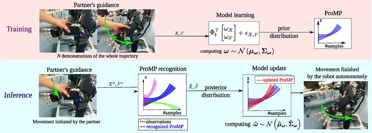
Figure 1. Conceptual use of the ProMP for predicting the desired trajectory to be performed by the robot in a collaborative task. Top: training phase, where ProMPs are learned from several human demonstrations. Bottom: inference phase (online), where from early observations, the robot recognizes the current (among the known) ProMP and predicts the human intention, i.e., the future evolution of the initiated trajectory.

In this article, we describe both the theoretical framework and the software that is used to perform this prediction. The software is currently implemented in Matlab and C++; it is open source, available on github:

https://github.com/inria-larsen/icubLearningTrajectories

and it has been tested both with a simulated iCub in Gazebo and the real iCub. In simulation, physical guidance is provided by the Geomagic Touch⁶; on the real robot, the human operator simply grabs the robot’s forearm.

We also provide a practical example of the software that realizes the exemplifying problems. In the example, the recorded trajectory is composed of both the Cartesian position and the forces at the end effector. Notably, in previous studies (Paraschos et al., 2015), ProMPs were used to learn movement primitives using joint positions. Here, we use Cartesian positions instead of joints positions to exploit the redundancy of the robotic arm in performing the desired task in the 3D space. At the control level of the iCub, this choice requires the iCub to control its lower-level (joint torque) movement with the Cartesian controller (Pattacini et al., 2010) instead of using the direct control at joint level. As for the forces, we rely on a model-based dynamics estimation that exploits the 6 axis force/torque sensors (Ivaldi et al., 2011; Fumagalli et al., 2012). All details for the experiments are presented in the article and the software tutorial.

To summarize, the contributions of this article are as follows:

• the description of a theoretical framework based on ProMPs for predicting the human desired trajectory and goal during physical human–robot interaction, providing the following features: recognition of the current task, estimation of the task duration, and prediction of the future trajectory;

• an experimental study about how multimodal information can be used to improve the estimation of the duration/speed of an initiated trajectory;

• the open-source software to realize an intention recognition application with the iCub robot, both in simulation and on the real robot.

The article is organized as follows. In Section 2, we review the literature about intentions in Human–Robot Interaction (HRI), probabilistic models for motion primitives, and their related software. In Section 3, we describe the theoretical tools that we use to formalize the problem of predicting the intention of the human during interaction. Particularly, we describe the ProMPs and their use for predicting the evolution of a trajectory given early observations. In Section 4, we overview the software organization and the interconnection between our software and the iCub’s main software, both for the real and simulated robot. The following sections are devoted to presenting our software and its use for predicting intention. We choose to present three examples of increasing complexity, with the simulated and real robot. We provide and explain in detail a software example for a 1-DOF trajectory in Section 5. In Sections 6 and 7, we present the intention recognition application with the simulated and real iCub, respectively. In the first examples with the robot, the “tasks” are exemplified by simple reaching movements, to provide simple and clear trajectories that help the reader understand the method, whereas the last experiment with the robot is a collaborative object sorting task. Section 8 provides the links to the videos showing how to use the software in simulation and on the iCub. Finally, in Section 10, we discuss our approach and its limitations and outline our future developments.

2. Related Work

In this article, we propose a method to recognize the intention of the human partner collaborating with the robot, formalized as the target and the “future” trajectory associated with a skill, modeled by a goal-directed Probabilistic Movement Primitive. In this section, we briefly overview the literature about intention recognition in human–robot interaction and motion primitives for learning of goal-directed robotic skills.

2.1. Intention during Human–Robot Interaction

When humans and robots collaborate, mutual understanding is paramount for the success of any shared task. Mutual understanding means that the human is aware of the robot’s current task, status, goal, available information, that he/she can reasonably predict or expect what it will do next, and vice versa. Recognizing the intention is only one piece of the problem but still plays a crucial part for providing anticipatory capabilities.

Formalizing intention can be a daunting task, as one may find it difficult to provide a unique representation that explains the intention for very low-level goal-directed tasks (e.g., reaching a target object and grasping it) and for very high-level, complex, abstract or cognitive tasks (e.g., change a light bulb on the ceiling—by building a stair composed of many parts, climbing it and reaching the light bulb on the ceiling, etc.). Demiris (2007) reviews different approaches of action recognition and intention prediction.

From the human’s point of view, understanding the robot’s intention means that the human should find intuitive and non-ambiguous every goal-directed robot movement or actions, and it should be clear what the robot is doing or going to do (Kim et al., 2017). Dragan and Srinivasa (2014) formalized the difference between predictability and legibility: a motion is legible if an observer can quickly infer its goal, while a motion is predictable when it matches the expectations of the observer given its goal.

The problem of generating legible motions for robots has been addressed in many recent works. For example, Dragan and Srinivasa (2014) use optimization techniques to generate movements that are predictable and legible. Huang et al. (2017) apply an Inverse Reinforcement Learning method on autonomous cars to select the robot movements that are maximally informative for the humans and that will facilitate their inference of the robot’s objectives.

From the robot’s point of view, understanding the human’s intention means that the robot should be able to decipher the ensemble of verbal and non-verbal cues that the human naturally generates with his/her behavior, to identify, for a current task and context, what is the human intention. The more information (e.g., measurable signals from the human and the environment) is used, the better and more complex the estimation can be.

The simplest form of intention recognition is to estimate the goal of the current action, under the implicit assumption that each action is a goal-directed movement.

Sciutti et al. (2013) showed that humans implicitly attribute intentions in form of goals to robot motions, proving that humans exhibit anticipatory gaze toward the intended goal. Gaze was also used by Ivaldi et al. (2014a) in a human–robot interaction game with iCub, where the robot (human) was tracking the human (robot) gaze to identify the target object. Ferrer and Sanfeliu (2014) proposed the Bayesian Human Motion Intentionality Prediction algorithm, to geometrically compute the most likely target of the human motion, using Expectation–Maximization and a simple Bayesian classifier. In Wang et al. (2012), a method called Intention-Driven Dynamics model, based on Gaussian Process Dynamical Models (GPDM) (Wang et al., 2005), is used to infer the intention of the robot’s partner during a ping-pong match, represented by the target of the ball, by analyzing the entire human movement before the human hits the ball. More generally, modeling and descriptive approaches can be used to match predefined labels with measured data (Csibra and Gergely, 2007).

A more complex form of intention recognition is to estimate the future trajectory from the past observations. In a sense, to estimate $\left[x_{t+1},\dots ,x_{t+T_{\mathit{\text{future}}}}\right]=f\left(x_t,x_{t-1},\dots ,x_{t-T_{\mathit{\text{past}}}}\right)$. This problem, very similar to the estimate of the forward dynamics model of a system, is frequently addressed by researchers in model predictive control, where being able to “play” the system evolving in time is the basis for computing appropriate robot controls. When a trajectory can be predicted by an observer from early observations of it, we can say that the trajectory is not only legible, but predictable. A systematic approach for predicting a trajectory is to reason in terms of movement primitives, in such a way that the sequence of points of the trajectory can be generated by a parametrized time model or a parametrized dynamical system. For example, Palinko et al. (2014) plan reaching trajectories for object carrying that are able to convey information about the weight of the transported object. More generally, in generative approaches (Buxton, 2003), latent variables are used to learn models for the primitives, both to generate and infer actions. The next subsection will provide more detail about the state-of-the-art techniques for generating movement primitives.

In Amor et al. (2014), the robot first learns Interaction Primitives by watching two humans performing an interactive task, using motion capture. The Interaction Primitive encapsulates the dependencies between the two human movements. Then, the robot uses the Interaction Primitive to adapt its behavior to its partner’s movement. Their method is based on Dynamics Motor Primitives (Ijspeert et al., 2013), where a distribution over the DMP’s parameters is learned. Notably, in this article, we did not follow the same approach to learn Interaction Primitives, since there is a physical interaction that makes the user’s and the robot’s movements as one joint movements. Moreover, there is no latency between the partner’s early movement and the robot’s, because the robot’s arm is physically driven by the human until the latter breaks the contact.

Indeed, most examples in the literature focus on kinematic trajectories, corresponding to gestures that are typically used in dyadic interactions characterized by a coordination of actions and reactions. Whenever the human and robot are also interacting physically, collaborating on a task with some exchange of forces, then the problem of intention recognition becomes more complex. Indeed, the kinematics information provided by the “trajectories” cannot be analyzed without taking into account the haptic exchange and the estimation of the “roles” of the partners in leading/following each other.

Estimating the current role of the human (master/slave or leader/follower) is crucial, as the role information is necessary to coherently adapt the robot’s compliance and impedance at the level of the exchanged contact forces. Most importantly, adapting the haptic interaction can be used by the robot to communicate when it has understood the human intent and is able to finish the task autonomously, mimicking the same type of implicit non-verbal communication that is typical of humans.

For example, in Gribovskaya et al. (2011), the robot infers the human intention utilizing the measure of the human’s forces and by using Gaussian Mixture Models. In Rozo Castañeda et al. (2013), the arm impedance is adapted by a Gaussian Mixture Model based on measured forces and visual information. Many studies focused on the robot’s ability to act only when and how its user wants (Carlson and Demiris, 2008; Soh and Demiris, 2015) and to not interfere with the partner’s forces (Jarrassé et al., 2008) or actions (Baraglia et al., 2016).

In this article, we describe our approach to the problem of recognizing the human intention during collaboration by providing an estimate of the future intended trajectory to be performed by the robot. In our experiments, the robot does not adapt its role during the physical interaction but simply switches from follower to leader when the human breaks contact with it.

2.2. Movement Primitives

Movement Primitives (MPs) are a well established paradigm for representing complex motor skills. The most known method for representing movement primitives is probably the Dynamic Movement Primitives (DMPs) (Schaal, 2006; Ijspeert et al., 2013; Meier and Schaal, 2016). DMPs use a stable non-linear attractor in combination with a forcing term to represent the movement. The forcing term enables to follow specific movement, while the attractor asserts asymptotic stability. In a recent paper, Meier and Schaal (2016) proposed an extension to DMPs, called PDMP (Probabilistic Dynamic Movement Primitive). This method improves DMP with probabilistic properties to measure the likelihood that the movement primitive is executed correctly and to perform inference on sensor measurement. However, the PDMPs do not have a data-driven generalization and can deviate arbitrarily from the demonstrations. This last difference can be critical for our applications with the humanoid robot iCub, since uncertainties are unavoidable and disturbances may happen frequently and destabilize the robot movement (for example, an unexpected collision during the movement). Thus, the ProMPs method is more accurate for our software.

Ewerton et al. (2015), Paraschos et al. (2013b), and Maeda et al. (2014) compared ProMPs and DMPs for learning primitives and specifically interaction primitives. With the DMP model, at the end of the movement, only a dynamic attractor is activated. Thus, it always reaches a stable goal. The properties allowed by both methods are temporal scaling of the movement, learning from a single demonstration, and generalizing to new final position. With ProMPs, we have in addition the ability to do inference (thanks to the distribution), to force the robot to pass by several initial via points (the early observations), to know the correlation between the input of the model, and to co-activate some ProMPs. In our study, we need these features, because the robot must determine a trajectory that passes by the early observations (beginning of the movement where the user guides physically the robot).

A Recurrent Neural Networks (RNN) approach (Billard and Mataric, 2001) used a hierarchy of neural networks to simulate the activation of areas in human brain. The network can be trained to infer the state of the robot at the next point in time, given the current state. The authors propose to train the RNN by minimizing the error between the inferred position of the next time step and the ground truth obtained from demonstrations.

Hidden Markov Models (HMMs) for movement skills were introduced by Fine et al. (1998). This method is often used to categorize movements, where a category represents a movement primitive. This method also allows to represent the temporal sequence of a movement. In Nguyen et al. (2005), they use learned Hierarchical Hidden Markov Model (HHMMs) to recognize human behaviors efficiently. In Ren and Xu (2002), they present the Primitive-based Coupled-HMM (CHMM) approach, for human natural complex action recognition. In this approach, each primitive is represented by a Gaussian Mixture Model.

Adapting Gaussian Mixture Models is another method used to learn physical interaction with learning. In Evrard et al. (2009), they use GMMs and Gaussian Mixture Regression to learn, in addition to the position (joint information), force information. Using this method, a humanoid robot is able to collaborate in one dimension with its partner for a lifting task. In this article, we will also use (Cartesian) position and force information to allow our robot to interact physically with its partner.

A subproblem of movement recognition is that robots need to estimate the duration of the trajectory to align a current trajectory with learned movements. In our case, at the beginning of the physical Human–Robot Interaction (pHRI), the robot observes a partial movement guided by its user. Given this partial movement, the robot must first estimate what the current state of the movement is to understand what its partner intent is. Thus, it needs to estimate the partial movement’s speed.

Fitts’ law models the movement duration for goal-directed movements. This model is based on the assumption that the movement duration is a linear function of the difficulty to achieve a target (Fitts, 1992). In Langolf et al. (1976), they show that by modifying the target’s width, the shape of the movement changes. Thus, it is difficult to apply Fitt’s law when the size of the target can change. In Langolf et al. (1976) and Soechting (1984), they confirm this idea by showing that the shape of the movement changes with the accuracy required by the goal position of the movement.

Dynamics Time Warping (DTW) is a method to find the correlation between two trajectories that have different durations, in a more robust way than the Euclidean distance. In Amor et al. (2014), they modify the DTW algorithm to match a partial movement with a reference movement. Many improvements over this method exist. In Keogh (2002), they propose a robust method to improve the indexation. The calculation speed of DTW is improved using different methods, such as FastDTW, Lucky Time Warping, or FTW. An explanation and comparison of these methods are presented in Silva and Batista (2016), where they add their own computation speed improvement by using a method called Pruned Warping Paths. This method allows the deletion of unlikely data. However, a drawback of this well-known DTW method is they do not preserve the global trajectory’s shape.

In Maeda et al. (2014), where they use a probabilistic learning of movement primitives, they improve the duration estimation of movements by using a different time warping method. This method is based on a Gaussian basis model to represent a time warping function and, instead of DTW, it forces a local alignment between the two movements without “jumping” some index. Thus, the resulting trajectories are more realistic, smoother, and this method preserves the global trajectories’ shapes.

For inferring the intention of the robot’s partner, we use Probabilistic Movement Primitives (ProMPs) (Paraschos et al., 2013a). Specifically, we use the ProMP’s conditioning operator to adapt the learned skills according to observations. The ProMPs can encode the correlations between forces and positions and allow better prediction of the partner’s intention. Further, the phase of the partner’s movement can be inferred, and therefore the robot can adapt to the partner’s velocity changes. ProMPs are more efficient for collaborative tasks, as shown in Maeda et al. (2014), where in comparison to DMPs, the root-mean square error of the predictions is lower.

2.3. Related Open-Source Software

One of the goals of this article is to introduce an open-source software for the iCub (but potentially for any other robot), where the ProMP method is used to recognize human intention during collaboration, so that the robot can execute initiated actions autonomously. This is not the first open-source implementation for representing movement primitives: however, it has a novel application and a rationale that makes it easy to use with the iCub robot.

In Table 1, we report on the main software libraries that one can use to learn movement primitives. Some have been also used to realize learning applications with iCub, e.g., Lober et al. (2014) and Stulp et al. (2013) or to recognize human intention. However, the software we propose here is different: it provides an implementation of ProMPs used explicitly for intention recognition and prediction of intended trajectories. It is interfaced with iCub, both real and simulated, and addresses in the specific case of physical interaction between the human and the robot. In short, it is a first step toward adding intention recognition ability to the iCub robot.

TABLE 1

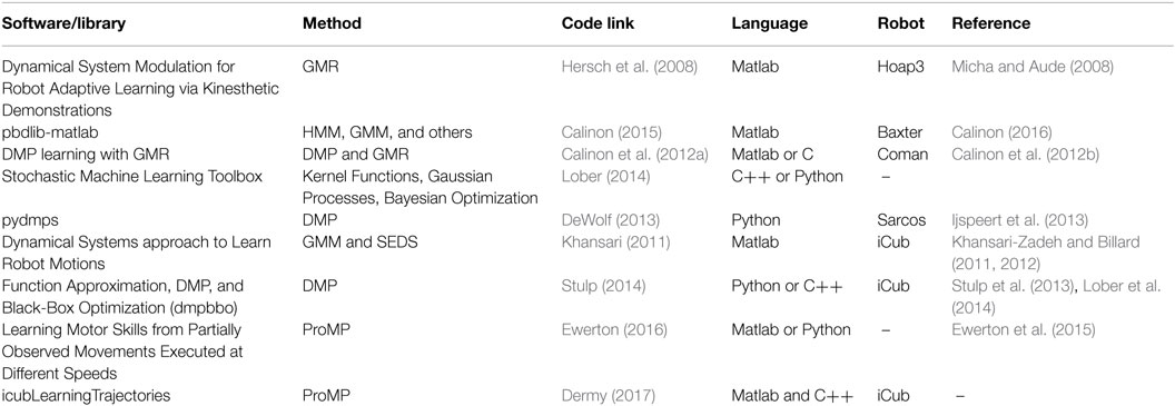
Table 1. Open-source software libraries implementing movement primitives and their application to different known robots.

3. Theoretical Framework

In this section, we present the theoretical framework that we use to tackle the problem of intent recognition: we describe the ProMPs and how they can be used to predict trajectories from early observations.

In Section 2, we formulate the problem of learning a primitive for a simple case, where the robot learns the distribution from several demonstrated trajectories. In Section 3.3, we formulate and provide the solution to the problem of predicting the “future” trajectory from early observations (i.e., the initial data points). In Section 3.4, we discuss the problem of predicting the time modulation, i.e., predicting the global duration of the predicted trajectory. This problem is non-trivial, as by construction the demonstrated trajectories are “normalized” in duration when the ProMP is learned.⁷ In Section 3.5, we explain how to recognize, from the early observations, to which of many known skills (modeled by ProMPs) the current trajectory belongs. In all these sections, we tried to present the theoretical aspects related to the use of ProMPs for the intention recognition application.

Practical examples of these theoretical problems are presented and explained later in sections 5–7. Section 5 explains how to use our software, introduced in Section 4, for learning one ProMP for a simple set of 1-DOF trajectories. Section 6 presents an example with the simulated iCub in Gazebo, while Section 7 presents an example with the real iCub.

3.1. Notation

To facilitate understanding of the theoretical framework, we first introduce the notations we use in this section and throughout the remainder of the article.

3.1.1. Trajectories

• $X\left(t\right)\in {ℛ}^3$, X(t) = [x(t), y(t), z(t)]^T: the x/y/z-axis Cartesian coordinate of the robot’s end effector.

• $F\left(t\right)\in {ℛ}^6$, F(t) = [f_x, f_y, f_z, m_x, m_y, m_z]^T: the wrench contact forces, i.e., the external forces and moments measured by the robot at the contact level (end effector).

• $\xi \left(t\right)\in {ℛ}^D$: the generic vector containing the current value or state of the trajectories at time t. It can be monodimensional (e.g., ξ(t) = [z(t)]), or multidimensional (e.g., ξ(t) = [X(t), F(t)]^T), depending on the type of trajectories that we want to represent with the ProMP.

• $\Xi ={\Xi }_{\left[1:t_f\right]}={\left[\xi \left(1\right),\dots ,\xi \left(t_f\right)\right]}^{\text{T}}\in {ℛ}^{D\cdot t_f}$ is an entire trajectory, consisting of t_f samples or data points.

• ${\Xi }_{i\left[1:t_{\mathit{\text{fi}}}\right]}$ is the i-th demonstration (trajectory) of a task, consisting of t_fi samples or data points.

3.1.2. Movement Primitives

• k ∈ [1 : K]: the k-th ProMP, among a set of K ProMPs that represent different tasks/actions.

• n_k: number of recorded trajectories for each ProMP.

• $S_k=\left\{{\Xi }_{\left\{k,1\right\}},\dots ,{\Xi }_{\left\{k,n_k\right\}}\right\}$: set of n_k trajectories for the k-th ProMP.

• $\xi \left(t\right)={\mathrm{\Phi }}_t\omega +{\epsilon }_{\xi }$ is the model of the trajectory with:

• ${\epsilon }_{\xi }\sim \mathcal{N}\left(0,\beta \right)$: expected trajectory noise.

• ${\mathrm{\Phi }}_t\in {ℛ}^{D\times D\cdot M}$: radial basis functions (RBFs) used to model trajectories. It is a block diagonal matrix.

– M: number of RBFs.

– ${\psi }_{\mathit{\text{ji}}}\left(t\right)=\frac{e^{\frac{-{\left(t-c_i\right)}^2}{2h}}}{{\sum }_{m=1}^M{e}^{\frac{-{\left(t-c_m\right)}^2}{2h}}}$: i-th RBF for all inputs j ∈ [1 : D].

It must be noted that the upper term comes from a Gaussian $\frac{1}{\sqrt{2\pi h}}{e}^{\frac{-{\left(t-c_i\right)}^2}{2h}}$, where c_i and h are, respectively, the center and variance of the i-th Gaussian. In our RBF formulation, we normalize all the Gaussians.

• $\omega \in {ℛ}^{D\cdot M}$: time-independent parameter vector weighting the RBFs, i.e., the parameters to be learned.

• $p\left(\omega \right)\sim \mathcal{N}\left({\mu }_{\omega },{\Sigma }_{\omega }\right)$: normal distribution computed from a set $\left\{\omega {}_1,\dots ,\omega {}_n\right\}$. It represents the distribution of the modeled trajectories, also called prior distribution.

3.1.3. Time Modulation

• $\overline{s}$: number of samples used as reference to rescale all the trajectories to the same duration.

• ${\mathrm{\Phi }}_{{\alpha }_{i}t}\in {ℛ}^{D\times D\cdot M}$: the RBFs rescaled to match the Ξ_i trajectory duration.

• ${\alpha }_i=\frac{\overline{s}}{t_{\mathit{\text{fi}}}}$: temporal modulation parameter of the i-th trajectory.

• $\alpha ={\mathrm{\Psi }}_{{\delta }_{n_o}}{\omega }_{\alpha }+{\epsilon }_{\alpha }$ is the model of the function mapping ${\delta }_{n_o}$ into the temporal modulation parameter α, with:

– Ψ: a set of RBFs used to model the mapping between ${\delta }_{n_o}$ and α;

– ${\delta }_{n_o}$ is the variation of the trajectory during the first n_o observations (data points); it can be ${\delta }_{n_o}=\xi \left(n_o\right)-\xi \left(1\right)$ if the entire trajectory variables (e.g., Cartesian position and forces) are considered, or more simply ${\delta }_{n_o}=X\left(n_o\right)-X\left(1\right)$ if only the variation in terms of Cartesian position is considered;

– ω_α: the parameter vector weighting the RBFs of the Ψ matrix.

3.1.4. Inference

• ${\Xi }^o={\left[X^o,F^o\right]}^{\text{T}}={\left[{\xi }^o\left(1\right),\dots ,{\xi }^o\left(n_o\right)\right]}^{\text{T}}$: early-trajectory observations, composed of n_o data points.

• ${\Sigma }_{\xi }^o$: noise of the initiated trajectory observation.

• $\widehat{\alpha }$: estimated time modulation parameter of a trajectory to infer.

• ${\widehat{t}}_f=\frac{\overline{s}}{\widehat{\alpha }}$: estimated duration of a trajectory to infer.

• ${\Xi }^{\ast }=\left[{\xi }^o\left(1\right),\dots ,{\xi }^o\left(n_o\right),{\xi }^{\ast }\left(n_o+1\right),\dots ,{\xi }^{\ast }\left(t_f\right)\right]$: ground truth of the trajectory for the robot to infer.

• $\widehat{\Xi }={\left[\widehat{X},\widehat{F}\right]}^{\text{T}}={\left[{\xi }^o\left(1\right),\dots ,{\xi }^o\left(n_o\right),\widehat{\xi }\left(n_o+1\right),\dots ,\widehat{\xi }\left({\widehat{t}}_f\right)\right]}^{\text{T}}$: the estimated trajectory.

• $p\left(\widehat{\omega }\right)\sim \mathcal{N}\left({\widehat{\mu }}_{\omega },{\widehat{\mathrm{\sigma }}}_{\omega }\right)$: posterior distribution of the parameter vector of a ProMP using the observation Ξ^o.

• $\widehat{k}$: index of the recognized ProMP from the set of K known (previously learned) ProMPs.

3.2. Learning a Probabilistic Movement Primitive (ProMP) from Demonstrations

Our toolbox to learn, replay and infer the continuation of trajectories is written in Matlab and available at:

https://github.com/inria-larsen/icubLearningTrajectories/tree/master/MatlabProgram

Let us assume the robot has recorded a set of n₁ trajectories: $\left\{{\Xi }_1,\dots ,{\Xi }_{n_1}\right\}$, where the i-th trajectory is ${\Xi }_i=\left\{\xi \left(1\right),\dots ,\xi \left(t_{f_i}\right)\right\}$. ξ(t) is the generic vector containing all the variables to be learned at time t, with the ProMP method. It can be monodimensional (e.g., ξ(t) = [z(t)] for the z-axis Cartesian coordinate), or multidimensional (e.g., ξ(t) = [X(t), F(t)]^T). Note that the duration of each recorded trajectory (i.e., $t_{f_i}$) may be variable. To find a common representation in terms of primitives, a time modulation is applied to all trajectories, such that they have the same number of samples $\overline{s}$ (see details in Section 3.4). Such modulated trajectories are then used to learn a ProMP.

A ProMP is a Bayesian parametric model of the demonstrated trajectories in the following form:

$\xi \left(t\right)={\mathrm{\Phi }}_t\omega +{\epsilon }_{\xi },$ (1)

where ω ∈ R^M is the time-independent parameter vector weighting the RBFs, ${\epsilon }_{\xi }\sim \mathcal{N}\left(0,\beta \right)$ is the trajectory noise, and Φ_t is a vector of M radial basis functions evaluated at time t:

${\mathrm{\Phi }}_t=\left[{\psi }_1\left(t\right),{\psi }_2\left(t\right),\dots .,{\psi }_M\left(t\right)\right]$

with

$\left\{\begin{array}{cc}{\psi }_i\left(t\right)\hfill & =\frac{1}{{\sum }_{j=1}^M{\psi }_j\left(t\right)}\mathit{\text{exp}}\left\{\frac{-{\left(t-c\left(i\right)\right)}^2}{2h}\right\}\hfill \\ c\left(i\right)\hfill & =i∕M\hfill \\ h\hfill & =1∕M^2.\hfill \end{array}\right.$ (2)

Note that all the ψ functions are scattered across time.

For each Ξ_i trajectory, we compute the ω_i parameter vector to have ${\xi }_i\left(t\right)={\mathrm{\Phi }}_t{\omega }_i+{\epsilon }_{\xi }$. This vector is computed to minimize the error between the observed ξ_i(t) trajectory and its model ${\mathrm{\Phi }}_t{\omega }_i+{\epsilon }_{\xi }$. This is done using the Least Mean Square algorithm, i.e.:

${\omega }_i={\left({\mathrm{\Phi }}_t^{\top }{\mathrm{\Phi }}_t\right)}^{-1}{\mathrm{\Phi }}_t^{\top }{\xi }_i\left(t\right).$ (3)

To avoid the common issue of the matrix ${\mathrm{\Phi }}_t^{\text{T}}{\mathrm{\Phi }}_t$ in equation (3) not being invertible, we add a diagonal term and perform Ridge Regression:

${\omega }_i={\left({\mathrm{\Phi }}_t^{\top }{\mathrm{\Phi }}_t+\mathrm{\lambda }\right)}^{-1}{\mathrm{\Phi }}_t^{\top }{\xi }_i\left(t\right),$ (4)

where $\mathrm{\lambda }={10}^{-11}\cdot 1_{D\cdot M\times D\cdot M}$ is a parameter that can be tuned by looking at the smallest singular value of the matrix ${\mathrm{\Phi }}_t^{\text{T}}{\mathrm{\Phi }}_t$.

Thus, we obtain a set of these parameters: $\left\{\omega {}_1,\dots ,\omega {}_n\right\}$, upon which a distribution is computed. Since we assume Normal distributions, we have:

$\begin{array}{ll}\hfill p\left(\omega \right)& \sim \mathcal{N}\left({\mu }_{\omega },{\Sigma }_{\omega }\right)\end{array}$ (5)

$\begin{array}{l}\hfill \mathrm{with}{\mu }_{\omega }=\frac{1}{n}{\displaystyle \sum _{i=1}^n{\omega }_i}\end{array}$ (6)

$\begin{array}{ll}\hfill \mathrm{and}{\Sigma }_{\omega }& =\frac{1}{n-1}{\displaystyle \sum _{i=1}^n}{\left({\omega }_i-{\mu }_{\omega }\right)}^{\top }\left({\omega }_i-{\mu }_{\omega }\right).\end{array}$ (7)

The ProMP captures the distribution over the observed trajectories. To represent this movement primitive, we usually use the movement that passes by the mean of the distribution. Figure 2 shows the ProMP for a 1-DOF lifting motion, with a number of reference samples $\overline{s}$ = 100 and number of basis functions M = 5.

FIGURE 2

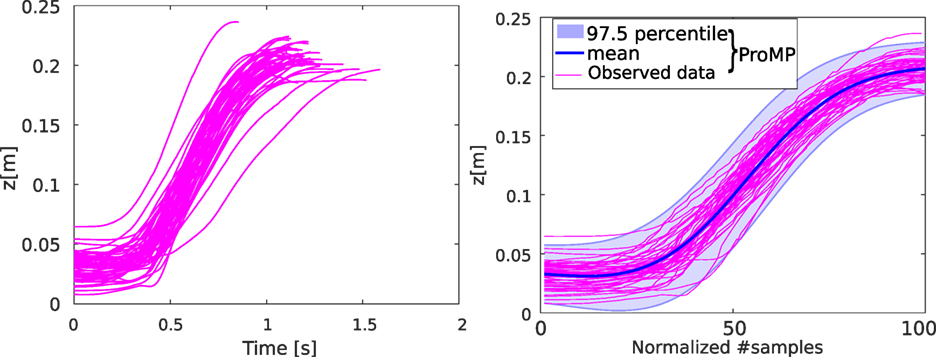
Figure 2. The observed trajectories are represented in magenta. The corresponding ProMP is represented in blue. The following parameters are used: $\overline{\mathit{\text{s}}}=\text{100}$ for the reference number of samples, M = 5 for the number of RBFs spread over time, and h = 0.04 $\left(=\frac{\text{1}}{{\mathit{\text{M}}}^{\text{2}}}\right)$ the variance of the RBFs.

This example is included in our Matlab toolbox as demo_plot1DOF.m. The explanation of this Matlab script is presented in Section 5. More complex examples are also included in the scripts demo_plot*.m.

3.3. Predicting the Future Movement from Initial Observations

Once the ProMP $p\left(\omega \right)\sim \mathcal{N}\left({\mu }_{\omega },{\Sigma }_{\omega }\right)$ of a certain task has been learned,⁸ we can use it to predict the evolution of an initiated movement. An underlying hypothesis is that the observed movement follows to this learned distribution.

Suppose that the robot measures the first n_o observations of the trajectory to predict (e.g., lifting the arm). We call these observations Ξ^o = [ξ^o(1), …, ξ^o(n_o)]. The goal is then to predict the evolution of the trajectory after these n_o observations, i.e., find $\left\{\widehat{\xi }\left(n_o+1\right),\dots ,\widehat{\xi }\left({\widehat{t}}_f\right)\right\}$, where ${\widehat{t}}_f$ is the estimation of the trajectory duration (see Section 3.4). This is equivalent to predicting the entire $\widehat{\Xi }$ trajectory where the first n_o samples are known and equal to the observations: $\widehat{\Xi }=\left\{{\xi }^o\left(1\right),\dots ,{\xi }^o\left(n_o\right),\widehat{\xi }\left(n_o+1\right),\dots ,\widehat{\xi }\left(t_{{\widehat{t}}_f}\right)\right\}$. Therefore, our prediction problem consists of predicting $\widehat{\Xi }$ given the Ξ^o observations.

To do this prediction, we start from the learned prior distribution p(ω), and we find the $\widehat{\omega }$ parameter within this distribution that generates $\widehat{\Xi }$. To find this $\widehat{\omega }$ parameter, we update the learned distribution $p\left(\widehat{\omega }\right)\sim \mathcal{N}\left({\widehat{\mu }}_{\omega },{\widehat{\Sigma }}_{\omega }\right)$ using the following formulae:

$\left\{\begin{array}{c}{\widehat{\mu }}_{\omega }={\mu }_{\omega }+K\left({\Xi }^o-{\mathrm{\Phi }}_{\left[1:n_o\right]}{\mu }_{\omega }\right)\hfill \\ {\widehat{\Sigma }}_{\omega }={\Sigma }_{\omega }-K\left({\mathrm{\Phi }}_{\left[1:n_o\right]}{\Sigma }_{\omega }\right),\hfill \end{array}\right.$ (8)

where K is a gain computed by the following equation:

$K={\Sigma }_{\omega }{\mathrm{\Phi }}_{\left[1:n_o\right]}^{\top }{\left({\Sigma }_{\xi }^o+{\mathrm{\Phi }}_{\left[1:n_o\right]}{\Sigma }_{\omega }{\mathrm{\Phi }}_{\left[1:n_o\right]}^{\top }\right)}^{-1}.$ (9)

Equations (8) and (9) can be computed through the marginal and conditional distributions (Bishop, 2006; Paraschos et al., 2013a), as detailed in Appendix A.

Figure 3 shows the predicted trajectory for the lifting motion of the left arm of iCub. The different graphs show inferred trajectories when the robot observed n_o = 10, 30, 50, and 80% of the total trajectory duration. This example is also available in the toolbox as demo_plot1DOF.m. The nbData variable changes the percentage of known data. Thus, it will be visible how the inference improves according to this variable. An example of predicted trajectories of the arm lifting in Gazebo can be found in a provided video (see Section 8).

FIGURE 3

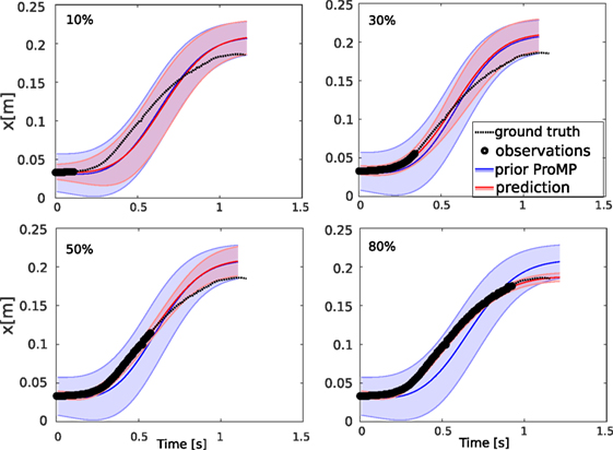
Figure 3. The prediction of the future trajectory given early observations, exploiting the information of the learned ProMP (Figure 2). The plots show the predicted trajectories after 10, 30, 50, and 80% of observed data points.

3.4. Predicting the Trajectory Time Modulation

In the previous section, we presented the general formulation of ProMPs, which makes the implicit assumption that all the observed trajectories have the same duration and thus the same sampling.⁹ That is why the duration of the trajectories generated by the RBF is fixed and equal to $\overline{s}$. Of course, this is valid only for synthetic data and not for real data.

To be able to address real experimental conditions, we now consider the variation of the duration of the demonstrated trajectories. To this end, we introduce a time modulation parameter α that maps the actual trajectory duration t_f to $\overline{s}$: $\alpha =\overline{s}∕t_f$. The normalized duration $\overline{s}$ can be chosen arbitrarily; for example it can be set to the average of the duration of the trajectories, e.g., $\overline{s}=\mathit{\text{mean}}\left(t_{f1},\dots ,t_{\mathit{\text{fK}}}\right)$. Notably, in the literature sometimes α is called phase (Paraschos et al., 2013a,b). The effect of α is to change the phase of the RBFs, which are scaled in time.

The time modulation of the i-th trajectory Ξ_i is computed by ${\alpha }_i=\frac{\overline{s}}{t_{\mathit{\text{fi}}}}$. Thus, we have $\alpha \cdot t\in \left[1:\overline{s}\right]$. Thus, the improved ProMP model is as follows:

${\xi }_t={\mathrm{\Phi }}_{\alpha t}\omega +{\epsilon }_t,$ (10)

where Φ_αt is the RBFs matrix evaluated at time αt. All the M Gaussian functions of the RBFs are spread over the same number of samples $\overline{s}$. Thus, we have the following:

${\mathrm{\Phi }}_{\alpha t}=\left[{\psi }_1\left(\alpha t\right),{\psi }_2\left(\alpha t\right),\dots .,{\psi }_M\left(\alpha t\right)\right].$

During the learning step, we record a set of α parameters: S_α = {α₁, …, α_n}. Then, using this set, we can replay the learned ProMP with different speeds. By default (e.g., when α = 1), the speed allows to finish the movement in $\overline{s}$ samples.

During the inference, the time modulation α of the partially observed trajectory is not known. Unless fixed a priori, the robot must estimate it. This estimation is critical to ensure a good recognition, as shown in Figure 4: the inferred trajectory (represented by the mean of the posterior distribution in red) does not have the same duration as the “real” intended trajectory (which is the ground truth). This difference is due to the estimation error of the time modulation parameter. This estimation $\widehat{\alpha }$ by default is computed as the mean of all the α_k observed during the learning:

$\widehat{\alpha }=\frac{\sum {\alpha }_k}{n_k}.$ (11)

FIGURE 4

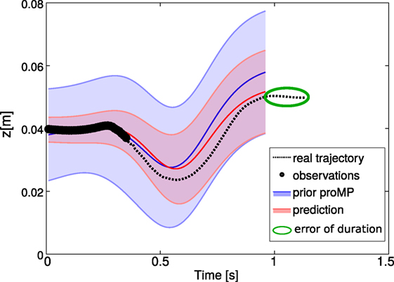
Figure 4. This plot shows the predicted trajectory given early observations (data points, in black), compared to the ground truth (e.g., the trajectory that the human intends to execute with the robot). We show the prior distribution (in light blue) and the posterior distribution (in red), which is computed by conditioning the distribution to match the observations. Here, the posterior simply uses the average α computed over the α₁, …, α_K of the K demonstrations. Without predicting the time modulation from the observations and using the average α, the predicted trajectory has a duration that is visibly different from the ground truth.

However, using the mean value for the time modulation is an appropriate choice only when the primitive represents goal-directed motions that are very regular, or for which we can reasonably assume that differences in the duration can be neglected (which is not a general case). In many applications, this estimation may be too rough.

Thus, we have to find a way to estimate the duration of the observed trajectory, which corresponds to accurately estimating the time modulation parameter $\widehat{\alpha }$. To estimate $\widehat{\alpha }$, we implemented four different methods. The first is the mean of all the α_k, as in equation (11). The second is the maximum likelihood, with

$\widehat{\alpha }={\mathrm{argmax}}_{\alpha \in S_{\alpha k}}\left\{\mathrm{loglikelihood}\left({\Xi }^o,{\mu }_{\omega {}_k},{\mathrm{\sigma }}_{\omega {}_k},{\alpha }_k\right)\right\}.$ (12)

The third is the minimum distance criterion, where we seek the best $\widehat{\alpha }$ that minimizes the difference between the observed trajectory ${\Xi }_t^o$ and the predicted trajectory for the first n_o data points:

$\widehat{\alpha }={\mathrm{argmin}}_{\alpha \in S_{\alpha k}}\left\{{\displaystyle \sum _{t=1}^{n_o}}\left|{\Xi }_t^o-{\mathrm{\Phi }}_{\alpha t}{\mu }_{\omega {}_k}\right|\right\}.$ (13)

The fourth method is based on a model: we assume that there is a correlation between α and the variation of the trajectory ${\delta }_{n_o}$ from the beginning until the time n_o. This “variation” ${\delta }_{n_o}$ can be computed as the variation of the position, e.g., ${\delta }_{n_o}=X\left(n_o\right)-X\left(1\right)$, or the variation in the entire trajectory, ${\delta }_{n_o}=\Xi \left(n_o\right)-\Xi \left(1\right)$, or any other measure of progress, if this hypothesis is appropriate for the type of task trajectories of the application.¹⁰ Indeed, the α can be linked also to the movement speed, which can be roughly approximated by $Ẋ=\frac{\delta X}{t_f}$ $\left(\dot{\Xi }=\frac{\delta \Xi }{t_f}\right)$. We model the mapping between ${\delta }_{n_o}$ and α by the following equation:

$\alpha =\mathrm{\Psi }{\left({\delta }_{n_o}\right)}^{\top }{\omega }_{\alpha }+{\epsilon }_{\alpha },$ (14)

where Ψ are RBFs, and ${\epsilon }_{\alpha }$ is a zero-mean Gaussian noise. During learning, we compute the ω_α parameter, using the same method as in equation (3). During the inference, we compute $\widehat{\alpha }=\mathrm{\Psi }{\left({\delta }_{n_o}\right)}^{\text{T}}{\omega }_{\alpha }$.

A comparison of the four methods for estimating α on a test study with iCub in simulation is presented in Section 6.6.

There exist other methods in the literature for computing α. For example, Ewerton et al. (2015) propose a method that models local variability in the speed of execution. In Maeda et al. (2016), they use a method that improves Dynamic Time Warping by imposing a smooth function on the time alignment mapping using local optimization. These methods will be implemented in the future works.

3.5. Recognizing One among Many Movement Primitives

Robots should not learn only one skills but many: different skills for different tasks. In our framework, tasks are represented by movement primitives, precisely ProMP. So it is important for the robot to be able to learn K different ProMPs and then be able to recognize from the early observations of a trajectory which of the K ProMPs the observations belong to.

During the learning step of a movement primitive k ∈ [1 : K], the robot observes different trajectories S_k = {Ξ₁, …, Ξ_n}. For each ProMP, it learns the distribution over the parameters vector $p\left(\omega \right)\sim \mathcal{N}\left({\mu }_{{\omega }_k},{\Sigma }_{{\omega }_k}\right)$, using equation (3). Moreover, the robot records the different phases of all the observed trajectories: S_αk = {α_1k, …, α_nk}.

After having learned these K ProMPs, the robot can use this information to autonomously execute a task trajectory. Since we are targeting collaborative movements, performed together with a partner at least at the beginning, we want the robot to be able to recognize from the first observations of a collaborative trajectory which is the current task that the partner is doing and what is the intention of the partner. Finally, we want the robot to be able to complete the task on its own, once it has recognized the task and predicted the future trajectory.

Let ${\Xi }^o={\left[{\Xi }_1\dots {\Xi }_{n_o}\right]}^{\text{T}}$ be the early observations of an initiated trajectory.

From these partial observations, the robot can recognize the “correct” (i.e., most likely) ProMP $\widehat{k}\in \left[1:K\right]$. First, for each ProMP k ∈ [1 : K], it computes the most likely phase (time modulation factor) ${\widehat{\alpha }}_k$ (as explained in Section 3.4), to obtain the set of ProMPs with the most likely duration: $S_{\left[{\mu }_{{\omega }_k},{\widehat{\alpha }}_k\right]}=\left\{\left({\mu }_{{\omega }_1},{\widehat{\alpha }}_1\right),\dots ,\left({\mu }_{{\omega }_K},{\widehat{\alpha }}_K\right)\right\}$.

Then we compute the most likely ProMP $\widehat{k}$ in $S_{\left[{\mu }_{{\omega }_k},{\widehat{\alpha }}_k\right]}$ according to some criterion. One possible way is to minimize the distance between the early observations and the mean of the ProMP for the first portion of the trajectory:

$\widehat{k}=\arg \underset{k\in [1:K]}{\min }\left[\frac{1}{n_o}{\displaystyle \mathrm{\sum }_{t=1}^{n_o}}\mathrm{|}{\Xi }_t-{\mathrm{\Phi }}_{{\widehat{\alpha }}_{k}t}{\mu }_{\omega {}_k}\mathrm{|}\right].$ (15)

In equation (15), for each ProMP k ∈ [1 : K], we compute the average distance between the observed early-trajectory Ξ_t and the mean trajectory of the ProMP ${\mathrm{\Phi }}_{{\widehat{\alpha }}_{k}t}{\mu }_{{\omega }_k}$, with t = [1 : n_o]. The most likely ProMP $\widehat{k}$ is selected by computing the minimum distance (arg min). Other possible methods for estimating the most likely ProMPs could be inspired by those presented in the previous section for estimating the time modulation, i.e., maximum likelihood or learned models.

Once identified the $\widehat{k}$-th most likely ProMP, we update its posterior distribution to take into account the initial portion of the observed trajectory, using equation (8):

$\left\{\begin{array}{cc}{\widehat{\mu }}_{\omega {}_{\widehat{k}}}\hfill & ={\mu }_{\omega {}_{\widehat{k}}}+K\left({\Xi }^o-{\mathrm{\Phi }}_{{\widehat{\alpha }}_{\widehat{k}}\left[1:n_o\right]}{\mu }_{\omega {}_{\widehat{k}}}\right)\hfill \\ {\widehat{\Sigma }}_{\omega {}_{\widehat{k}}}\hfill & ={\Sigma }_{\omega {}_{\widehat{k}}}-K\left({\mathrm{\Phi }}_{{\widehat{\alpha }}_{\widehat{k}}\left[1:n_o\right]}{\Sigma }_{\omega {}_{\widehat{k}}}\right)\hfill \\ K\hfill & ={\Sigma }_{\omega {}_{\widehat{k}}}{\mathrm{\Phi }}_{{\widehat{\alpha }}_{\widehat{k}}\left[1:n_o\right]}^{\top }{\left({\Sigma }_{{\xi }^o}+{\mathrm{\Phi }}_{{\widehat{\alpha }}_{\widehat{k}}\left[1:n_o\right]}{\Sigma }_{\omega {}_{\widehat{k}}}{\mathrm{\Phi }}_{{\widehat{\alpha }}_{\widehat{k}}\left[1:n_o\right]}^{\top }\right)}^{-1}\hfill \end{array}\right.$ (16)

with ${\widehat{\alpha }}_{\widehat{k}}\left[1:n_o\right]={\widehat{\alpha }}_{\widehat{k}}t$ (in matrix form), with t ∈ [1 : n_o].

Finally, the inferred trajectory is given by the following equation:

$\forall t\in \left[1:{\widehat{t}}_f\right],\widehat{\xi }\left(t\right)={\mathrm{\Phi }}_t{\widehat{\mu }}_{{\omega }_{\widehat{k}}}$

with the expected duration of the trajectory ${\widehat{t}}_f={\widehat{\alpha }}_k\overline{s}$. The robot is now able to finish the movement executing the most likely “future” trajectory $\widehat{\Xi }={\left[{\widehat{\xi }}_{n_o+1}\dots {\widehat{\xi }}_{t_f}\right]}^{\text{T}}$.

4. Software Overview

In this section, we introduce our open-source software with an overview of its architecture. This software is composed of two main modules, represented in Figure 5.

FIGURE 5

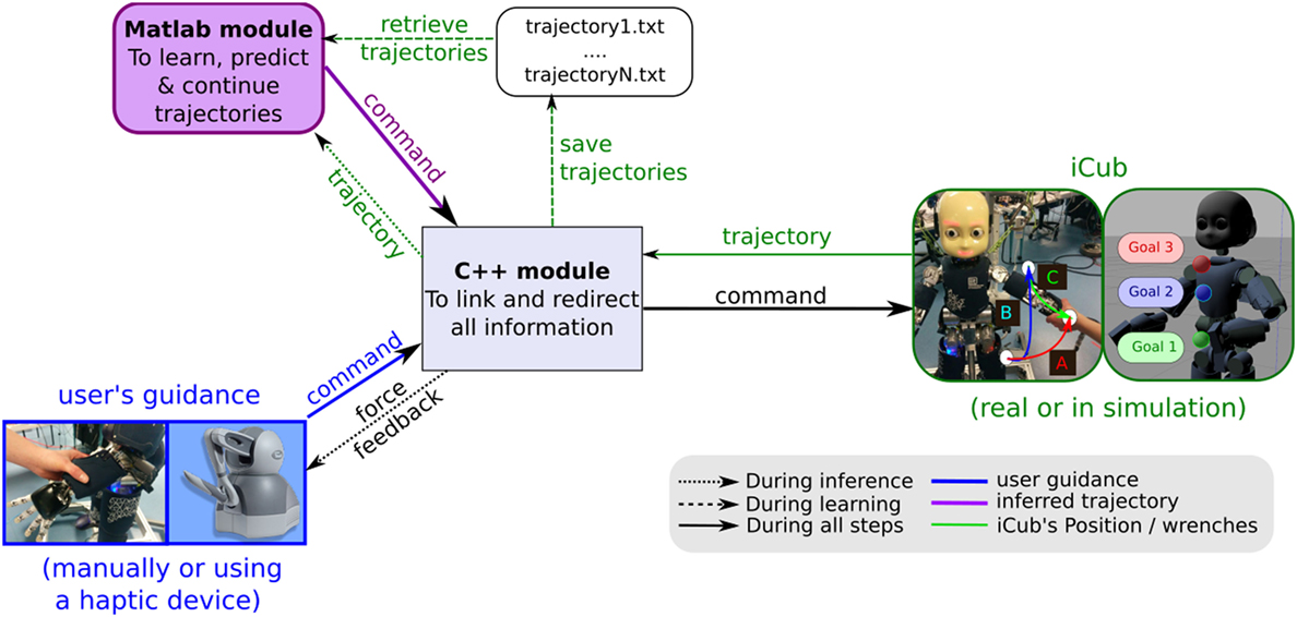
Figure 5. Software architecture and data flows. The robot’s control is done either by the user’s guidance (manually or through a haptic device) represented in blue, or by the Matlab module, in purple. The C++ module handles the control source to command the robot, as represented in black. Moreover, this module forwards information that comes from the iCub.

While the robot is learning the Probabilistic Movement Primitives (ProMPs) associated with the different tasks, the robot is controlled by its user. The user’s guidance can be either manual for the real iCub, or through a haptic device for the simulated robot.

A Matlab module allows replaying movement primitives or finishing a movement that has been initiated by its user. By using this module, the robot can learn distributions over trajectories, replay movement primitives (using the mean of the distribution), recognize the ProMP that best matches a current trajectory, and infer the future evolution (until the end target) of this trajectory.

A C++ module forwards to the robot the control that comes either from the user or from the Matlab module. Then, the robot is able to finish a movement initiated by its user (directly or through a haptic device) in an autonomous way, as shown in Figure 1.

We present the C++ module in Section 6.2 and the theoretical explanation of the Matlab module algorithms in Section 3. A guide to run this last module is first presented in Section 5 for a simple example, and in Section 6 for our application, where a simulated robot learns many measured information of the movements. Finally, we present results on the real iCub application in Section 7.

Our software is available through the GPL license, and publicly available at:

https://github.com/inria-larsen/icubLearningTrajectories.

Tutorial, readme, and videos can be found in that repository. First, the readme file describes how to launch simple demonstrations of the software. Videos present these demonstrations to simplify the understanding. In the next sections, we detail the operation of the demo program for a first case of 1-DOF primitive, followed by the presentation of the specific applications on the iCub (first simulated and then real).

5. Software Example: Learning a 1-DOF Primitive

In this section, we present the use of the software to learn ProMPs in a simple case of 1-DOF primitive. This example only uses the MatlabProgram folder, composed of:

• A sub-folder called “Data,” where there are trajectory sets used to learn movement primitives. These trajectories are stored in text files with the following information:

– input parameters: # input₁ # input₂ […]

– input parameters with time step: # timeStep # input₁ # input₂ […]

– recordTrajectories.cpp program recording: See Section 6.3 for more information.

• A sub-folder called “used_functions.” It contains all the functions used to retrieve trajectories, compute ProMPs, infer trajectories, and plot results. Normally, using this toolbox does not require understanding these functions. The first lines of these functions give an explanation of their functioning and precise what are the input(s) and output(s) parameters.

• Matlab scripts called “demo_*.m.” They are simple examples of how to use this toolbox.

The script demo_plot1DOF.m, can be used to compute a ProMP and to continue an initiated movement. The ProMP is computed from a dataset stored in a “.mat” file, called traj1_1DOF.mat. In this script, variables are first defined to make the script specific to the current dataset:

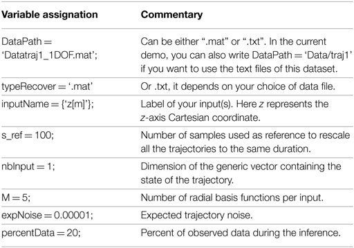
The variables include the following:

• DataPath is the path to the recorded data. If the data are stored in text files, this variable contains the folder name where text files are stored. These text files are called “recordX.txt,” with X ∈ [0: n − 1] if there are n trajectories. One folder is used to learn one ProMP. If the data are already loaded from a “.mat” file, write the whole path with the extension. The data in “.mat” match with the output of the Matlab function loadTrajectory.

• nbInput = D is the dimension of the input vector ξ_t.

• expNoise $={\Sigma }_{\xi }^o$ is the expected noise of the initiated trajectory. The smaller this variable is, the stronger the modification of the ProMP distribution will be, given new observations.

We will now explain more in detail the script. To recover data recorded in a “.txt” file, we call the function:

t{1} = loadTrajectory(PATH, nameT, varargin)

Its input parameters specify the path of the recorded data, the label of the trajectory. Other information can be added by using the varargin variable (for more detail, check the header of the function with the help comments). The output is an object that contains all the information about the demonstrated trajectories. It is composed of nbTraj, the number of trajectory; realTime, the simulation time; and y (and yMat), the vector (and matrix) trajectory set. Thus, t{1}.y{i} contains the i-th trajectory.

The Matlab function drawRecoverData(t{1}, inputName,’namFig’, nFig, varargin) plots in a Matlab figure (numbered nFig) the dataset of loaded trajectories. An example is shown in Figure 2, on the left. Incidentally, the different duration of the trajectories is visible: on average, it is 1.17 ± 0.42 s.

To split the entire dataset of demonstrated trajectories t{1} into a training dataset (used for learning the ProMPs) and a test dataset (used for the inference), call the function

[train, test] = partitionTrajectory(t{1}, partitionType, percentData, s_ref)

where if partitionType = 1, only one trajectory is in the test set and the others are placed in the training set, and if partitionType > 1 it corresponds to the percentage of trajectories that will be included in the training set.

The ProMP can be computed from the training set by using the function:

promp = computeDistribution(train, M, s_ref, c, h)

The output variable promp is an object that contains all the ProMP information. The first three input parameters have been presented before: train is the training set, M is the number of RBFs, and s_ref is the number of samples used to rescale all the trajectories. The last two input parameters c and h shape the RBFs of the ProMP model: c ∈ ${ℛ}^M$ is the center of the Gaussians and h ∈ ℛ their variance.

To visualize this ProMP, as shown in Figure 2, call the function:

drawDistribution(promp, inputName, s_ref)

For debugging purposes and to understand how to tune the ProMPs’ parameters, it is interesting to plot the overlay of the basis functions in time. Choosing an appropriate number of basis functions is important, as too few may be insufficient to approximate the trajectories under consideration, and too many could result in overfitting problems. To plot the basis functions, simply call:

drawBasisFunction(promp.PHI, M)

where promp.PHI is a set of RBFs evaluated in the normalized time range $t\in \left[1:\overline{s}\right]$.

Figure S1 in Supplementary Material shows at the top the basis functions before normalization, and at the bottom the ProMP modeled from these basis functions. From left to right, we change the number of basis functions. When there are not enough basis functions (left), the model is not able to correctly represent the shape of the trajectories. In the middle, the trajectories are well represented by the five basis functions. With more basis functions (right), the variance of the distribution decreases because the model is more accurate. However, arbitrarily increasing the number of basis functions is not a good idea, as it may not improve the accuracy of the model and worse it may cause overfitting.

Once the ProMP is learned, the robot can reproduce the movement primitive using the mean of the distribution. Moreover, it can now recognize a movement that has been initiated in this distribution and predict how to finish it. To do so, given the early n_o observations of a movement, the robot updates the prior distribution to match the early observed data points: through conditioning, it finds the posterior distribution, which can be used by the robot to execute the movement on its own.

The first step in predicting the evolution of the trajectory is to infer the duration of this trajectory, which is encoded by the time modulation parameter $\widehat{\alpha }$. The computation of this inference, which was detailed in Section 3.4, can be done by using the function:

[expAlpha, type, x] = inferenceAlpha(promp, test{1}, M, s_ref, c, h, test{1}.nbData, … expNoise, typeReco)

where typeReco is the type of criteria used to find the expected time modulation (“MO,” “DI,” or “ML” for model, distance or maximum likelihood methods); expAlpha = $\widehat{\alpha }$ is the expected time modulation; type is the index of the ProMP from which expAlpha has been computed, which we note in this article as k. To predict the evolution of the trajectory, we use equation (8) from Section 3.3. In Matlab, this is done by the function:

infTraj = inference(promp, test{1}, M, s_ref, c, h,… test{1}.nbData, expNoise, expAlpha).

where test{1}.nbData has been computed during the partitionTrajectory step. This variable is the number of observations n_o, representing the percentage of observed data (percentData) of the test trajectory (i.e., to be inferred) that the robot observes. infTraj = $\widehat{\Xi }$ is the inferred trajectory. Finally, to draw the inferred trajectory, we can call the function drawInference(promp, inputName, infTraj, test1, s_ref).

It can be interesting to plot the quality of the predicted trajectories as a function of the number of observations, as done in Figure 3.

Note that when we have observed a larger portion of the trajectory, the prediction of the remaining portion is more accurate.

Now we want to measure the quality of the prediction. Let ${\Xi }^{\ast }=\left[{\xi }^o\left(1\right),\dots ,{\xi }^o\left(n_o\right),{\xi }^{\ast }\left(n_o+1\right),\dots ,{\xi }^{\ast }\left(t_f^{\ast }\right)\right]$ be the real trajectory expected by the user. To measure the quality of the prediction, we can use:

• The likelihood of having the Ξ^* trajectory given the updated distribution p($\widehat{\omega }$).

• The distance between the Ξ^* trajectory and the $\widehat{\Xi }$ inferred trajectory.

However, according to the type of recognition typeReco used to estimate the time modulation parameter α from the early observations, a visible mismatch between the predicted trajectory and the real one can be visible even when a lot of observations are used. This is due to the error of the expectation of this time modulation parameter. In Section 3.4, we present the different methods used to predict the trajectory duration. These methods select the most likely $\widehat{\alpha }$ according to different criteria: distance; maximum likelihood; model of the α variable¹¹; and average of the observed α during learning.

Figure 6 shows the different trajectories predicted after n_o = 40% of the length of the desired trajectory is observed, according to the method used to estimate the time modulation parameter.

FIGURE 6

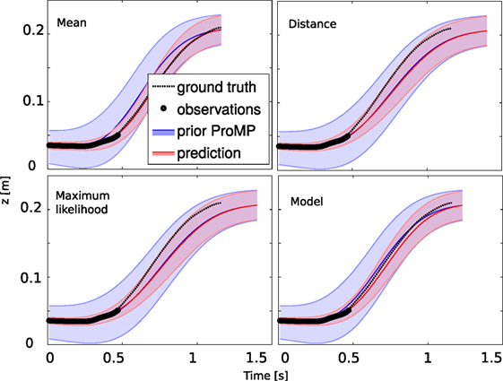
Figure 6. The prediction of the future trajectory given n_o = 40% of early observations from the learned ProMP computed for the test dataset (Figure 2). The plots show the predicted trajectory, using different criteria to estimate the best phases of the trajectory: using the average time modulation (equation (11)); using the distance criteria (equation (13)); using the maximum log-likelihood (equation (12)); or using a model of time modulation according to the time variation (equation (14)).

On this simple test, where the variation time is little as shown in Table 2, the best result is accomplished by the average of time modulation parameter of the trajectories used during the learning step. In more complicated cases, when the time modulation varies, the other methods will be preferable as seen in Section 3.5.

TABLE 2

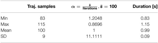
Table 2. Information about trajectories’ duration.

6. Application on the Simulated iCub: Learning Three Primitives

In this application, the robot learns multiple ProMPs and is able to predict the future trajectory of a movement initiated by the user, assuming the movement belongs to one of the learned primitives. Based on this prediction, it can also complete the movement once it has recognized the appropriate ProMP.

We simplify the three actions/tasks by reaching three different targets, represented by three colored balls in the reachable workspace of the iCub. The example is performed with the simulated iCub in Gazebo. Figure 7 shows the three targets, placed at different heights in front of the robot.

FIGURE 7

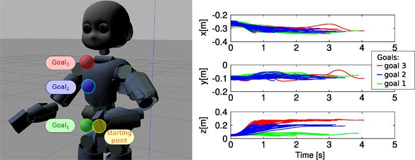
Figure 7. Left: the three colored targets that the robot must reach from the starting point; the corresponding trajectories are used to learn three primitives representing three skills. Right: the Cartesian position information of the demonstrated trajectories for the three reaching tasks.

In Section 6.1, we formulate the intention recognition problem for the iCub: the problem is to learn the ProMP from trajectories consisting of Cartesian positions in 3D¹² and the 6D wrench information measured by the robot during the movement. In Section 6.2, we describe the simulated setup of iCub in Gazebo, then in Section 6.3, we explain how trajectories are recorded, including force information, when we use the simulated robot.

6.1. Predicting Intended Trajectories by Using ProMPs

The model is based on Section 3, but here we want to learn more information during movements. We record this information in a multivariate parameter vector:

$\forall t,{\xi }_t=\left[\begin{array}{c}\hfill X_t\hfill \\ \hfill F_t\hfill \end{array}\right]\in {ℛ}^9,$

where $X_t\in {ℛ}^3$ is the Cartesian position of the robot’s end effector and $F_t\in {ℛ}^6$ the external forces and moments. In particular, F_t contains the user’s contact forces and moments. Let us call dim(ξ_t) = D, the dimension of this parameter vector.

The corresponding ProMP model is as follows:

${\xi }_t=\left[\begin{array}{c}\hfill X_t\hfill \\ \hfill F_t\hfill \end{array}\right]={\mathrm{\Phi }}_{\alpha t}\omega +{\epsilon }_t,$

where $\omega \in {ℛ}^{D\cdot M}$ is the time-independent parameter vector, ${\epsilon }_t=\left[\begin{array}{c}\hfill {\epsilon }_{X_t}\hfill \\ \hfill {\epsilon }_{F_t}\hfill \end{array}\right]\in {ℛ}^D$ is the zero-mean Gaussian i.i.d. observation noise, and ${\mathrm{\Phi }}_{\alpha t}\in {ℛ}^{D\times D\cdot M}$ a matrix of Radial Basis Functions (RBFs) evaluated at time αt.

Since we are in the multidimensional case, this Φ_αt block diagonal matrix is defined as follows:

${\mathrm{\Phi }}_{\alpha t}=\mathit{\text{BlockdiagonalMatrix}}\left({\varphi }_1,\dots ,{\varphi }_D\right)\in R^{D\times D\cdot M}\text{.}$

It is a diagonal matrix of D Radial Basis Functions (RBFs), where each RBF represents one dimension of the ξ_t vector and it is composed of M Gaussians, spread over same number of samples $\overline{s}$.

6.1.1. Learning Motion Primitives

During the learning step of each movement primitive k ∈ [1 : 3], the robot observes different trajectories S_k = {Ξ₁, …, Ξ_n}_k, as presented in Section 6.3.

For each trajectory ${\Xi }_{i\left[1:t_{\mathit{\text{fi}}}\right]}={\left[{\xi }_{i\left(1\right)},\dots ,{\xi }_{i\left(t{f}_i\right)}\right]}^{\text{T}}$, it computes the optimal ω_ki parameter vector that best approximates the trajectory.

We saw in Section 3.5 how these computations are done. In our software, we use matrix computation instead of t_fi iterative ones done for each observation t (as in equation (3)). Thus, we have the following:

$\omega {}_{\mathit{\text{ki}}}={\left({\mathrm{\Phi }}_{\alpha \left[1:t_{\mathit{\text{fi}}}\right]}^{\top }{\mathrm{\Phi }}_{\alpha \left[1:t_{\mathit{\text{fi}}}\right]}\right)}^{-1}{\mathrm{\Phi }}_{\alpha \left[1:t_{\mathit{\text{fi}}}\right]}^{\top }\ast {\Xi }_{i\left[1:t_{\mathit{\text{fi}}}\right]}$ (17)

with ${\mathrm{\Phi }}_{\alpha \left[1:t_{\mathit{\text{fi}}}\right]}={\left[{\mathrm{\Phi }}_{\alpha 1},{\mathrm{\Phi }}_{\alpha 2}\dots ,{\mathrm{\Phi }}_{\alpha t_{\mathit{\text{fi}}}}\right]}^{\text{T}}$.

6.1.2. Prediction of the Trajectory Evolution from Initial Observations

After having learned the three ProMPs, the robot is able to finish an initiated movement on its own. In Sections 3.3–3.5, we explained how to compute the future intended trajectory given the early observations.

In this example, we add specificities about the parameters to learn.

Let ${\Xi }^o=\left[\begin{array}{c}\hfill X^o\hfill \\ \hfill F^o\hfill \end{array}\right]={\left[{\Xi }_1\dots {\Xi }_{n_o}\right]}^{\text{T}}$ be the early observations of the trajectory.

First, we only consider the partial observations: $X^o={\left[X_1\dots X_{n_o}\right]}^{\text{T}}$. Indeed, we assume the recognition of a trajectory is done with Cartesian position information only, because the same movement can be done and recognized with different force profiles than the learned ones.

From this partial observation X^o, the robot recognizes the current ProMP $\widehat{k}\in \left[1:3\right]$, as seen in Section 3.5. It also computes an expectation of the time modulation ${\widehat{t}}_f$, as seen in Section 3.4. Using the expected value of the time modulation, it approximates the trajectory speed and its total time duration.

Second, we use the total observation Ξ^o to update the ProMP, as seen in Section 3.3. This computation is based on equation (18), but here again, we use the following matrix computation:

$\left\{\begin{array}{cc}{\widehat{\mu }}_{{\omega }_k}\hfill & ={\mu }_{{\omega }_k}+K\left({\Xi }^o-{\mathrm{\Phi }}_{\alpha \left[1:n_o\right]}{\mu }_{{\omega }_k}\right)\hfill \\ {\widehat{\Sigma }}_{{\omega }_k}\hfill & ={\Sigma }_{{\omega }_k}-K\left({\mathrm{\Phi }}_{\alpha \left[1:n_o\right]}{\Sigma }_{{\omega }_k}\right)\hfill \\ K\hfill & ={\Sigma }_{{\omega }_k}{\mathrm{\Phi }}_{\alpha \left[1:n_o\right]}^{\text{T}}{\left({\Sigma }_{{\xi }^o}+{\mathrm{\Phi }}_{\alpha \left[1:n_o\right]}{\Sigma }_{{\omega }_k}{\mathrm{\Phi }}_{\alpha \left[1:n_o\right]}^{\text{T}}\right)}^{-1}.\hfill \end{array}\right.$

From this posterior distribution, we retrieve the inferred $\widehat{\Xi }=\left\{{\widehat{\xi }}_1,...,{\widehat{\xi }}_{{\widehat{t}}_f}\right\}$ trajectory, with:

$\forall t\in \left[1:{\widehat{t}}_f\right],{\widehat{\xi }}_t=\left[\begin{array}{c}\hfill {\widehat{X}}_t\hfill \\ \hfill {\widehat{F}}_t\hfill \end{array}\right]={\mathrm{\Phi }}_{\alpha t}{\widehat{\mu }}_{{\omega }_k}.$

Note that the inferred wrenches ${\widehat{F}}_t$, here, correspond to the simulated wrenches in Gazebo. In this example, there is little use for them in simulation; the interest for predicting also wrenches will be clearer in Section 7, with the example on the real robot.

6.2. Setup for Simulated ICub

For this application, we created a prototype in Gazebo, where the robot must reach three different targets with the help of a human. To interact physically with the robot simulated in Gazebo, we used the Geomagic touch, a haptic device.

The setup consists of the following:

• the iCub simulation in Gazebo, complete with the dynamic information provided by wholeBodyDynamicsTree (https://github.com/robotology/codyco-modules/tree/master/src/modules/wholeBodyDynamicsTree) and the Cartesian information provided by iKinCartesianController;

• the Geomagic Touch, installed following the instructions in https://github.com/inria-larsen/icub-manual/wiki/Installation-with-the-Geomagic-Touch, which not only install the SDK and the drivers of the GeoMagic but also point to how to create the yarp drivers for the Geomagic;

• a C++ module (https://github.com/inria-larsen/icubLearningTrajectories/tree/master/CppProgram) that connects the output command from the Geomagic to the iCub in Gazebo and eventually enables recording the trajectories on a file. A tutorial is included in this software.

The interconnection among the different modules is represented in Figure 5, where the Matlab module is not used. The tip of the Geomagic is virtually attached to the end effector of the robot:

$x_{\mathit{\text{geo}}}\to x_{\mathit{\text{icub\_hand}}}.$

When the operator moves the Geomagic, the position of the Geomagic tip x_geo is scaled (1:1 by default) in the iCub workspace as x_{icub_hand}, and the Cartesian controller is used to move the iCub hand around a “home” position, or default starting position:

$x_{\mathit{\text{icub\_hand}}}=\mathit{\text{hapticDriverMapping}}\left(x_0+x_{\mathit{\text{geo}}}\right),$

where hapticDriverMapping is the transformation applied by the haptic device driver, which essentially maps the axis from the Geomagic reference frame to the iCub reference frame. By default, no force feedback is sent back to the operator in this application, as we want to emulate the zero-torque control mode of the real iCub, where the robot is ideally transparent and not opposing any resistance to the human guidance. A default orientation of the hand (“katana” orientation) is set.

6.3. Data Acquisition

The dark button of the Geomagic is used to start and stop the recording of the trajectories. The operator must click and hold the button during the whole movement and release the button at the end. The trajectory is saved on a file called recordX.txt for the X-th trajectory. The structure of this file is:

---

1 #time #xgeo #ygeo #zgeo #fx #fy #fz #mx #my #mz #x_icub_hand #y_icub_hand #z_icub_hand

2 5.96046e−06 −0.0510954 −0.0127809 −0.0522504 0.284382 −0.0659538 −0.0239582 −0.0162418 −0.0290078 −0.0607215 −0.248905 −0.0872191 0.0477496$

---

A video showing the iCub’s arm moved by a user through the haptic device in Gazebo is available in Section 8 (tutorial video). The graph in Figure 7 represents some trajectories recorded with the Geomagic, corresponding to lifting the left arm of the iCub.

Demonstrated trajectories and their corresponding forces can be recorded directly from the robot, by accessing the Cartesian interface and the wholeBodyDynamicsTree module.¹³

In our project on Github, we provide the acquired dataset with the trajectories for the interested reader who wishes to test the code with these trajectories. Two datasets are available at https://github.com/inria-larsen/icubLearningTrajectories/tree/master/MatlabProgram/Data/: the first dataset called “heights” is composed of three goal-directed reaching tasks, where the targets vary in height; the second dataset called “FLT” is composed of trajectories recorded on the real robot, whose arms move forward, to the left and to the top.

A Matlab script that learns ProMPs with such kinds of datasets is available in the toolbox, called demo_plotProMPs.m. It contains all the following steps.

To load the first “heights” dataset with the three trajectories, write:

---

1 t{1} = loadTrajectory(’Data/heights/bottom’, ’bottom’, ’refNb’, s_bar, ’nbInput’, nbInput, … ’Specific’, ’FromGeom’);

2 t{2} = loadTrajectory(’Data/heights/top’, ’top’, ’refNb’, s_bar, ’nbInput’, nbInput, … ’Specific’, ’FromGeom’);

3 t{3} = loadTrajectory(’Data/heights/middle’, ’forward’, ’refNb’, s_bar, ’nbInput’, nbInput, … ’Specific’, ’FromGeom’);

---

Figure 7 shows the three sets of demonstrated trajectories. In the used dataset called “heights,” we have recorded 40 trajectories per movement primitive.

6.4. Learning the ProMPs

We need to first learn the ProMPs associated with the three observed movements. First, we partition the collected dataset into a training set and test dataset for the inference. One random trajectory for the inference is used:

---

1 [train{i}, test{i}] = partitionTrajectory(t{i}, 1, percentData, s_bar);

---

The second input parameter specifies that we select only one trajectory, randomly selected, to test the ProMP.

Now, we compute the three ProMPs with:

---

1 promp{1} = computeDistribution(train{1}, M, s_bar, c, h);

2 promp{2} = computeDistribution(train{2}, M, s_bar, c, h);

3 promp{3} = computeDistribution(train{3}, M, s_bar, c, h)

---

We set the following parameters:

• s_bar = 100: reference number of samples, which we note in this article as $\overline{s}$.

• nbInput(1) = 3; nbInput(2) = 6: dimension of the generic vector containing the state of the trajectories. It is composed of 3D Cartesian position and 6D forces and wrench information.¹⁴

• M(1) = 5; M(2) = 5: number of basis functions for each nbInput dimension.

• c = 1/M;h = 1/(M*M): RBF parameters (see equation (2)).

• expNoise = 0.00001: the expected data noise. We assume this noise to be very low, since this is a simulation.

• percentData = 40: this variable specifies the percentage of the trajectory that the robot will be observed, before inferring the end.

These parameters can be changed at the beginning of the Matlab script.

Figure 8 shows the three ProMPs of the reaching movements toward the three targets. To highlight the most useful dimension, we only plot the z-axis Cartesian position. However, each dimension is plotted by the Matlab script with:

---

1 drawRecoverData(t{1}, inputName, ’Specolor’, ’b’, ’namFig’, 1);

2 drawRecoverData(t{1}, inputName, ’Interval’, [4 7 5 8 6 9], ’Specolor’, ’b’, ’namFig’, 2);

3 drawRecoverData(t{2}, inputName, ’Specolor’, ’r’, ’namFig’, 1);

4 drawRecoverData(t{2}, inputName, ’Interval’, [4 7 5 8 6 9], ’Specolor’, ’r’, ’namFig’, 2);

5 drawRecoverData(t{3}, inputName, ’Specolor’, ’g’, ’namFig’, 1);

6 drawRecoverData(t{3}, inputName, ’Interval’, [4 7 5 8 6 9], ’Specolor’, ’g’, ’namFig’, 2);

---

FIGURE 8

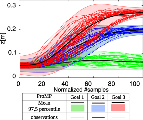
Figure 8. The Cartesian position in the z-axis of the three ProMPs corresponding to reaching three targets. There are 39 trajectory demonstrations per each ProMPs with M = 5 basis functions, $\mathit{\text{c}}=\frac{\text{1}}{\mathit{\text{M}}},\mathit{\text{h}}=\frac{\text{1}}{{\mathit{\text{M}}}^{\text{2}}}$ and $\overline{\mathit{\text{s}}}=\text{100}$.

6.5. Predicting the Desired Movement

Now that we have learned the different ProMPs, we can predict the end of a trajectory according to the early observation n_o. This number is computed from the variable percentData written at the beginning of the trajectory by: $n_o=|\frac{\mathit{\text{percentData}}}{100}\ast t_{\mathit{\text{fi}}}|$, where i is the index of the test trajectory.

To prepare the prediction, the model the time modulation of each trajectory is computed with:

---

1 w = computeAlpha(test.nbData, t, nbInput);

2 promp1.w_alpha = w1;

3 promp2.w_alpha = w2;

4 promp3.w_alpha = w3;

---

This model relies on the global variation of Cartesian position during the first n_o observations. The model’s computations are explained in Section 3.4.

Now, to estimate the time modulation of the trajectory, call the function:

---

1 [alphaTraj, type, x] = inferenceAlpha(promp, test{1}, M, s_bar, c, h, test{1}.nbData, expNoise, ’MO’);

---

where alphaTraj contains the estimated time modulation $\widehat{\alpha }$ and type gives the index of the recognized ProMP. The last parameter x is used for debugging purposes.

Using this estimation of the time modulation, the end of the trajectory is inferred with:

---

1 infTraj = inference(promp, test{1}, M, s_bar, c, h, test{1}.nbData, expNoise, alphaTraj);

---

As shown in the previous example, the quality of the prediction of the future trajectory depends on the accuracy of the time modulation estimation. This estimation is computed by calling the function:

---

1 %Using the model:

2 [alphaTraj, type, x] = inferenceAlpha(promp, test{1}, M, s_bar, c, h, test{1}.nbData, expNoise, ’MO’);

3 %Using the distance criteria:

4 [alphaTraj, type, x] = inferenceAlpha(promp, test{1}, M, s_bar, c, h, test{1}.nbData, expNoise, ’DI’);

5 %Using the Maximum likelihood criteria:

6 [alphaTraj, type, x] = inferenceAlpha(promp, test{1}, M, s_bar, c, h, test{1}.nbData, expNoise, ’ML’);

7 %Using the mean of observed temporal modulation during learning:

8 alphaTraj = (promp{1}.mu_alpha + promp{2}.mu_alpha + promp{3}. mu_alpha)/3.0;

---

6.6. Predicting the Time Modulation

In Section 3.4, we presented four main methods for estimating the time modulation parameter, discussing why this is crucial for a better estimation of the trajectory. Here, we compare the methods on the three goals experiment. We recorded 40 trajectories for each movement primitive, for a total of 120 trajectories. After having computed the corresponding ProMPs, we tested the inference by providing early observations of a trajectory that the robot must finish. For that purpose, it recognizes the correct ProMP among the three precedently learned (see Section 3.5) and then it estimates the time modulation parameter $\widehat{\alpha }$. Figure 9 represents the average error of the $\widehat{\alpha }$ during inference for 10 trials according to the number of observations (from 30 to 90% of observed data) and according to the used method. These methods are the ones we have just presented before that we called mean (equation (11)), maximum likelihood (equation (12)), minimum distance (equation (13)) or model (equation (14)). Each time, the tested trajectory is chosen randomly from the data set of observed trajectories (of course, the test trajectory does not belong to the training set, so it was not used in the learning step). The method that takes the average of α observed during learning is taken as comparison (in black). We can see that other methods are more accurate. The maximum likelihood is increasingly more accurate, as expected. The fourth method (model) that models the α according to the global variation of the trajectory’s positions during the early observations is the best performing when the portion of observed trajectory is small (e.g., 30–50%). Since it is our interest to predict the future trajectory as early as possible, we adopted the model method for our experiments.

FIGURE 9

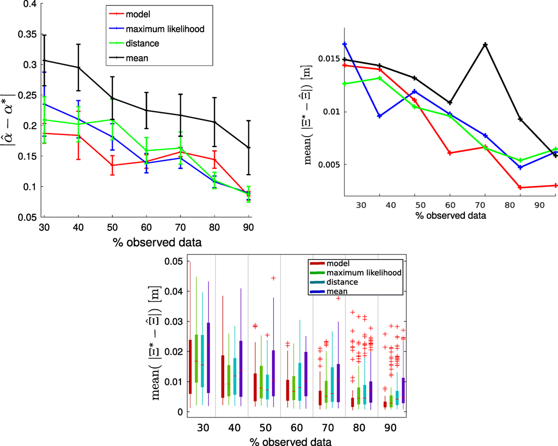
Figure 9. (Top left) Error of α estimation; (top right and bottom) error of trajectory prediction according to the number of known data and the method used. We executed 10 different trials for each case.

7. Application on the Real iCub

In this section, we present and discuss two experiments with the real robot iCub.

In the first, we take inspiration from the experiment of the previous Section 6, where the “tasks” are exemplified by simple point-to-point trajectories demonstrated by a human tutor. In this experiment, we explore how to use wrench information and use known demonstrations as ground truth, to evaluate the quality of our prediction.

In the second experiment, we set up a more realistic collaborative scenario, inspired by collaborative object sorting. In such applications, the robot is used to lift an object (heavy, or dangerous, or that the human cannot manipulate, as for some chemicals or food), the human inspects the object and then decides if it is accepted or rejected. Depending on this decision, the object goes on a tray or bin in front of the robot, or on a bin located on the robot side. Dropping the objects in two cases must be done in a different way. Realizing this application with iCub is not easy, as iCub cannot lift heavy objects and has a limited workspace. Therefore, we simplify the experiment with small objects and two bins. The human simply starts the robots movement with physical guidance, and then the robot finishes the movement on its own. In this experiment the predicted trajectories are validated on-the-fly by the human operator.

In a more complex collaborative scenario, tasks could be elementary tasks such as pointing, grasping, reaching, and manipulating tools (the type of task here is not important, as long as it can be represented by a trajectory).

7.1. Three Simple Actions with Wrench Information

Task trajectories, in this example, have both position and wrench information. In general, it is a good idea to represent collaborative motion primitives in terms of both position and wrenches, as this representation enables using them in the context of physical interaction. Contrarily to the simulated experiment, here the inferred wrenches ${\widehat{F}}_t$ correspond to the wrenches the robot should perceive if the partner was manually guiding the robot to perform the entire movement: indeed, these wrenches are computed from the demonstrations used to learn the primitive. The predicted wrenches can be used in different ways, depending on the application. For example, if the partner breaks the contact with the robot, the perceived wrenches will be different. If the robot is not equipped with tactile or contact sensors, this information can be used by the robot to “perceive” the contact breaking and interpret it, for example, as the sign that the human wants the robot to continue the task on its own. Another use for the demonstrated wrenches is for detecting abnormal forces while the robot is moving: this use can have different applications, from adapting the motion to new environment to automatically detecting new demonstrations. Here, they are simply used to detect when the partner breaks the contact with the robot, and the latter must continue the movement on its own.

In the following, we present how to realize the experiment for predicting the user intention with the real iCub, using our software. The robot must learn three task trajectories represented in Figure 10. In red, the first trajectory goes from an initial position in front of the robot to its left (task A). In green, the second trajectory goes from the same initial position to the top (task C). In blue, the last trajectory goes from the top position to the position on the left (task B).

FIGURE 10

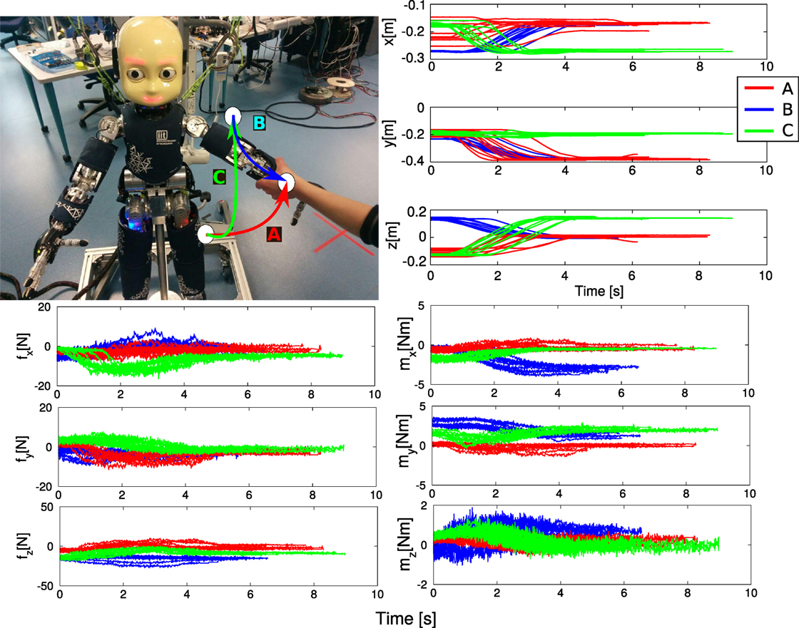
Figure 10. Top left: the iCub and the visualization of the three targets in its workspace, defining the three tasks A–B–C. Top right: Cartesian position information of the demonstrated trajectories for the three tasks. Bottom left and right: wrench (force and moment) information of the demonstrated trajectories.

To provide the demonstrations for the tasks, the human tutor used three visual targets shown on the iCub_GUI, a basic module of the iCub code that provides a real-time synthetic and augmented view of the robot status, with arrows for the external forces and colored objects for the targets. One difficulty for novice users of iCub is to be able to drive the robot’s arm making it perform desired complex 3D trajectories (Ivaldi et al., 2017), but after some practice in moving the robot’s arm the operator recorded all the demonstrations. We want to highlight that having variations in the starting or ending points of the trajectories is not at all a problem, since the ProMPs are able to deal with this variability.

We will see that by using the ProMPs method and by learning the end-effector Cartesian position, the robot will be able to learn distributions over trajectories, recognize when a movement belongs to one of these distributions, and infer the end of the movement.

In this experiment, the robot received 10 demonstrated trajectories per movement primitive, all provided by the same user. We recorded the Cartesian end-effector position and the wrenches of the robot’s left arm. Data are retrieved using the function used_functions/retrieveRealDataWithout Orientation.m. The output parameters of this function are three objects (one per ProMP) that contain all the required information to learn the ProMPs.

In this function, the wrench information are filtered using a Matlab function called envelope.m ¹⁵: for each trajectory trajand its subMatrix M = F([1: t]):

---

1 [envHigh, envLow] = envelope(traj.M);

2 traj.M = (envHigh + envLow)/2;

---

These three objects are saved in ’Data/realIcub.mat’. A Matlab script called demo_plotProMPsIcub.m recovers these data, using the function load(’Data/realIcub.mat’). This script follows the same organization as the ones we previously explained in Sections 5 and 6. By launching this script, the recovered data are plotted first.

Then, the ProMPs are computed and plotted, as presented in Figure 11. In this figure, the distributions are visibly overlaid:

• during the whole trajectories duration for the wrench information;

• during the 40% first samples of the trajectories for the Cartesian position information.

FIGURE 11

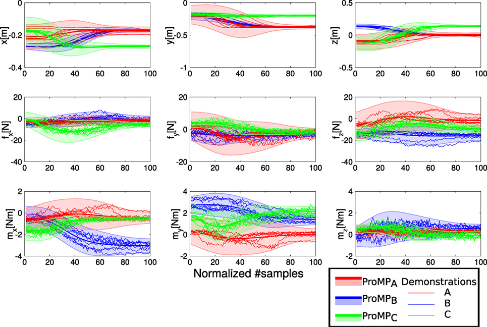
Figure 11. The ProMPs learned by the robot from the demonstrations of Figure 10.

After this learning step, the user chooses which ProMP to test. Using a variable that represents the percentage of observed data to be used for the inference, the script computes the number of early observations n_o¹⁶ that will be measured by the robot. Using this number, the robot models the time modulation parameter α¹⁷ of each ProMP, as explained in Section 3.4. Using this model, the time modulation of the test trajectory is estimated, and the corresponding ProMP is identified.

Then, the inference of the trajectory’s target is performed. Figure 12 represents the inference of the three tested trajectories when wrench information is not used by the robot to infer the trajectory. To realize this figure, with the comparison between the predicted trajectory and the ground truth, we applied our algorithm offline. In fact, it is not possible at time t to have the ground truth of the trajectory intended by the human from t + 1 to t_f: even if we would tell to the human in advance the goal that he/she must reach for, the trajectory to reach that goal could vary. So, for the purpose of these figures and comparisons with the ground truth, we show here the offline evaluation: we select one demonstrated task trajectory from the test set (not the training set used to learn the ProMP) as ground truth, and imagine that this is the intended trajectory. In Figure 12, the ground truth is shown in black, whereas the portion of this trajectory that is fed to the inference, and that corresponds to the “early observations,” is represented with bigger black circles. We can see that the inference of the Cartesian position is correct, although we can see an error of about 1 s of the estimated duration time for the last trial. Also, the wrench inference is not accurate. We can assume that it is: because the robot infers the trajectory using only position information without wrench information, or because the wrenches’ variation is not correlated to the position variation. To improve this result, we can make the inference using wrench in addition to Cartesian position information, as shown in Figure 13. We can see in this figure that the estimation of the trajectory’s duration is accurate. The disadvantage is that the inference of the Cartesian position is less accurate because the posterior distribution computation makes a trade-off between fitting Cartesian position and wrench early observations. Moreover, to allow a correct inference using wrench information, the noise expectation must be increased to consider forces.¹⁸

FIGURE 12

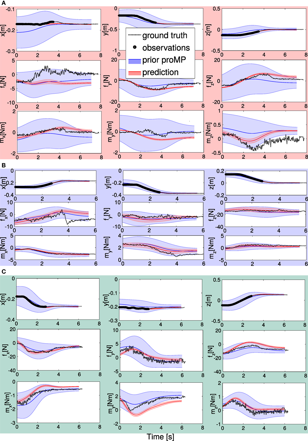
Figure 12. The prediction of the future trajectory from the learned ProMPs computed from the position information for the 3-targets dataset on the real iCub (Figure 11) after 40% of observations.

FIGURE 13

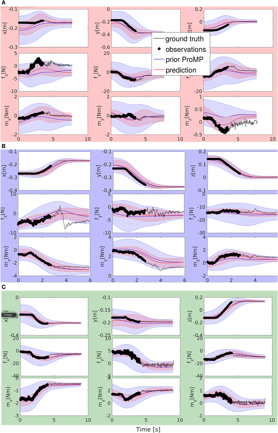
Figure 13. The prediction of the future trajectory from the learned ProMPs computed from the position and wrench information for the 3-targets dataset on the real iCub (Figure 11) after 40% of observations.

To confirm these results, we analyzed the trajectory inference and α estimation considering different percentages of each trajectory as observed data (30–90%). For each percentage, we performed 20 tests, with and without force information.

In Figure 14, each box-plot represents errors for 20 tests. On the top, the error criterion is the average distance between the inferred trajectory and the real one. We can see that the inference of Cartesian end-effector trajectory is more accurate without wrench information. On the bottom, the error criterion is the distance between the estimated α and the real one. We can see that using wrench information, the estimation of the α is more accurate. Thus, these two graphs confirm what we assumed from Figures 12 and 13.

FIGURE 14

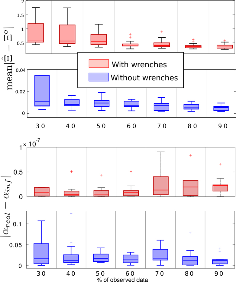
Figure 14. Trajectory prediction error (top) and time modulation estimation error (bottom) of the future trajectory with and without wrench information, for the 3-targets dataset on the real iCub (Figure 11) with respect to the number of observed data points.

Median, mean, and variance of the prediction errors, computed with the normalized root-mean-square error (NRMSE), are reported in Table S1 in Supplementary Material. The prediction error for the time modulation is a scalar: |α_prediction − α_real|. The prediction error for the trajectory is computed by the NRMSE of |Ξ_prediction − Ξ_real|.

In future upgrades for this application, we will probably use the wrench information only to estimate the time modulation parameter α, to have both the best inference of the intended trajectory and the best estimation of the time modulation parameter to combine the benefits of inference with and without wrench information.

Table S1 in Supplementary Material also reports the average time for computing the prediction of both time modulation and posterior distribution. The computation was performed in Matlab, on a single core laptop (no parallelization). While the computation time for the case “without wrenches” is fine for real-time application, using the wrench information delays the prediction and represents a limit for real-time applications if fast decisions have to taken by the robot. Computation time will be improved in the future works, with the implementation of the prediction in an iterative way.

7.2. Collaborative Object Sorting

We realized another experiment with iCub, where the robot has to sort some objects in different bins (see Figure S2 in Supplementary Material). We have two main primitives: one for a bin located on the left of the robot, and one for the bin to the front. Dropping the object is done at different heights, with a different gesture that also has a different orientation of the hand. For this reason, the ProMP model consists of the Cartesian position of the hand X_t = [x_t, y_t, z_t] ∈ R³ and its orientation A_t ∈ R⁴, expressed as a quaternion:

${\xi }_t=\left[\begin{array}{c}\hfill X_t\hfill \\ \hfill A_t\hfill \end{array}\right]={\mathrm{\Phi }}_{\alpha t}\omega +{\epsilon }_t.$

As in the previous experiment, we first teach the robot the primitives by kinesthetic teaching, with a dozen of demonstrations. Then we start the robot movement: the human operator physically grabs the robot’s arm and start the movement toward one of the bins. The robot’s skin is used twice. First, to detect the contact when the human grabs the arm, which marks the beginning of the observations. Second, when the human breaks the contact with the arm, which marks the end of the observations. Using the first portion of the observed movement, the robot recognizes the current task that is being executed, predicts the future movement that is intended by the human, and then executes it on its own. In the video (see link in Section 8), we artificially introduced a pause to let the operator “validate” the predicted trajectory, using a visual feedback on the iCubGui. Figure S3 in Supplementary Material shows one of the predictions made by the robot after the human releases the arm. Of course in this case, we do not have a “ground truth” for the predicted trajectory, only a validation of the predicted trajectory by the operator.

8. Videos

We recorded several videos that complement the tutorials. The videos are presented in the github repository of our software: https://github.com/inria-larsen/icubLearningTrajectories/tree/master/Videos.

9. Discussion

While we believe that our proposed method is principled and has several advantages for predicting intention in human–robot interaction, there are numerous improvements that can be done. Some will be object of our future works.

9.1. Improving the Estimation of the Time Modulation

Our experiments showed that estimating the time modulation parameter α, determining the duration of the trajectory, greatly improves the prediction of the trajectory in terms of difference with the human intended trajectory (i.e., our ground truth). We proposed four simple methods in Section 3.4, and in the iCub experiment, we showed that the method that maps the time modulation and the variation of the trajectory in the first n_o observations provides a good estimate of the time modulation α for our specific application. However, it is an ad hoc model that cannot be generalized to all possible cases. Overall, the estimation of the time modulation (or phase) can be improved. For example, Maeda et al. (2016) used Dynamic Time Warping, while Ewerton et al. (2015) proposed to improve the estimation by having local estimations of the speed in the execution of the trajectory, to comply with cases where the velocity of task trajectory may not be constant throughout the task execution. In the future, we plan to explore more solutions and integrate them into our software.

9.2. Improving Prediction

Another point that needs further investigation and improvement is how to improve the prediction of the trajectories exploiting different information. In our experiment with iCub, we improved the estimation of the time modulation using position and wrench information; however, we observed that the noisy wrench information does not help in improving the prediction of the position trajectory. One improvement is to certainly exploit more information from the demonstrated trajectories, such as estimating the different noise of every trajectory component and exploiting this information to improve the prediction. Another possible improvement would consist in using contextual information about the task trajectories. Finally, it would be interesting to try to identify automatically the characteristic such as velocity profiles or accelerations, which are renown to play a key role in attributing intentions to human movements. For example, in goal-directed tasks such as reaching, the arm velocity profile, and the hand configuration are cues that helps us detect intentions. Extracting these cues automatically, leveraging the estimation of the time modulation, would probably improve the prediction of the future trajectory. This is a research topic on its own, outside the scope of this article, with strong links to human motor control.

9.3. Continuous Prediction

In Section 3.5, we described how to compute the prediction of the future trajectory after recognizing the current task. However, we did not explore what happens if the task recognition is wrong: this may happen, if there are two or more task with a similar trajectory at the beginning (e.g., moving the object from the same initial point toward one of four possible targets), or simply because there were not enough observed points. So what happens if our task recognition is wrong? How to re-decide on a previously identified task? And how should the robot decide if its current prediction is finally correct (in statistical terms)? While implementing a continuous recognition and prediction is easy with our framework (one has simply to do the estimation at each time step), providing a generic answer to these question may not be straightforward. Re-deciding about the current task implies also changing the prediction of the future trajectory. If the decision does not come with a confidence level greater than a desired value, then the robot could face a stall: if asked to continue the movement but unsure about the future trajectory, should it continue or stop? The choice may be application dependent. We will address these issues and the continuous prediction in future works.

9.4. Improving Computational Time

Finally, we plan to improve the computational time for the inference and the portability of our software by porting the entire framework in C++.

9.5. Learning Tasks with Objects

In many collaborative scenarios, such as object carrying and cooperative assembly, the physical interaction between the human and the robot is mediated by objects. In these cases, if specific manipulations must be done on the objects, our method still applies, but not only on the robot. It must be adapted to the new “augmented system” consisting of robot and object. Typically, we could image a trajectory for some frame or variable or point of interest for the object and learn the corresponding task. Since ProMPs support multiplication and sequencing of primitives, we could exploit the properties of the ProMPs to learn the joint distribution of the robot task trajectories and the object task trajectories.

10. Conclusion

In this article, we propose a method for predicting the intention of a user physically interacting with the iCub in a collaborative task. We formalize the intention prediction as predicting the target and “future” intended trajectory from early observations of the task trajectory, modeled by Probabilistic Movement Primitives (ProMPs). We use ProMPs because they capture the variability of the task, in the form of a distribution of trajectories coming from several demonstrations of the task. From the information provided by the ProMP, we are able to compute the future trajectory by conditioning the ProMP to match the early observed data points. Additional features of our method are the estimation of the duration of the intended movement, the recognition of the current task among the many known in advance, and multimodal prediction.

Section 3 described the theoretical framework, whereas Sections 4–7 presented the open-source software that provides the implementation of the proposed method. The software is available on github, and tutorials and videos are provided.

We used three examples of increasing complexity to show how to use our method for predicting the intention of the human in collaborative tasks, exploiting the different features. We presented experiments with both the real and the simulated iCub. In our experiments, the robot learns a set of motion primitives corresponding to different tasks, from several demonstrations provided by a user. The resulting ProMPs are the prior information that is later used to make inferences about human intention. When the human starts a new collaborative task, the robot uses the early observations to infer which task the human is executing and predicts the trajectory that the human intends to execute. When the human releases the robot, the predicted trajectory is used by the robot to continue executing the task on its own.

In Section 9, we discussed some current issues and challenges for improving the proposed method and make it applicable to a wider repertoire of collaborative human–robot scenarios. In our future works, our priority would be in accelerating the time for computing the inference and finding a principled way to do continuous estimation, by letting the robot re-decide continuously about the current task and future trajectory.

Author Contributions

Designed study: OD, AP, FC, and SI. Wrote software: OD, ME, AP, and SI. Wrote paper: OD, AP, ME, FC, JP, and SI.

Conflict of Interest Statement

The authors declare that the research was conducted in the absence of any commercial or financial relationships that could be construed as a potential conflict of interest.

Acknowledgments

The authors wish to thank the IIT researchers of the CoDyCo project for their support with iCub, Ugo Pattacini and Olivier Rochel for their help with the software for the Geomagic, and Iñaki Fernández Pérez for all his relevant feedback.

Funding

This study was partially funded by the European projects CoDyCo (no. 600716 ICT211.2.1) and AnDy (no. 731540 H2020-ICT-2016-1) and the French CPER project SCIARAT.

Supplementary Material

The Supplementary Material for this article can be found online at https://www.frontiersin.org/article/10.3389/frobt.2017.00045/full#supplementary-material.

Footnotes

1. ^Currently, this scenario is frequently addressed in manufacturing by robots and lifters; in the future, we imagine that humanoid robots could also be used for such task, for assisting workers in environments where robots cannot be installed on a fixed base, such as in some aircraft manufacturing operations (Caron and Kheddar, 2016).
2. ^There may be applications where converging to a unique and precise goal could be a desirable property of the robot’s movement. However, it is an assumption that prevents us to generalize the method for different actions, and this is another reason why we prefer ProMPs.
3. ^We refer the interested reader to Maeda et al. (2014) for a thorough comparison between DMPs and ProMPs to be used for interaction primitives and prediction.
4. ^To avoid disambiguation, in our method, tasks are encoded by primitives that are made of trajectories: this is a very classical approach for robot learning techniques and in general techniques based on primitives. Of course this is a simplification, but it allows representing a number of different tasks: pointing, reaching, grasping, gazing, etc.
5. ^In this article, we denote by early observations the first portion of a movement observed by the robot, i.e., from t = 0 to acurrent t.
6. ^The Geomagic Touch is a haptic device, capable of providing force feedback from the simulation to the operator. In our experiments with the simulated iCub, we did not use this feature. We used the Geomagic Touch to steer the arm of the simulated robot. In that sense, we used it more as a joystick for moving the left arm.
7. ^In some tasks, e.g., reaching, it is reasonable to assume that the difference of duration of the demonstrated trajectories is negligible; however, in other tasks, the duration of the demonstrated trajectories may vary significantly.
8. ^That is, we computed the p(ω) distribution from the dataset $\left\{\omega {}_1,\dots ,\omega {}_n\right\}$, where each ω_i is an estimated parameter computed from the trajectory demonstrations.
9. ^Actually, we call here duration what is in fact the total number of samples for the trajectory.
10. ^In our case, this assumption can be appropriate, because the reaching trajectories in our application are generally monotonic increasing/decreasing.
11. ^In this model, we assume that we can find the time modulation parameter according to the global variation of the position during the n_o first observed data.
12. ^Note that in that particular example we do not use the orientation because we want the robot’s hand to keep the same orientation during the movement. But in principle, it is possible to learn trajectories consisting of the 6D/7D Cartesian position and orientation of the hand, to make the robot change also the orientation of the hand during the task.
13. ^In our example, we do not use the simulated wrench information as it is very noisy. However, we provide the code and show how to retrieve it and use it, in case the readers should not have access to the real iCub.
14. ^Note that in our example wrenches are separated from the Cartesian position, because they are not used to recognize the index of the current ProMP during the inference.
15. ^Information about this function can be found here: https://fr.mathworks.com/help/signal/ref/envelope.html?requestedDomain=www.mathworks.com.
16. ^n_o is not the same for each trajectory test, because it depends on the total duration of the trajectory to be inferred.
17. ^Since the model uses the n_o parameter, its computation cannot be performed before this step.
18. ^In future versions, we will include the possibility to have different noise models for the observations, e.g., we will have ${\Sigma }_{\Xi }^o=\left[\begin{array}{cc}\hfill {\Sigma }_X\hfill & \hfill 0\hfill \\ \hfill 0\hfill & \hfill {\Sigma }_F\hfill \end{array}\right]$. We will therefore set a bigger covariance for the wrench information than for the position information.
19. ^From the book (Bishop, 2006).

References

Alami, R., Clodic, A., Montreuil, V., Sisbot, E. A., and Chatila, R. (2006). “Toward human-aware robot task planning,” in AAAI Spring Symposium: To Boldly Go Where No Human-Robot Team Has Gone Before, Beijing, 39–46.

Google Scholar

Amor, H. B., Neumann, G., Kamthe, S., Kroemer, O., and Peters, J. (2014). “Interaction primitives for human-robot cooperation tasks,” in Robotics and Automation (ICRA), 2014 IEEE International Conference on (Hong Kong: IEEE), 2831–2837.

Google Scholar

Baraglia, J., Cakmak, M., Nagai, Y., Rao, R., and Asada, M. (2016). “Initiative in robot assistance during collaborative task execution,” in Human-Robot Interaction (HRI), 2016 11th ACM/IEEE International Conference on (Christchurch: IEEE), 67–74.

Google Scholar

Billard, A., and Mataric, M. J. (2001). Learning human arm movements by imitation: evaluation of a biologically inspired connectionist architecture. Rob. Auton. Syst. 37, 145–160. doi: 10.1016/S0921-8890(01)00155-5

CrossRef Full Text | Google Scholar

Bishop, C. M. (2006). Pattern Recognition and Machine Learning (Information Science and Statistics). Secaucus, NJ: Springer-Verlag New York, Inc.

Google Scholar

Busch, B., Grizou, J., Lopes, M., and Stulp, F. (2017). Learning legible motion from human–robot interactions. Int. J. Soc. Robot. 1–15. doi:10.1007/s12369-017-0400-4

CrossRef Full Text | Google Scholar

Buxton, H. (2003). Learning and understanding dynamic scene activity: a review. Image Vision Comput. 21, 125–136. doi:10.1016/S0262-8856(02)00127-0

CrossRef Full Text | Google Scholar

Calinon, S. (2015). pbdlib-matlab. Available at: https://gitlab.idiap.ch/rli/pbdlib-matlab/

Google Scholar

Calinon, S. (2016). A tutorial on task-parameterized movement learning and retrieval. Intell. Serv. Robot. 9, 1–29. doi:10.1007/s11370-015-0187-9

CrossRef Full Text | Google Scholar

Calinon, S., Bruno, D., and Caldwell, D. G. (2014). “A task-parameterized probabilistic model with minimal intervention control,” in IEEE International Conference on Robotics and Automation (ICRA), Hong Kong, 3339–3344.

Google Scholar

Calinon, S., Li, Z., Alizadeh, T., Tsagarakis, N. G., and Caldwell, D. G. (2012a). Statistical Dynamical Systems for Skills Acquisition in Humanoids. Available at: http://www.calinon.ch/showPubli.php?publi=3031

Google Scholar

Calinon, S., Li, Z., Alizadeh, T., Tsagarakis, N. G., and Caldwell, D. G. (2012b). “Statistical dynamical systems for skills acquisition in humanoids,” in Proc. IEEE Intl Conf. on Humanoid Robots (Humanoids), Osaka, Japan, 323–329.

Google Scholar

Carlson, T., and Demiris, Y. (2008). “Human-wheelchair collaboration through prediction of intention and adaptive assistance,” in Robotics and Automation, 2008. ICRA 2008. IEEE International Conference on (Pasadena: IEEE), 3926–3931.

Google Scholar

Caron, S., and Kheddar, A. (2016). “Multi-contact walking pattern generation based on model preview control of 3d com accelerations,” in Humanoid Robots, 2016 IEEE-RAS International Conference on, Cancun.

Google Scholar

Csibra, G., and Gergely, G. (2007). ‘Obsessed with goals’: functions and mechanisms of teleological interpretation of actions in humans. Acta Psychol. 124, 60–78. doi:10.1016/j.actpsy.2006.09.007

PubMed Abstract | CrossRef Full Text | Google Scholar

Demiris, Y. (2007). Prediction of intent in robotics and multi-agent systems. Cogn. Process. 8, 151–158. doi:10.1007/s10339-007-0168-9

PubMed Abstract | CrossRef Full Text | Google Scholar

Dermy, O. (2017). icubLearningTrajectories. Available at: https://github.com/inria-larsen/icubLearningTrajectories

Google Scholar

DeWolf, T. (2013). pydmps. Available at: https://github.com/studywolf/pydmps

Google Scholar

Dragan, A., and Srinivasa, S. (2013). “Generating legible motion,” in Proceedings of Robotics: Science and Systems, Berlin, Germany.

Google Scholar

Dragan, A., and Srinivasa, S. (2014). Integrating human observer inferences into robot motion planning. Auton. Robots 37, 351–368. doi:10.1007/s10514-014-9408-x

CrossRef Full Text | Google Scholar

Dumora, J., Geffard, F., Bidard, C., Aspragathos, N. A., and Fraisse, P. (2013). “Robot assistance selection for large object manipulation with a human,” in IEEE International Conference on Systems, Man, and Cybernetics, Manchester, 1828–1833.

Google Scholar

Evrard, P., Gribovskaya, E., Calinon, S., Billard, A., and Kheddar, A. (2009). “Teaching physical collaborative tasks: object-lifting case study with a humanoid,” in Humanoid Robots, 2009. Humanoids 2009. 9th IEEE-RAS International Conference on (Paris: IEEE), 399–404.

Google Scholar

Ewerton, M. (2016). Learning Motor Skills from Partially Observed Movements Executed at Different Speeds. Available at: https://github.com/studywolf/pydmps

Google Scholar

Ewerton, M., Neumann, G., Lioutikov, R., Ben Amor, H., Peters, J., and Maeda, G. (2015). “Learning multiple collaborative tasks with a mixture of interaction primitives,” in Robotics and Automation (ICRA), 2015 IEEE International Conference on (Seattle: IEEE), 1535–1542.

Google Scholar

Ferrer, G., and Sanfeliu, A. (2014). Bayesian human motion intentionality prediction in urban environments. Pattern Recognit. Lett. 44, 134–140. doi:10.1016/j.patrec.2013.08.013

CrossRef Full Text | Google Scholar

Fine, S., Singer, Y., and Tishby, N. (1998). The hierarchical hidden Markov model: analysis and applications. Mach. Learn. 32, 41–62. doi:10.1023/A:1007469218079

CrossRef Full Text | Google Scholar

Fitts, P. M. (1992). The information capacity of the human motor system in controlling the amplitude of movement. J. Exp. Psychol. Gen. 121, 262. doi:10.1037/0096-3445.121.3.262

CrossRef Full Text | Google Scholar

Fumagalli, M., Ivaldi, S., Randazzo, M., Natale, L., Metta, G., Sandini, G., et al. (2012). Force feedback exploiting tactile and proximal force/torque sensing. Auton. Robots 33, 381–398. doi:10.1007/s10514-012-9291-2

CrossRef Full Text | Google Scholar

Gribovskaya, E., Kheddar, A., and Billard, A. (2011). “Motion learning and adaptive impedance for robot control during physical interaction with humans,” in Robotics and Automation (ICRA), 2011 IEEE International Conference on (Shanghai: IEEE), 4326–4332.

Google Scholar

Hersch, M., Guenter, F., Calinon, S., and Billard, . (2008). Dynamical System Modulation for Robot Adaptive Learning via Kinesthetic Demonstrations. Available at: http://lasa.epfl.ch/sourcecode/counter.php?ID=11&index=1

Google Scholar

Hoffman, G. (2010). “Anticipation in human-robot interaction,” in AAAI Spring Symposium: It’s All in the Timing, Palo Alto, CA.

Google Scholar

Huang, S. H., Held, D., Abbeel, P., and Dragan, A. D. (2017). Enabling robots to communicate their objectives. CoRR. abs/1702.03465. Available at: http://arxiv.org/abs/1702.03465

Google Scholar

Ijspeert, A. J., Nakanishi, J., Hoffmann, H., Pastor, P., and Schaal, S. (2013). Dynamical movement primitives: learning attractor models for motor behaviors. Neural Comput. 25, 328–373. doi:10.1162/NECO_a_00393

PubMed Abstract | CrossRef Full Text | Google Scholar

Ivaldi, S., Anzalone, S., Rousseau, W., Sigaud, O., and Chetouani, M. (2014a). Robot initiative in a team learning task increases the rhythm of interaction but not the perceived engagement. Front. Neurorobot. 8:5. doi:10.3389/fnbot.2014.00005

CrossRef Full Text | Google Scholar

Ivaldi, S., Nguyen, S. M., Lyubova, N., Droniou, A., Padois, V., Filliat, D., et al. (2014b). Object learning through active exploration. IEEE Trans. Auton. Ment. Dev. 6, 56–72. doi:10.1109/TAMD.2013.2280614

CrossRef Full Text | Google Scholar

Ivaldi, S., Fumagalli, M., Nori, F., Baglietto, M., Metta, G., and Sandini, G. (2010). “Approximate optimal control for reaching and trajectory planning in a humanoid robot,” in Proc. of the 2010 IEEE/RSJ International Conference on Intelligent Robots and Systems – IROS, Taipei, Taiwan, 1290–1296.

Google Scholar

Ivaldi, S., Fumagalli, M., Randazzo, M., Nori, F., Metta, G., and Sandini, G. (2011). “Computing robot internal/external wrenches by means of inertial, tactile and f/t sensors: theory and implementation on the icub,” in Humanoid Robots (Humanoids), 2011 11th IEEE-RAS International Conference on (Bled: IEEE), 521–528.

Google Scholar

Ivaldi, S., Lefort, S., Peters, J., Chetouani, M., Provasi, J., and Zibetti, E. (2017). Towards engagement models that consider individual factors in HRI: on the relation of extroversion and negative attitude towards robots to gaze and speech during a human-robot assembly task. Int. J. Soc. Robot. 9, 63–86. doi:10.1007/s12369-016-0357-8

CrossRef Full Text | Google Scholar

Jamone, L., Ugur, E., Cangelosi, A., Fadiga, L., Bernardino, A., Piater, J., et al. (2017). Affordances in psychology, neuroscience and robotics: a survey. IEEE Trans. Cognit. Dev. Syst. 99, 1. doi:10.1109/TCDS.2016.2594134

CrossRef Full Text | Google Scholar

Jarrassé, N., Paik, J., Pasqui, V., and Morel, G. (2008). “How can human motion prediction increase transparency?,” in Robotics and Automation, 2008. ICRA 2008. IEEE International Conference on (Pasadena, CA: IEEE), 2134–2139.

Google Scholar

Keogh, E. (2002). “Exact indexing of dynamic time warping,” in Proceedings of the 28th International Conference on Very Large Data Bases (Hong Kong: VLDB Endowment), 406–417.

Google Scholar

Khansari, M. (2011). Dynamical Systems Approach to Learn Robot Motions. Available at: https://bitbucket.org/khansari/seds

Google Scholar

Khansari-Zadeh, S. M., and Billard, A. (2011). Learning stable nonlinear dynamical systems with gaussian mixture models. IEEE Trans. Robot. 27, 943–957. doi:10.1109/TRO.2011.2159412

CrossRef Full Text | Google Scholar

Khansari-Zadeh, S. M., and Billard, A. (2012). A dynamical system approach to realtime obstacle avoidance. Auton. Robots 32, 433–454. doi:10.1007/s10514-012-9287-y

CrossRef Full Text | Google Scholar

Kim, J., Banks, C. J., and Shah, J. A. (2017). “Collaborative planning with encoding of users’ high-level strategies,” in AAAI Conference on Artificial Intelligence (AAAI-17), San Francisco, CA.

Google Scholar

Langolf, G. D., Chaffin, D. B., and Foulke, J. A. (1976). An investigation of fitts? Law using a wide range of movement amplitudes. J. Mot. Behav. 8, 113–128. doi:10.1080/00222895.1976.10735061

CrossRef Full Text | Google Scholar

Lober, R. (2014). Stochastic Machine Learning Toolbox. Available at: https://github.com/rlober/smlt

Google Scholar

Lober, R., Padois, V., and Sigaud, O. (2014). “Multiple task optimization using dynamical movement primitives for whole-body reactive control,” in Humanoid Robots (Humanoids), 2014 14th IEEE-RAS International Conference on (Madrid: IEEE), 193–198.

Google Scholar

Maeda, G., Ewerton, M., Lioutikov, R., Ben Amor, H., Peters, J., and Neumann, G. (2014). “Learning interaction for collaborative tasks with probabilistic movement primitives,” in Humanoid Robots (Humanoids), 2014 14th IEEE-RAS International Conference on (Madrid: IEEE), 527–534.

Google Scholar

Maeda, G. J., Neumann, G., Ewerton, M., Lioutikov, R., Kroemer, O., and Peters, J. (2016). “Probabilistic movement primitives for coordination of multiple human–robot collaborative tasks,” in Autonomous Robots, 1–20.

Google Scholar

Meier, F., and Schaal, S. (2016). A probabilistic representation for dynamic movement primitives. CoRR. abs/1612.05932. Available at: http://arxiv.org/abs/1612.05932

Google Scholar

Micha, H., and Aude, B. (2008). Dynamical system modulation for robot learning via kinesthetic demonstrations. IEEE Trans. Robot. 24, 1463–1467. doi:10.1109/TRO.2008.2006703

CrossRef Full Text | Google Scholar

Nguyen, N. T., Phung, D. Q., Venkatesh, S., and Bui, H. (2005). “Learning and detecting activities from movement trajectories using the hierarchical hidden Markov model,” in Computer Vision and Pattern Recognition, 2005. CVPR 2005. IEEE Computer Society Conference on, Vol. 2 (San Diego, CA: IEEE), 955–960.

Google Scholar

Palinko, O., Sciutti, A., Patané, L., Rea, F., Nori, F., and Sandini, G. (2014). “Communicative lifting actions in human-humanoid interaction,” in Humanoid Robots (Humanoids), 2014 14th IEEE-RAS International Conference on (Madrid: IEEE), 1116–1121.

Google Scholar

Paraschos, A., Daniel, C., Peters, J. R., and Neumann, G. (2013a). “Probabilistic movement primitives,” in Advances in Neural Information Processing Systems, Stateline, NV, 2616–2624.

Google Scholar

Paraschos, A., Neumann, G., and Peters, J. (2013b). “A probabilistic approach to robot trajectory generation,” in Humanoid Robots (Humanoids), 2013 13th IEEE-RAS International Conference on (Atlanta, GA: IEEE), 477–483.

Google Scholar

Paraschos, A., Rueckert, E., Peters, J., and Neumann, G. (2015). “Model-free probabilistic movement primitives for physical interaction,” in Intelligent Robots and Systems (IROS), 2015 IEEE/RSJ International Conference on (Hamburg: IEEE), 2860–2866.

Google Scholar

Pattacini, U., Nori, F., Natale, L., Metta, G., and Sandini, G. (2010). “An experimental evaluation of a novel minimum-jerk cartesian controller for humanoid robots,” in Intelligent Robots and Systems (IROS), 2010 IEEE/RSJ International Conference on (Taipei: IEEE), 1668–1674.

Google Scholar

Peters, J., Lee, D. D., Kober, J., Nguyen-Tuong, D., Bagnell, J. A., and Schaal, S. (2016). “Robot learning,” in Springer Handbook of Robotics, 357–398.

Google Scholar

Ren, H., and Xu, G. (2002). “Human action recognition with primitive-based coupled-HMM,” in Pattern Recognition, 2002. Proceedings. 16th International Conference on, Vol. 2 (Quebec: IEEE), 494–498.

Google Scholar

Rozo Castañeda, L., Calinon, S., Caldwell, D., Jimenez Schlegl, P., and Torras, C. (2013). “Learning collaborative impedance-based robot behaviors,” in Proceedings of the Twenty-Seventh AAAI Conference on Artificial Intelligence, 1422–1428.

Google Scholar

Sahin, E., Çakmak, M., Dogar, M. R., Ugur, E., and Üçoluk, G. (2007). To afford or not to afford: a new formalization of affordances toward affordance-based robot control. Adapt. Behav. 15, 447–472. doi:10.1177/1059712307084689

CrossRef Full Text | Google Scholar

Sato, T., Nishida, Y., Ichikawa, J., Hatamura, Y., and Mizoguchi, H. (1994). “Active understanding of human intention by a robot through monitoring of human behavior,” in Proceedings of the IEEE/RSJ/GI International Conference on Intelligent Robots and Systems, Vol. 1, Munich, 405–414.

Google Scholar

Schaal, S. (2006). “Dynamic movement primitives: a framework for motor control in humans and humanoid robotics,” in Adaptive Motion of Animals and Machines Springer, 261–280.

Google Scholar

Sciutti, A., Bisio, A., Nori, F., Metta, G., Fadiga, L., and Sandini, G. (2013). Robots can be perceived as goal-oriented agents. Interact. Stud. 14, 329–350. doi:10.1075/is.14.3.02sci

CrossRef Full Text | Google Scholar

Shah, J., Wiken, J., Williams, B., and Breazeal, C. (2011). “Improved human-robot team performance using chaski, a human-inspired plan execution system,” in Proceedings of the 6th International Conference on Human-Robot Interaction (Lausanne: ACM), 29–36.

Google Scholar

Silva, D. F., and Batista, G. E. (2016). “Speeding up all-pairwise dynamic time warping matrix calculation,” in Proceedings of the 2016 SIAM International Conference on Data Mining (Miami, FL: SIAM), 837–845.

Google Scholar

Soechting, J. (1984). Effect of target size on spatial and temporal characteristics of a pointing movement in man. Exp. Brain Res. 54, 121–132. doi:10.1007/BF00235824

PubMed Abstract | CrossRef Full Text | Google Scholar

Soh, H., and Demiris, Y. (2015). Learning assistance by demonstration: smart mobility with shared control and paired haptic controllers. J. Hum. Robot Interact. 4, 76–100. doi:10.5898/JHRI.4.3.Soh

CrossRef Full Text | Google Scholar

Stulp, F. (2014). DmpBbo – a c++ Library for Black-Box Optimization of Dynamical Movement Primitives. Available at: https://github.com/stulp/dmpbbo

Google Scholar

Stulp, F., Raiola, G., Hoarau, A., Ivaldi, S., and Sigaud, O. (2013). “Learning compact parameterized skills with a single regression,” in Proc. IEEE-RAS International Conference on Humanoid RObots – HUMANOIDS, Atlanta, GA, 1–7.

Google Scholar

Thill, S., and Ziemke, T. (2017). “The role of intention in human-robot interaction,” in Proceedings of the Companion of the 2017 ACM/IEEE International Conference on Human-Robot Interaction, HRI ’17 (New York, NY, USA: ACM), 427–428.

Google Scholar

Wang, J. M., Fleet, D. J., and Hertzmann, A. (2005). “Gaussian process dynamical models,” in NIPS, Vol. 18, Vancouver, 3.

Google Scholar

Wang, Z., Deisenroth, M. P., Amor, H. B., Vogt, D., Schölkopf, B., and Peters, J. (2012). “Probabilistic modeling of human movements for intention inference,” in Robotics: Science and Systems (Sydney, NSW: Citeseer).

Google Scholar

Wang, Z., Mülling, K., Deisenroth, M. P., Amor, H. B., Vogt, D., Schölkopf, B., et al. (2013). Probabilistic movement modeling for intention inference in human-robot interaction. Int. J. Robot. Res. 32, 841–858. doi:10.1177/0278364913478447

CrossRef Full Text | Google Scholar

Zube, A., Hofmann, J., and Frese, C. (2016). “Model predictive contact control for human-robot interaction,” in Proceedings of ISR 2016: 47st International Symposium on Robotics, Munich, 1–7.

Google Scholar

Appendix

A. Detail of the Inference Formula

In this Appendix, we explain how to obtain the inference formulae used in our software. First, let us recall the Marginal and Conditional Gaussians laws.¹⁹ Given a marginal Gaussian distribution for x and a Gaussian distribution for y given x in the following form:

$p\left(x\right)=\mathcal{N}\left(x|\mu ,{\mathrm{\Delta }}^{-1}\right)p\left(y|x\right)=\mathcal{N}\left(\mathit{\text{Ax}}+b,L^{-1}\right),$ (A1)

the marginal distribution of y and the conditional distribution of x given y are given by the following equations:

$\begin{array}{l}\hfill p\left(y\right)=\mathcal{N}\left(y|A\mu +b,L^{-1}+A{\mathrm{\Delta }}^{-1}{A}^{\top }\right),\end{array}$ (A2)

$\begin{array}{l}\hfill p\left(x|y\right)=\mathcal{N}\left(x|\Sigma A^{\top }L\left(y-b\right)+\mathrm{\Delta }\mu ,\Sigma \right),\end{array}$ (A3)

where

$\Sigma ={\left(\mathrm{\Delta }+A^{\text{T}}\mathit{\text{LA}}\right)}^{-1}.$

We computed the parameter’s marginal Gaussian distribution from the set of observed movements:

$p\left(\omega \right)\sim \mathcal{N}\left({\mu }_{\omega },{\Sigma }_{\omega }\right),$ (A4)

From the model ${\Xi }_t={\mathrm{\Phi }}_{\left[1:t_f\right]}\omega +{\epsilon }_{\Xi }$, we have the conditional Gaussian distribution for Ξ given ω:

$p\left(\Xi |\omega \right)=\mathcal{N}\left(\Xi |{\mathrm{\Phi }}_{\left[1:t_f\right]}\omega ,{\Sigma }_{\Xi }\right).$ (A5)

Then, using equation (A2) we have the following:

$p\left(\Xi \right)=\mathcal{N}\left(\Xi \mathrm{|}{\mathrm{\Phi }}_{\left[1:t_f\right]}{\mu }_{\omega },{\Sigma }_{\Xi }+{\mathrm{\Phi }}_{\left[1:t_f\right]}{\Sigma }_{\omega }{\mathrm{\Phi }}_{\left[1:t_f\right]}^{\top }\right).$ (A6)

that is the prior distribution of the ProMP.

Let ${\Xi }^o=\left[{\xi }^o\left(1\right),\dots ,{\xi }^o\left(n_o\right)\right]$ be the first n_o observations of the trajectory to predict with the first n_o elements corresponding to the early observations.

Let $\widehat{\Xi }=\left[{\xi }^o\left(1\right),\dots ,{\xi }^o\left(n_o\right),\widehat{\xi }\left(n_o+1\right),\dots ,\widehat{\xi }\left(t_{{\widehat{t}}_f}\right)\right]$ be the whole trajectory we have to predict. We can then compute the posterior distribution of the ProMP by using the conditional Gaussians equation (A3):

$\begin{array}{l}\hfill p\left(\omega |{\Xi }^o\right)=\mathcal{N}\left(\omega |{\mu }_{\omega }+K\left({\Xi }^o-{\mathrm{\Phi }}_{\left[1:n_o\right]}{\mu }_{\omega }\right),{\Sigma }_{\omega }\right.\left.-K{\mathrm{\Phi }}_{\left[1:n_o\right]}{\Sigma }_{\omega }\right)\end{array}$ (A7)

$\mathrm{with}K={\Sigma }_{\omega }{\mathrm{\Phi }}_{\left[1:n_o\right]}^{\top }{\left({\Sigma }_{\Xi }+{\mathrm{\Phi }}_{\left[1:n_o\right]}{\Sigma }_{\omega }{\mathrm{\Phi }}_{\left[1:n_o\right]}^{\top }\right)}^{-1}.$ (A8)

Thus, we have the posterior distribution of the ProMP $p\left(\omega |{\Xi }^o\right)=\mathcal{N}\left(\omega |{\widehat{\mu }}_{\omega },{\widehat{\Sigma }}_{\omega }\right)$ with:

$\left\{\begin{array}{cc}{\widehat{\mu }}_{\omega }\hfill & ={\mu }_{\omega }+K\left({\Xi }^o-{\mathrm{\Phi }}_{\left[1:n_o\right]}{\mu }_{\omega }\right)\hfill \\ {\widehat{\Sigma }}_{\omega }\hfill & ={\Sigma }_{\omega }-K\left({\mathrm{\Phi }}_{\left[1:n_o\right]}{\Sigma }_{\omega }\right)\hfill \\ K\hfill & ={\Sigma }_{\omega }{\mathrm{\Phi }}_{\left[1:n_o\right]}^{\top }{\left({\Sigma }_{\xi }^o+{\mathrm{\Phi }}_{\left[1:n_o\right]}{\Sigma }_{\omega }{\mathrm{\Phi }}_{\left[1:n_o\right]}^{\top }\right)}^{-1}.\hfill \end{array}\right.$ (A9)