Rescuing Collective Wisdom when the Average Group Opinion Is Wrong

1. Introduction

Decisions must be grounded on a good understanding of the state of the world (Green and Swets, 1988). Decision-makers build up an estimation of their current circumstances by combining currently available information with past knowledge (Kording and Wolpert, 2004; Körding and Wolpert, 2006). One source of information is the behavior or opinions of other agents (Dall et al., 2005; Marshall, 2011). Decision-makers are, thus, often faced with the question of how to best integrate information available from the crowd. Over the past 100 years, many studies have found that the average group opinion often provides a remarkably good way to aggregate collective knowledge.

Collective knowledge is particularly beneficial under uncertainty. We look to the many rather than the few when individual judgments turn out to be highly variable. Pooling opinions can then improve the reliability of estimates by cancelation of independent errors (Surowiecki, 2004; Hong and Page, 2008; Sumpter, 2010; Watts, 2011). A seminal case study of the field concerns the ox-weighting competition reported by Galton (1907). In a county fair, visitors had the opportunity to give their guesses regarding the weight of a certain ox. After the ox had been slaughtered and weighed, Galton found that the average opinion (1198lb) almost perfectly matched the true weight of the ox (1197lb) despite the fact that individual opinions varied widely (from below 900 to above 1,500). Numerous other studies have reported similar effects for other types of sensory estimation tasks as well as other types of problems like making economic forecasts (Lorge et al., 1958; Treynor, 1987; Clemen, 1989; Krause et al., 2011).

Sometimes, rather than estimating the numeric value of a quantity, the group needs to choose the best option among a set of alternatives. In such cases, the majority vote can be seen as the analog of averaging. The majority vote can produce good decisions even when individual judgment is fallible (Hastie and Kameda, 2005). This case was mathematically analyzed in the 18th century by Marquis de Condorcet (Condorcet, 1785; Boland, 1989). Condorcet imagined a group of people voting on whether or not a particular proposition is true. Condorcet thought individuals were fallible—each individual had only a probability p of getting the answer right. Condorcet found that if p is greater than 0.5 and all individuals vote independently, then the probability that the majority in a group of N people get the answer correct is higher than p. In fact, as N grows larger, the probability of a correct group decision rapidly approaches certainty. In other words, the group outperforms the individual.

If the assumptions of Condorcet’s theorem are not satisfied, then relying on the majority vote can be dramatically worse than using the opinion of a single randomly selected individual (Kuncheva et al., 2003). A similar argument can be made for relying on the crowd average in the case of making quantitative estimates. On the one hand, there are known sets of scenarios where opinion averaging clearly helps (Galton, 1907; Surowiecki, 2004; Hong and Page, 2008). While we cannot guarantee the convergence of the group average to the truth for the continuous case, we can guarantee that the distance between the truth and the average group opinion (the error) is always equal to or smaller than the average error of an individual opinion (Larrick and Soll, 2006). In this sense, the group average is guaranteed to outperform the individual.

More generally, we can measure the penalties induced by our answers in more complex ways than by simply calculating the distance between our answer and the truth. A mathematical tool known as a cost function specifies the penalties we incur for every possible combination of the truth and our answer which may occur. As previous authors have emphasized, if we measure our cost using convex mathematical functions, then, according to Jensen’s inequality (Larrick et al., 2003; Kuczma and Gilányi, 2009), the crowd mean is expected to outperform a randomly selected individual. In section 5 of our review, we will provide the reader with an introduction to cost functions and Jensen’s inequality and argue, as others have done (Taleb, 2013; LeCun et al., 2015), that real-world cost functions are not restricted to be convex. For non-convex cost functions, the guarantee of Jensen’s inequality no longer holds, and the average group opinion can perform worse in expectation than a randomly chosen individual. Averaging methodologies, thus, sometimes lead to what might be called negative collective intelligence, where individuals outperform the collective.

When the majority vote and the average opinion fail or prove suboptimal, we can resort to other means of opinion aggregation. We will review many alternatives including the full vote procedure, opinion unbiasing, wisdom of the resistant, choosing rather than averaging, and wisdom of select crowds (Soll and Larrick, 2009; Ward et al., 2011; Mannes et al., 2014; Madirolas and de Polavieja, 2015; Whalen and Yeung, 2015), which have all been successfully used to rescue collective wisdom when more traditional methods proved unsuccessful. While the applicability of these methods is more domain dependent than the applicability of averaging strategies, practice has shown them to yield sufficiently large improvements to make their application a worthwhile endeavor. Throughout the article, we will review the more recent methodologies in the light of signal detection theory (Green and Swets, 1988) to explain when and why the newer generation of methodologies are likely to work. We will also provide new mathematical perspectives on old results such as Condorcet theorem and explain how our mathematical treatment facilitates the analysis of some simple extensions of classical results.

Recent technological advances have also opened up the possibility of gathering very large datasets from which collective wisdom can be extracted (Sun et al., 2017). Large datasets allow researchers to consider and reliably test increasingly complex methodologies of opinion aggregation. These models are often represented as machine learning rules of opinion aggregation (Dietterich, 2000; Rokach, 2010; Polikar, 2012). In the final part of our article, we review how machine learning methods can expand on more traditional heuristics to either verify the optimality of existing heuristics or propose new heuristics in a data-driven manner.

Before we proceed, it is important to note a few caveats. First, there may be reasons to use (or not use) averaging procedures which are unrelated to the problems of reducing uncertainty or the search for an objective truth. For example, Conradt and Roper (2003) have presented a theoretical treatment where the majority vote emerges as a good solution to the problem of resolving conflicts of interest within a group (such applications may in turn suffer from other problems such as the absence of collective rationality (List, 2011)). These issues remain outside the scope of the present review.

Second, many natural and artificial systems from amoebas (Reid et al., 2016) to humans (Moussaïd et al., 2010) need to implement their decision rules through local interaction rules, especially when the collectives have a decentralized structure. We will occasionally make reference to how some algorithms are implemented in distributed systems. But we are primarily interested in what can in principle be achieved by optimal information aggregators that have access to all the relevant information in the collective. Hence, considerations relating to decentralized implementations with local interactions are not our focus and also remain mostly outside of the scope of the present review. We refer the interested reader to dedicated review articles on this topic (Bonabeau et al., 1999; Couzin and Krause, 2003; Garnier et al., 2007; Vicsek and Zafeiris, 2012; Valentini et al., 2017).

2. A Brief Primer on Statistical Decision Theory

We begin our review of collective intelligence with a brief survey of statistical decision theory (Green and Swets, 1988; Bishop, 2006; Trimmer et al., 2011). Statistical decision theory studies how to find good solutions to a diverse array of problems which span the gamut from everyday sensory decision-making (e.g., using both your eyes and your ears to localize the source of an external event (Stein and Stanford, 2008)) all the way to rare technocratic decision-making (e.g., using multiple risk metrics to evaluate the disaster premiums on a public building). In all these cases, one is faced with multiple useful but imperfect information sources which one has to combine in order to arrive at the final decision. It is easy to see how the aforementioned concepts relate to collective decision-making. After all, an opinion is just another information source, often useful, but sometimes fallible, and a group of opinions is merely a term used to represent the multiplicity of such information sources (Dall et al., 2005).

Statistical decision theory examines the factors that influence how to arrive at a decision in a way that makes optimal use of all the available information. In particular, it has highlighted three critical factors which need to be examined for the purposes of specifying an optimal decision rule. These relevant factors are:

1. the relation between an information source and the truth,

2. the relations that multiple information sources have between each other,

3. the cost induced by errors (deviations from truth).

We will first give an informal explanation of each factor separately and then cover applications to collective decision-making in more detail.

The relation between an information source and the truth speaks to how much information one variable carries about another variable. The mathematical characterization is usually done in terms of probability distributions and is perhaps most easily understood in the context of categorical questions. We might consider a scenario where a doctor is asked to judge 100 medical images regarding whether or not they depict a cancerous mole. Provided we have determined which images contain cancerous moles through an independent means (perhaps by using histological techniques), we can calculate the accuracy of the doctor by computing the percentage of cases where the doctor gave an opinion coinciding with the truth. This number acts as an estimate of how likely it is for the doctor to give the correct diagnosis when she is asked to evaluate a new case.

We can gain even further insight into the doctor’s performance by examining the idea of confusion matrices (Green and Swets, 1988; Davis and Goadrich, 2006). In binary decisions, confusion matrices measure two independent quantities. The first quantity of interest is the probability of a false alarm. In our example, false alarm probability characterizes how likely it is that a doctor will regard a benign growth as a cancerous mole. The second quantity of interest, known as the true positive rate, will specify the fraction of all cancerous moles that our doctor was able to correctly detect. True positives and false alarms are often examined from the point of view of individual decision-makers. Knowledge of these quantities allows agents to trade off different kinds of errors (Green and Swets, 1988). The notions of false alarms and true positives also turn out to facilitate the development of methods for group decision-making as we will show below in our discussion of collective threat detection (Wolf et al., 2013).

The methodology is applicable to continuous variables as well. As an illustration, we might during some point in the day ask random people on the street to estimate the time of day without looking at the watch and then graph the distribution of opinions to characterize the reliability of their time estimates under our experimental conditions. It is typically useful to have some idea of the reliability of our information sources because the knowledge enables us to estimate the average quality of our final decision, calculate the probability of a serious error or potentially rank different sources in terms of reliability so as to prioritize more reliable sources over less reliable ones (Green and Swets, 1988; Tawn, 1988; Silver, 2012; Marshall et al., 2017). Even more interestingly, it allows us to correct for systematic statistical biases (Geman et al., 2008; Trimmer et al., 2011; Whalen and Yeung, 2015) and, thus, improve overall performance. Systematic biases, if they are measurable, are often easily eliminated by a small change in the decision rule, perhaps similar to how a man who is consistently wrong is easily transformed to a useful assistant if one always acts opposite to his advice. We invite the reader to look at Figures 1A–C for a graphical illustration of these issues.

FIGURE 1

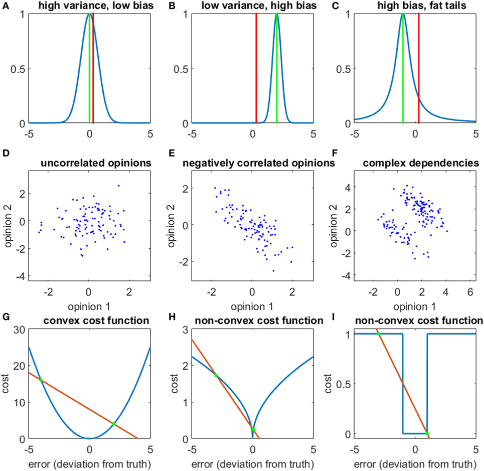
Figure 1. The three factors that influence aggregation rules. (A–C): the relationship between individual opinions and the truth. Blue curves show group opinion distributions, red lines mark the location of the truth, and green lines mark the average group opinion. (A) A low bias but high variance distribution. (B) A high bias, low variance distribution. (C) A biased distribution with fat tails marked by the slower decay of the probability distribution away from the mean. (D–F) The relationship between the opinions of two individuals. (D) Uncorrelated opinions. (E) Negatively correlated opinions. (F) A complex dependence between two individual’s opinions. (G–I) Various cost functions. (G) A convex cost function (see Section 5 and Appendix A1.1–1.2 for more extended discussions). (H,I) Two non-convex cost functions. In order to illustrate the property of convexity, we have also intersected each cost function with a red line. See section 5 for a further explanation.

Just like opinions carry information regarding the truth, they may also carry information about each other. As an everyday example, let us look at a group of school children who have been taught to eat or avoid certain types of mushrooms from a common textbook. Our scenario creates an interesting situation, where one need not poll the entire class to know what all kids think. Asking only a few students for their opinion on any particular mushroom will tell us what the others likely think. Their opinions are now generated through a shared underlying mechanism (Barkow et al., 1995) and may be said to have a mutual dependence.

Mutual dependencies between variables influence the optimal decision rule in many ways. Pairs of variables that show a mutual relation to each other are frequently studied using their correlations (though there are other forms of dependencies not captured by correlations). Correlations can impede the emergence of collective intelligence (Bang and Frith, 2017). Thus, in the social sciences, much effort has been devoted to methodologies aimed at eliminating correlations and encouraging independence (Janis, 1972; Myers and Lamm, 1976; Kahneman, 2011), but we will review situations where correlations boost group performance as well. Interestingly, while it is true that if we are using an optimal decision rule, then on average, more information can only improve our performance or leave it at the same level, this conclusion does not hold for suboptimal decision rules. In such cases, extra information can actually decrease the performance (see section 4). Therefore, correlations and dependencies within opinion pools are well worth studying. Figures 1D–F illustrates the diverse forms which inter-individual opinion dependencies may take.

After we have determined the relationship between the truth and our information sources as well as the information that the opinions provide about each other, we have all the necessary knowledge to calculate the probability distribution of the truth. Yet knowing the likely values of the truth alone will not be sufficient. Before we are able to produce a final estimate, we need to consider the cost of errors (Green and Swets, 1988). We need a mathematical rule specifying how much cost is incurred by all the various different deviations from the truth which may occur when we make an error. A more extended definition and discussion of cost functions will follow in section 5. At this point, the reader might gain a quick intuition into the topic by examining graphical illustrations of various cost functions in Figures 1G,H.

Cost functions are typically application dependent, but in academic papers, the most commonly used cost functions seem to be the mean squared error and the mean absolute deviation. The cost function has an important influence on the final decision rule. For example, if errors are penalized according to their absolute value, then an optimal expected outcome is achieved if we give as our answer the median of our probability distribution, whereas in the case of the squared error cost function, we should produce the mean of our probability distribution as final answer (Bishop, 2006). As the cost function changes, so changes our decision rule as well. It will turn out that certain cost functions will lead us away from averaging methodologies toward very different decision rules.

Throughout the review, we will make references to the aforementioned three concepts of statistical decision theory and how they have informed the design of new methods for knowledge aggregation. To help structure our review, we have grouped together methods into subsections according to which factor is most relevant for understanding the aggregation methods, but since ideally an aggregation procedure will make use of all three concepts, a strict separation has not been maintained and all concepts will be relevant to some degree in all subsequent chapters.

3. The Relationship Between Individual Opinions and the Truth

In decentralized systems, individual agents may possess valuable information about many different aspects of the environment. Ants or bees know the locations of most promising food sources, humans know facts of history, and robots know how to solve certain tasks. But the knowledge of individual agents is usually imperfect to some degree. For the purposes of decision-making and data aggregation, it is useful to have some kind of quantitative characterization of the knowledge of individual agents. Probability distributions and empirical histograms (Rudemo, 1982) are a convenient means to characterize the expected knowledge possessed by a randomly selected individual.

If the truth is known and we have a way to systematically elicit the opinions of random members in a population, then constructing opinion histograms is technically straightforward. Three key characteristics of the empirical histogram are known to be very important for data aggregation: the bias, the variance, and the shape of the distribution (Geman et al., 2008; Hong and Page, 2008). The bias measures the difference between the average group opinion and the truth. The smaller the bias, the more accurate is the group. The variance characterizes the spread of values within the group. If group member opinions have large variance, then we need to poll many people before we gain a good measure of the average group opinion (see Appendix A1.3 for formal mathematical definitions of above terms and Figures 1A–C for a pictorial explanation).

The shape of the distribution is a more complicated concept. Many empirical distributions do not have a shape that is easily characterized in words or compact algebraic expressions. If one is lucky enough to find a compact characterization of the distribution it can greatly improve the practical performance of wisdom of the crowd methods (Lorenz et al., 2011; Madirolas and de Polavieja, 2015). In the absence of an explicit description of the distribution, it is helpful to look at qualitative features such as the presence or absence of fat tails. Distributions with fat tails show strong deviations from the Gaussian distribution and are distinguished by unusually frequent observation of very large outliers (Taleb, 2013).

3.1. Leveraging Information about Biases and Shapes

Each of the abovementioned features of the empirical distribution can be leveraged to improve group intelligence. We begin with biases. Biases on individual questions are not very helpful per se. When those same biases reliably recur across questions, they become useful. The minds of humans and animals make systematic errors of estimation and decision-making which ultimately stem from our sensory and cognitive architecture (Tversky and Kahneman, 1974; Barkow et al., 1995). These biases can also affect crowd estimates (Simmons et al., 2011). Whalen made use of the concept of biases for improving crowd estimates of expected movie gross revenues (Whalen and Yeung, 2015). Whalen began by asking people to forecast the gross revenues of various movies. When he graphed crowd averages against the truth an orderly pattern became apparent. Crowds systematically underestimated the revenues of all movies. The bias even appeared greater for higher grossing movies. The remedy to the problem was straightforward—crowd estimates needed to be adjusted to higher values. The up-weighting procedure considerably increased crowd accuracy on a set of hold-out questions which were not used to estimate the bias.

Another important practical use case of biases concerns crowd forecasting of probability distributions. Humans systemically underestimate the probability of high probability events as well as overestimating the probability of low probability events (Kahneman and Tversky, 1979). Human crowd predictions show similar biases and a debiasing transformation can then be used to improve the accuracy of crowd probability predictions (Ungar et al., 2012). A related method uses opinion trimming to improve the calibration of probability forecasts (Jose et al., 2014).

Similar to the way knowledge about biases helps design better aggregation methods, knowledge about the shape of the distribution is critical for designing the best knowledge integration techniques. In many real datasets, varying expertise levels deform the distribution of opinions from a normal distribution to a fat-tailed distribution (Galton, 1907; Yaniv and Milyavsky, 2007; Lorenz et al., 2011). Fat-tailed distributions generate more frequent outliers that have large effects on estimating the mean when using classical statistical procedures. When data are generated from a fat-tailed process, it is better to use robust statistical estimation methods. A useful technique for estimating the mean involves leaving out a certain percentage of the most extreme observations (Rothenberg et al., 1964). Pruning away the outliers may improve wisdom of the crowd estimates (Yaniv and Milyavsky, 2007; Jose and Winkler, 2008). One particular type of distribution called the log-normal distribution even has a convenient estimator known as the geometric mean which can be very effective as an estimation procedure for datasets conforming to the distribution.

3.2. Individuality and Expertise

Previously, we treated all members of the crowd as identical information carriers. This is generally not the case. Sources of information may be distinguished from one another by their type, historical accuracy, or some other characteristic. When information is available regarding the reliability of sources, a weighted arithmetic mean typically works better than simple averaging (Silver, 2012; Budescu and Chen, 2015; Marshall et al., 2017). For example, sites aggregating independent polls produce their final predictions by weighting the independent polls proportionally to the number of participants in each poll, because, all other things being equal, larger polls are more reliable (Silver, 2012).

In the field of multi-agent intelligence, individuals are typically broadly similar, but may nevertheless have some individual characteristics. One particularly frequently explored topic concerns analysis of historical accuracy in order to improve future predictive power. Historical track records are, for example, used to form smaller but better informed subgroups. Having a subgroup rather than a single expert allows the averaging property to stabilize group estimates whilst avoiding the systematic biases which often plague amateur opinions. Mannes et al. (2014) have studied the performance of select crowds of experts on an extensive collection of 50 datasets. Experts were first ranked relative to past performance and subsequently, the future predictions of either the whole crowd, the best member of the crowd or a collection of the best 5 members of the crowd (the select crowd) were compared with each other. The select crowd method systematically outperformed other methods of knowledge aggregation.

In another study (Goldstein et al., 2014), nearly 100,000 thousand online fantasy football players were ranked in order of past performance. The investigators then formed virtual random subgroups which varied in size and the amount of experts they contained. The behavior of the subgroups was used to predict which players will perform best in English Premier League games. Analysis indicated that small groups of 10–100 top performers clearly out-competed larger crowds where expert influence was diluted, thus showing the benefits of taking expertise into account. In general, following the experts is expected to be beneficial if we have both good track records and there is a wide dispersion in individual competence levels, while for relatively uniform crowds averaging methods perform as well or better (Katsikopoulos and King, 2010).

When extensive historical records are missing, experimental manipulations have been invented to tease out the presence of expertise. One such strategy is known as the wisdom of the resistant (Madirolas and de Polavieja, 2015). Wisdom of the resistant exploits humans’ tendency to shift their opinion in response to social information if there is private uncertainty. The natural expectation is for people with more accurate information to have less private uncertainty and to be more resistant to social influence. Wisdom of the resistant methodology consists of a two-part procedure which takes advantage of this hypothesis about human microbehavior. In the protocol, people’s private opinions are elicited first and they are subsequently provided with social information in the form of a list of guesses or their mean from other participants to observe how subjects shift their opinion in response to new information. Subjects are ranked in order of increasing social responsiveness and a subgroup with the least flexible opinions is used to calculate a new estimate for the quantity of interest (the exact size of the subgroup is calculated using a p-value based statistical technique so as to still make as much use of the power of averaging as possible). In line with theoretical expectations, the new estimate often improves relative to the wisdom of the crowd (Madirolas and de Polavieja, 2015).

Interestingly, several popular models of decentralized collective movement and decision-making use rules which spontaneously allow the more socially intransigent individuals to have a disproportionately large effect on aggregate group decisions (Couzin et al., 2005; Becker et al., 2017). Natural collectives might, thus, implicitly make use of similar methodologies, although the computation implemented by local rules oriented algorithms is more context dependent (Couzin et al., 2011).

A methodology similar to wisdom of the resistant was recently proposed (Prelec et al., 2017), which asked subjects to predict both the correct answer and the answer given by the majority. The final group decision was produced by selecting an answer which proved surprisingly popular (more people chose this answer than was predicted by the crowd). Both methodologies leverage the presence of an informed subgroup in the collective and they provide means of identifying informed subgroups without historical track records.

Many of the problems where crowd wisdom is most needed concern areas where there are no known benchmarks or measures of ground truth against which expertise could be evaluated. Under such conditions, we can still determine individual expertise levels by as light reformulation of the problem. Instead of finding the answer to a single question, we again seek to answers to an ensemble of questions. For question ensembles, recent advances in machine learning can be brought to bear on the problem of jointly estimating which answers are correct and who among the crowd are likely to be the experts (Raykar et al., 2010).

As an example, consider the case of a crowd IQ test (Bachrach et al., 2012), where many people fill out the same IQ test in parallel. Here, a machine learning method known as a graphical model is applied to the problem of collective decision-making. The IQ test was an ensemble of 50 questions and IQ was linearly related to the number of correct answers given by the decision-maker (the IQ ranges measured on the test were from 60 to 140). Since individual IQ varies, we can characterize each person with the probability of correctly answering a randomly chosen question on the test, p. We cannot measure p directly, but since the average probability of a correct decision is 75% and the crowd majority will answer most questions correctly most of the time, then we can get an estimate of p by looking at how well each persons answers correlate with the majority vote. These estimated p values can subsequently be used to refine our estimates of which answers are correct, which in turn can be used to refine our estimated p values further. Stepping through this iteration multiple times allows the algorithm to improve on the results of the majority vote.

In the case of crowd IQ, a majority vote among 15 participants produces an average crowd IQ of approximately 115 points, while the machine learning algorithm can be used to boost this performance by a further 2–3 points. It is also interesting to see that unlike what would be expected from Condorcet, crowd IQ effectively plateaus after a group size of 30 is reached. A crowd of 100 individuals has a joint IQ score of merely 120. Given that a group of 100 individuals is very likely to contain a few people with near-genius level (>135) IQ, the study also illustrates why it could sometimes be well worth the effort to find an actual expert rather than relying on the crowd.

Is it possible to utilize expertise if we poll the crowd on a single question rather than on an ensemble? Empirical studies thus far seem to be lacking. We have built a scenario that shows the possibility of improving on the majority vote under some special conditions.

Consider again a crowd of people choosing among some options, where a fraction 1 − k will choose their answer randomly, while a fraction of k experts know the correct answer. During actual voting, we sample randomly N individuals from our very large crowd and let them vote. If our crowd members face a choice between two alternatives, then a random member of the crowd will be correct with probability $p=k+\frac{1}{2}\left(1-k\right)$, and Condorcet theorem will exactly describe how the crowd performance varies as a function of N and p. Suppose we now expand the two-way choice between the correct and incorrect alternative into an K-way choice between the two original choices and K − 2 irrelevant distractions. The final opinion is now chosen via a majority vote between the two relevant alternatives while ignoring all opinions landing on the distractions. In the appendix, we prove why the performance of our method for K > 2 is always strictly better than the performance of traditional majority voting where the crowd chooses only between 2 alternatives. As is apparent in Figure 2, the improvements in performance are quite dramatic, particularly for larger values of K and N. For very large values of K, the performance of the method tends to the same formula as the many-eyes model discussed in the next section (see Appendix A3 for proof).

FIGURE 2

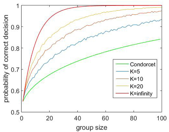
Figure 2. Using irrelevant alternatives to improve group performance- a simulation study. Group performance curves (calculated from a computer simulation) as a function of the number of total alternatives K using our new voting procedure. The percentage of experts in the crowd is fixed at 10% for this plot. The different colors of curves illustrate how varying the group size N influences group performance for a fixed K. The green curve gives a comparison with Condorcet theorem (which is technically equivalent to the case N = 2). See Appendix A3 for proof of why performance always exceeds the Condorcet scenario.

The efficacy of this hypothetical procedure depends on how closely our assumptions of human micro behavior match with our model. This example merely illustrates that scenarios might be constructed and empirically tested for specific problems which allow investigators to significantly improve performance relative to the Condorcet procedure. Perhaps the closest practical analog to this idea is the use of trap questions in crowd sourcing to filter out people who are insufficiently attentive to their task (Eickhoff and De Vries, 2011).

4. The Role of Dependencies

Before we dive into the most catastrophic failures of averaging, it is instructive to once more consider why averaging sometimes works very well. As described above, the majority vote was first analyzed in 18th century France, where Marquis de Condorcet proved his famous theorem demonstrating the efficiency of majority voting for groups composed of independent members (see Appendix A1.4 for a mathematical description of Condorcet voting). A crucial tenet underlying his theorem concerns the assumption of independence (Condorcet, 1785; Boland, 1989; Sumpter, 2010). Condorcet theorem requires more than just a group of individuals who do not interact or influence each other in a social way. It requires the jury members to be statistically independent. In a group with statistically independent members, the vote of any member on a particular issue does not carry any information about how other members of the group voted. For the particular case of Condorcet, if an individual has an expected probability p of producing the correct answer, then we do not need to modify our estimate of the value of p after we learn whether his partner voted correctly or incorrectly.

In all the examples covered in the current section, the aforementioned statistical independence property no longer holds and learning any individual’s opinion now also requires us to modify our estimate of his partners’ opinions. The lack of statistical independence is not just a feature of our examples. Statistical independence is difficult to guarantee in a species where most individuals have a partially shared cultural background and all members have a shared evolutionary background which constrains how our senses and minds function (Barkow et al., 1995). Because of that shared background, the opinions of non-interacting people are also likely to be correlated in complex ways.

It is easy to notice some ways in which correlations retard collective intelligence. Using the abovementioned example of school children who all learned about mushrooms from a common textbook, we can conclude that in such a scenario, the group essentially behaves as a single person and no independent cancelation of errors takes place (Bang and Frith, 2017). But the influence of opinion dependencies is sometimes even more destructive. We can imagine a group composed of a very large number of members who need to answer a series of questions. On any random question, the probability of receiving a correct answer from a randomly chosen group member is p. Similar to Kuncheva et al. (2003), we can ask what is the worst possible performance of a group with such properties. In the worst-case scenario, questions come in two varieties: easy questions, where all group members know the correct answer, and hard questions, where infinitesimally less than 50% of the people know the correct answer. On the easy questions, the majority vote will lead to a correct answer, while on the hard questions, the majority vote will lead to incorrect decisions. Intuitively, the 50–50 split on the hard questions will ensure that the greatest possible number of correct votes will go to waste since for those questions the correct individual votes do not actually help the group’s performance. With such a split of votes, the group will perform as poorly as possible for a given individual level performance (see Kuncheva et al. (2003) for more details). In order for the average person to have an accuracy of p, the proportion of hard questions (t) must satisfy $p=\frac{1}{2}\left(1-t\right)+t$ which means that the group as a whole will be correct in only 2p − 1 fraction of cases. The result is quite surprising—a group where the average individual is correct 75% of the times may as a whole be correct in only 50% of the questions.

Dependencies, however, are not necessarily detrimental to performance. As we explain in the following two subsections, whether or not correlations and dependencies help or hurt performance depends on the problem at hand (Averbeck et al., 2006; Davis-Stober et al., 2014) and, crucially, on the decision rule used to process the available data. These general conclusions extend to the domain of collective decision-making as well.

4.1. Correlations Can Improve Performance in Voting Models

We begin our discussion of alternative voting procedures with the important example of collective threat detection. Here, the majority vote is eschewed in favor of a different decision rule. A single escape response in a school of fish (Rosenthal et al., 2015) or some-one yelling fire in a crowded room can transition the whole collective into an escape response. A collective escape response begins even though the senses of a vast majority detect nothing wrong with their surroundings. The ability of an individual to trigger a panic is treated very seriously. In the US legal system, one of the few instructions which restricts freedom of speech concerns the prohibition against falsely yelling fire in a crowded room.

Despite the slightly negative connotation of the word, panics are a useful and adaptive phenomenon. For example, panics help herding animals avoid predators after collective detection of a predator (Boland, 2003). Improved collective predator detection and evasion is known as the many-eyes hypothesis and it is thought to be one of the main drivers behind the evolution of cooperative group behavior (Roberts, 1996).

Why is it rational to ignore the many in favor of the few? Consider a very simple probabilistic model to explain this behavior. Let us think of a single agent as a probabilistic detector. Let us also assume that the probability of the agent detecting a predator where none is present is zero, in other words, there are no false alarms. The probability of an animal detecting a predator when one is in fact present is t. The value of t might be much less than one, because detecting an approaching predator is hard unless you happen to catch it in motion or look directly at it. Under the conditions of our scenario, it is clear that other animals will begin an escape only if a predator is in fact present. It follows that if others are escaping, you should begin an escape as well.

For the sake of giving a concrete example (a formal mathematical treatment and derivation of all the formulas related to the panic models which follow are found in the Appendix), let us analyze the case where the probability of a predator attacking is 50 h case makes up 50% of the total incidents. For t = 0.4, it gives a value of p = 0.7 (Figure 3, value at group size = 1). For group sizes larger than 1, the majority vote performs worse than this value because if a predator is indeed attacking, only a minority of the animals will detect the predator and the majority votes that there is no predator present (Figure 3, black line). The majority of a large group is then only correct in the 50% of the cases in which there is no attack (Figure 3, black curve for large groups).

FIGURE 3

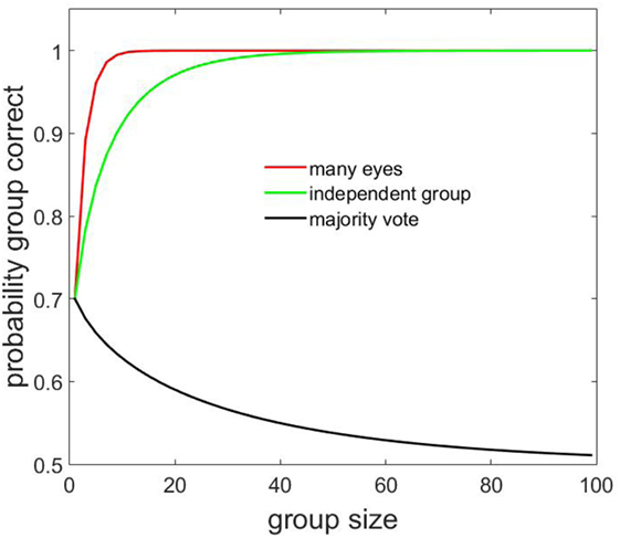
Figure 3. Following the informed minority vs. majority voting. The red curve plots the percent of correct threat assessment as a function of group size for the optimal detection (many eyes) model, where even detection by a single individual can trigger a collective response. The black curve illustrates how performance would change with group size if animals used the majority vote. The green curve plots the performance of a crowd of independent individuals with same individual competence as for the many-eyes model. See main text for details and Appendix A2 for the mathematical derivation of the three lines.

In real collectives, the majority vote is rejected as a decision rule, and even a single detection by a single member is enough to alert the whole group to the danger. Under such a strategy, the probability of a group correctly detecting a predator increases very rapidly as the group size N increases as 1 − 0.5(1 − t)^N (Figure 3, red curve; see Ward et al. (2011) for use of the same expression, known as many-eyes model). The group then detects a predator much more efficiently than if it was relying on the majority.

What would the performance of the group be like if the animals were all statistically independent from each other while retaining the same average individual performance as in the many-eyes model. Now, instead of analyzing the majority decision for the no attack and attack cases separately, we simply plug the probability p = 0.7 into the Condorcet majority formula (Figure 3, green curve). The plot clearly shows the superiority of the many-eyes model over the independent group. Inter-animal dependencies have increased group intelligence.

The idea of harnessing correlations to increase group performance appears rarely discussed in the voting literature. For example, a recent comprehensive review of group decision-making and cognitive biases in humans had an extensive discussion of how inter-individual correlations can hurt group performance and the ways in which encouraging diversity helps overcome some of the problems (Bang and Frith, 2017). Yet the positive side of correlations and how they may help performance was not covered. Likewise, in another paper on fish decision-making, quorum decision rules were compared against Condorcet’s rule as if it was the optimal possible decision rule (Sumpter et al., 2008), even though other rules which account for potential correlations are capable of producing better group performance.

It is also important to note that in the case of applying the majority vote to estimate the presence of a threat, none of the reasons usually provided to explain away the failures of the majority vote apply (Surowiecki, 2004; Kahneman, 2011; Bang and Frith, 2017). The initial votes could be cast completely independently (without social interaction) and each new vote could add diverse and valuable new information to the pool of knowledge and yet the majority vote would still fail. The insight here is that the majority vote is inappropriate because it does not match with the distribution of knowledge across the collective: a minority has the relevant information about the presence of a predator.

If we examine Figure 3 more carefully, we see a region corresponding to large group sizes (N > 45), where the majority vote for the independent group and the panic model both give near-perfect performance (though the panic model always strictly outperforms the independence model for all N > 1, see Appendix A3 for proof). It is, therefore, natural to wonder whether encouraging independence might be a useful practical rule of thumb if one is sure to be dealing with very large groups.

The independence-focused line of reasoning runs into difficulty when one considers the costs necessary to make animals in the group perfectly independent. To guarantee statistical independence, it is not sufficient to merely make the animals in our group weakly interacting. The correlations originate because all animals experience threat or safety simultaneously. Correlations only disappear when the probability of any individual making a mistake is equal in both the threat and the no threat scenario. Any time, the above condition fails to hold, correlations appear, which makes it clear why establishing perfect independence is a precarious task likely to fail in the complexity of the real world. By contrast, the panic model is a robust decision rule, stable against variations in probabilities and guaranteed to give a better than independent performance for small group sizes. It, thus, becomes more apparent why natural systems have preferred to adapt to and even encourage correlations rather than fight to establish independence.

We note that even for the many-eyes model, in practice there is usually a small probability of a false alarm, and field evidence from ornithology demonstrates how animals can compensate against rising false alarm rates by raising the threshold for the minimum number of responding individuals necessary to trigger a panic (Lima, 1995). We point the interested reader to Appendix A2 for a mathematical treatment of the false alarm scenario.

The decision rule adopted by vigilant prey could be called a “full vote.” In order to declare a situation safe, all individuals must agree with the proposition. A similar rule has been rediscovered in medical diagnostics. In medical diagnostics, some symptoms such as chest pain are inherently ambiguous. Sudden chest pain could signal quite a few possible conditions such as a heart attack, acid reflux, a panic attack, or indigestion. In order to declare a patient healthy, she must pass under the care of a cardiologist, a gastro-enterologist, and a mental health professional. All experts must declare a patient healthy before he can be released from an examination. In the case of a panel of experts, their non-overlapping domains of expertise help insure the effectiveness of the full vote.

A similar idea has been implemented in the context of using artificial neural networks (a machine learning method, see Section 6 for more details) to detect lung cancer in images of histological sections (Zhou et al., 2002). An ensemble of detectors is trained using a modified cost function which heavily penalizes individual neural networks when they declare a section falsely malignant. The training procedure makes false alarms rare, so the full vote procedure can be used to detect cancer more efficiently than if the networks had been stimulated to be maximally independent.

4.2. Correlations and Continuous Variables

In the case of averaging opinions about a continuous quantity, correlations also have a profound effect on group performance. The average error on a continuous averaging task is given by the sum of the bias and the variance (Hong and Page, 2008). Variance declines as we average the opinions of progressively larger pools of opinions (Mannes, 2009). Correlations control how rapidly the variance diminishes with group size. The speed of decrease is slowest when correlations are positive. Finding conditions where errors are independent helps speed up the decrease of variance. The most rapid decrease occurs when correlations are negative (Davis-Stober et al., 2014). For large negative correlations, the errors in pairs of individuals almost exactly cancel and even a very small group can function as well as a large crowd of independent individuals. The benefits of negative correlations are exploited in a machine learning technique termed negative correlation learning (Liu and Yao, 1999).

Correlations can be leveraged most efficiently when we have individual historical data. Personalized historical records enable the researcher to estimate separate correlation coefficients for every pair and compute the optimal weighting for every individual opinion. The benefits of correlation-based weighting are routinely applied in neural decoding procedures, where the crowd is composed of groups neurons and opinions are replaced by measurements of neural activity. Averbeck et al. (2006), for example, study the errors induced in decoding if neural activity correlations are ignored, and find that ignoring correlations generally decreases the performance of decoders when compared to the optimal decoder which takes the information present in correlations into account. Similar to Davis-Stober et al. (2014) who study correlated opinions, they find a range of situations where correlations improve decoding accuracy as compared to independently activating neurons.

5. The Role of Cost Functions

5.1. Measures of Intelligence

Collective intelligence is of course a partly empirical subject. After the theoretical work of Condorcet, the next seminal work in the academic history of wisdom of crowds comes from Galton, whose work we briefly described in the introduction. The conclusion of his study was that simple averaging of individual estimates is, as an empirical matter, a more useful way to estimate quantities than relying on faulty individual opinions. In addition to Galton’s work, another classic study of crowd intelligence involved subjects estimating the number of jelly beans or marbles contained in a jar (Treynor, 1987; Krause et al., 2011; King et al., 2012). The true number of beans is typically between 500 and 1,000, so exact counting is not feasible for the subjects. If the crowd is larger than 50 individuals, the crowd median and/or mean opinion typically comes within a few percent of the true value. The effect is even somewhat independent of the sensory modality involved. In a study of somatosensory perception, 56 children estimated the temperature of their class room. The average of their 56 guesses deviated from the true value by just 0.4°(Lorge et al., 1958).

Galton and many others who followed gave empirical demonstrations regarding the remarkable effectiveness of simple averaging without any mathematical arguments as to why the phenomenon occurs. Perhaps because the performance of the crowd in these early studies was spectacularly good, there was also a lack of explicit comparison to other ways of making decisions. In more recent years, there has been more focus on the failure of crowds. Many examples are known where crowds fail to come close to the truth (Lorenz et al., 2011; Simmons et al., 2011; Whalen and Yeung, 2015). Lorenz et al. (2011) report an average crowd error of nearly 60% (relative to the truth) in a set of tasks consisting of estimating various geographical and demographic facts. In psychology, there is a rich literature on the heuristics and biases utilized in human decision-making (Tversky and Kahneman, 1974), which can also bias crowd estimates (Simmons et al., 2011).

Examining collective performance in cases where the crowd makes practically significant mistakes led to a need to perform more explicit comparisons between different methodologies. It is common to compare wisdom of crowd estimates with the choosing strategy.

In the choosing strategy, we pick one opinion from the crowd at random and use that opinion as our final estimate. To quantitatively compare averaging and choosing, we first measure the error of a guess as error = |our guess − true value|, where |x| stands for absolute value of any number x. To assess the impact of an error, we also have to specify a cost function. A cost function is a mathematical measure which specifies how damaging an error is to overall performance. The smaller the overall cost, the better the performance. Common cost functions found in the literature are the absolute error (also called the mean absolute deviation) and the squared error cost functions. If we are using the choosing strategy, then the error will typically be highly variable from person to person, because individual guesses are variable. In order to compare the performance of the choosing strategy with the performance of the crowd average opinion, we average the costs of individual guesses and then compare the average cost with the cost of the mean crowd opinion.

We illustrate the role of a cost function with a numerical example. In an imaginary poll, we query four people about the height of a person whose true height is 180 cm. The group provides four estimates: 178, 180, 182, and 192 cm. The corresponding error values are |178 − 180| = 2, |180 − 180| = 0, |182 − 180| = 2, and |192 − 180| = 12. The mean absolute deviation cost is (2 + 0 + 2 + 12)/4 = 4. Since the crowd mean is 183, the crowd opinion induces a cost of 3 only. In this example, averaging outperformed choosing. Similarly, for the squared error cost function, the choosing strategy has an expected error of (2² + 0² + 2² + 12²)/4 = 37, while the crowd mean causes an error of (183 − 180)² = 9. The crowd mean again outperforms random choice.

It has become common practice to emphasize the superiority of wisdom of crowd estimates over the choosing strategy with performance measured through use of the mean absolute deviation or the mean squared error cost function (Hong and Page, 2008; Soll and Larrick, 2009; Manski, 2016). An unconscious reason behind the popularity of the comparison might be that it will always yield a result that casts collective wisdom in a favorable light. A mathematical theorem known as Jensen’s inequality guarantees the superiority of the average over the choosing strategy for all convex cost functions. The mean squared error and the mean absolute deviation are both examples of convex cost functions.

The exact definition of a convex function is rather technical (see Appendix A1.1–1.2 for a formal definition of both convexity and Jensen’s inequality), but we may gain some intuition into the concept if we examine what happens if we intersect various cost functions in Figures 1G–I with randomly drawn lines. For each panel, if we focus on the relationship between the red line and the blue curve in between the green dots, we see that for panel G the red line is always above the blue curve, whereas for H and I, the red line may be either above or below the blue line depending on which region between the green dots we focus on. In fact, for function G, the blue curve is always below the red line for any possible red line we may think of as long as we focus on the region that is between the two points where the particular line and the curve intersect. It is this property that makes G a convex function and allows us to guarantee that the group average error is always smaller than the average individual error.

Some authors have elevated Jensen’s inequality and similar mathematical theorems to the status of a principle which justifies the effectiveness of collective intelligence (Surowiecki, 2004; Larrick and Soll, 2006; Hong and Page, 2008). We hold ourselves closer to the position of authors who have questioned these and similar conclusions (Manski, 2016). Fundamentally, Jensen’s inequality is merely a property of functions and numbers. We might sample 100 random numbers from a computer and use them to estimate the year Winston Churchill died. If I measure my performance using convex cost functions, then the average of my sample will induce a lower cost than a choosing strategy. Should I say that the collection of random numbers possesses collective intelligence?

Furthermore, reporting collective performance on a single question using a single numerical measure exposes the investigators to an unconscious threat of cherry-picking. Perhaps the good performance of the crowd was simply an accidental coinciding of the crowd opinion with the true value of one of the many possible questions that many investigators have proposed to crowds over the years.

Instead, we advocate the study of correlations on ensembles of questions as was recently also done by Whalen and Yeung (2015). We illustrate the procedure by reanalysis of a dataset from the study by Yaniv and Milyavsky (2007), where students were asked to estimate various historical dates. On Figure 4, we have plotted the true values versus the wisdom of crowd estimates for 24 questions. Such an analysis gives a good visual overview of the data. For example, it is immediately clear from the plot that wisdom of crowd estimates are strongly correlated with the truth across the ensemble and there is clearly knowledge present in the collective. We find that on an average question, the crowd wisdom missed the truth by nearly 30 years. On certain questions, the crowd error was undetectable, while on others the crowd was off by nearly 100 years. Overall, the collective performance is of mixed quality, with excellent performance on some questions, mediocre performance on others, and no clear systematic biases.

FIGURE 4

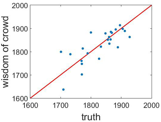
Figure 4. Wisdom of the crowd for historical dates. Mean of 50 independent opinions versus true values for 24 questions concerning historical dates. The red line marks the ideal performance curve; real performance frequently strongly deviates from that line. Data from Yaniv and Milyavsky (2007).

5.2. Beyond Convexity

Aside from the fact that Jensen’s inequality may be applied to any collection of numbers, there is another problem with analysis of collective performance as they are currently commonly carried out. There is an exclusive focus on convex cost functions. Yet many real-world cost functions are non-convex. In a history test, problems will typically have only a single acceptable answer. A person who believes the US became independent in 1770 will receive zero points for his reply, just like a person who believes the event took place in 1764, even though the first person was twice as close to the truth. Similarly, an egg which was cooked for 40 min too long is not substantially better than an egg over-cooked for 120 min as both are inedible and should induce similar costs for the cook.

What happens to the performances of the averaging and the choosing strategies when we change our cost from a convex to a non-convex function? We will once again make use of our aforementioned example of guessing heights. As our new cost function, we will use a rule which gives a penalty one to all examples that deviate from the truth by more than 1 cm and assigns a cost of 0 to answers which are less than 1 cm away from the truth. Our set of opinions was 178, 180, 182, and 192 cm with the true value lying at 180 cm. In this case, the crowd mean has a penalty of 1, because the crowd mean of 183 misses the true value of 180 by more than 1. Three out of four individual guesses also miss the truth by more than a year, but one guess hits the truth exactly, so the average cost of the choosing strategy is (1 + 0 + 1 + 1)/4 = 0.75. In this case, the crowd mean underperforms relative to the choosing strategy. A similar effect results from using a cost function which penalizes guesses according to the square-root of their absolute error. The square-root cost function penalizes larger errors more than smaller errors, but the penalty grows progressively more slowly as errors increase. The crowd mean has a cost of $\sqrt{183-180}=1.7$. The choosing strategy has an expected cost of $\left(\sqrt{2}+\sqrt{0}+\sqrt{2}+\sqrt{12}\right)∕4=1.6$. The crowd mean incurred a higher expected cost than a randomly chosen opinion. Our examples illustrate that the best strategy for opinion aggregation is highly dependent on the cost function.

A different way to visualize the same result would be to consider the cost incurred by the same pool of opinions as the location of the truth varies. In Figure 5, we consider the cost performance of a fixed pool of 5 opinions (with values −1, −0.5, 0, 0.5, and 1) as a function of the location of the true value. As can be seen from the graph, convex cost functions such as the mean square error and the mean absolute deviation produce a lower error when the mean opinion is used independently of where the true value is located. Non-convex functions such as the mean square root of the absolute deviation reveal a more complex picture. Sometimes it is better to choose and sometimes it is better to average. No simple optimal prescription is possible.

FIGURE 5

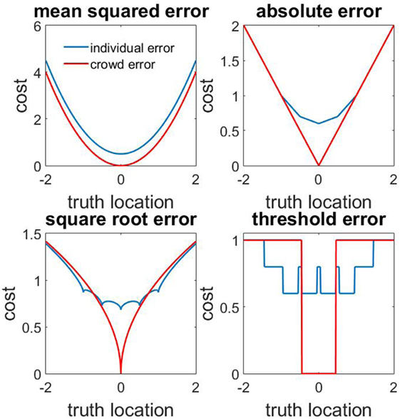
Figure 5. Comparison of averaging and choosing strategies for different cost functions. Cost incurred by the averaging strategy (red curve) and the choosing strategy (blue curve) as a function of the location of the true value for four different cost functions. The five opinion values on which the performance is calculated: −1, −0.5, 0, 0.5, and 1. Quadratic cost is strictly convex, and mean (red) is then always below choosing (blue). Absolute error cost function is weakly convex, and mean (red) is then always below or equal to choosing (blue). Square the third and fourth curves are neither convex nor concave. The threshold cost function gives a cost of 0 if an opinion is closer than 0.45 to the truth and a cost of 1 for all other values.

If the cost function is not convex, then Jensen’s inequality no longer applies and averaging is not guaranteed to outperform choosing. As our last two examples showed, the opposite might be the case. In that light, it is intriguing to note that when humans take advice from other people, they often opt for a choosing strategy rather than an averaging strategy (Soll and Larrick, 2009). This behavior has been seen as suboptimal (Yaniv, 2004; Mannes, 2009; Soll and Larrick, 2009), but it may in fact be a rather rational behavior. The human crowd often contains a substantial fraction of experts who know the answers to certain questions while other members of the crowd have less information about the question at hand. If we assume that advice becomes beneficial only if it reaches relatively close to the truth, then it becomes rational to pick a random opinion in the hopes of hitting expert advice, rather than relying on the crowd mean, which might lie far from the truth because of distortions by non-expert advice.

To analyze the problem more systematically, we have re-examined an experiment from Yaniv and Milyavsky (2007), where 150 students were individually presented with questions about when 24 prominent historical events took place. They were subsequently provided with advice from two, four, or eight other students. The students had the option of combining their initial private opinion with further advice (the advice was anonymous and was not presented in person) from other subjects. They had financial incentives to provide maximally accurate answers in both the individual and the advice-taking part of the experiment. We found that after receiving anonymous advice, in approximately 70% of cases, subjects stayed with their initial private opinion or chose the opinion of one particular adviser as their final answer. In Figure 6, we plot the cumulative distribution of errors of the students initial private estimates (red) and their revised opinions after hearing advice (blue) from 2 (left), 4 (middle), or 8 advisers (right). These may be compared against a strategy of averaging the student opinion and all the advisory opinions received (Figure 6, black). The distribution of errors indicates that students adopt a strategy that produces a more frequent occurrence of low error answers than the averaging strategy (though, of course, as guaranteed by Jensen’s inequality, the mean absolute error of the averaging strategy is lower than the choosing strategy and the strategy adopted by the student population as a whole. The aggregate gains of averaging with respect to squared errors mainly originate from the reduced occurrence of extreme errors in the averaging strategy).

FIGURE 6

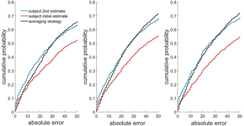
Figure 6. Errors in human advice-taking strategy compared to the averaging strategy. The cumulative distribution of errors of three advice-taking strategies for 2, 4, and 8 advisers. Red curve: initial subject opinion. Blue curve: subject opinions after hearing advice from 2 (left), 4 (middle), or 8 (right) randomly chosen fellows. Black curve: averaging strategy, which calculates a final estimate mechanically by averaging a subjects initial opinion together with all advisers opinions. Data from Yaniv and Milyavsky (2007).

It has been argued that durable real-world systems should evolve to a point where costs must be concave in the region of large errors as a robust design against large outliers (Taleb, 2013). It is interesting to speculate that human advice-taking diverges from the averaging strategy precisely because it takes advantage of non-convexity. So far, advice taking on everyday tasks has been understudied, possibly due to methodological difficulties. In the future, it will be illuminating to compare performance of choosing and averaging strategies on more naturalistic problems.

6. Embracing Complexity: A Machine Learning Approach

Previous research has primarily emphasized how simple rules of opinion aggregation can often produce remarkable gains in accuracy on collective estimation tasks. Yet we have also shown that such simple rules may fail in unexpected ways. We have outlined many possible sources of failure, which tend to occur if any of the following conditions are true:

1. The cost function is not convex.

2. The distribution of knowledge within the collective is inhomogeneous.

3. The pool of crowd opinions is not composed of statistically independent estimates.

4. The distribution of opinions has fat tails.

5. The crowd has significant and systematic biases.

One way to deal with these pitfalls is to use domain knowledge to design new estimation heuristics to compensate for the deficiencies in simpler methods. This approach has been successful and we have given several examples of their utility in practical applications. But these new heuristics often lack the mechanical simplicity of the averaging prescription and risk lacking robustness against unaccounted factors of variation in crowd characteristics.

It is the issue of unaccounted characteristics which should be most troubling to the theoreticians. It is easy to perform mathematical analysis of simple models such as Condorcet voting, but as we have previously shown, the confidence derived from such theoretical guarantees has a false allure. Usually, we do not have complete knowledge of all the complex statistical dependencies that occur in the real world and, therefore, the behavior of simple decision rules is liable to unpredictable in practice. The issue of practical unpredictability motivates us to examine ways to create collective intelligence in a way that makes more direct contact with the idea of optimizing real-world performance.

An appealing way to deal with greater complexity is to rely more on methodologies that incorporate complexity into their foundations. Machine learning is capable of learning decision aggregation rules directly from data and can be used to design computational heuristics in a data-driven manner. It can be used to either verify the optimality or near-optimality of known heuristics on a given task or to design new aggregation methods from scratch. While machine learning methods may on occasion be less intuitive for the user, they come with performance guarantees because they are inherently developed by optimizing performance on real-world data. The black box nature is a necessary price which one must pay for the ability to deal with arbitrarily complex dependencies.

Neural networks are one class of machine learning methods that allow the aforementioned procedure to be carried out automatically (LeCun et al., 2015). A neural network is composed of artificial neuron-like elements that transform input opinions into an output estimate. If the researcher has access to a dataset where the true value of the estimated quantity as well as the pool of crowd opinions are known for many groups, then it is possible to find a very close approximation of the optimal decision rule that brings the input opinions into desired outputs.

We will next illustrate the application of neural network-based methods for a simulated dataset, where we find the optimal decision rule in a data-driven manner, and we also apply the method to a cancer dataset where we show that a network has a better performance than the majority vote and previously proposed heuristics.

In our hypothetical example, we consider a group of 30 people that have repeatedly answered questions about historical dates. In our simulated crowd, 50% of individuals will know the answer approximately (their opinion will have a SD of ±0.1 around the true value). The other 50% are less informed and present a bias to lower values (mean bias −1 ± 0.2). Under this scenario, it is intuitively clear that an optimal decision rule would look for clusters within the pool of opinions and the network must also learn to ignore the opinions coming from the lower cluster. We examined whether a neural network would be able to learn a similar decision rule entirely from data. For our scenario, the crowd mean strategy had an average error of 0.50 whereas a neural network trained on opinion groups was able to reduce the average error to 0.04 (see Appendix A4 for details on training and network architecture), thus demonstrating that neural networks can learn useful approximations to reduce the average error.

We have also examined whether neural networks could improve upon the performance of previously proposed heuristics on a skin cancer classification dataset (Kurvers et al., 2016). In the dataset, forty doctors had given their estimations and subjective confidence scores (four point scale) on whether particular patients had malignant melanoma by examining images of their skin lesions. As in Kurvers et al. (2016), we used Youden’s index as a measure of accuracy, given by J = sensitivity + specificity − 1, with sensitivity defined as the proportion of positive cases correctly evaluated and specificity defined as the proportion of negative cases correctly evaluated. This measure weights equally sensitivity and specificity and it is, thus, insensitive to the unbalances of a dataset (in this case, more cases without cancer than with cancer). We then generated virtual groups of doctors and examined the accuracy of their aggregated judgments. If all doctors in the group agreed on a diagnosis, their joint shared opinion was used as the diagnosis. If there was disagreement, we compared the performance of the following three heuristics for conflict resolution:

1. Use the opinion of the more accurate doctor in the group (“best”).

2. Use the opinion of the more confident doctor (“confident”).

3. Use the opinion held by the majority (“majority”).

In the “best” and “confident” heuristics, if the higher accuracy or confidence was shared by more than one doctor, the majority opinion within that subgroup was selected. If in spite of all the selection rules, there still was a tie, 0.5 was added to the count of correct answers and 0.5 to the mistakes.

We also fitted a neural network that was given as input the historical accuracies of the doctors, their diagnosis on each case, and their declared confidence scores. For any input, the output of the network gave the probability of the given input being consistent with a cancer diagnosis. If the probability exceeded 50%, then the network output was counted as giving a cancer diagnosis. We asked whether a network can find an aggregation decision rule better than the heuristics. The network (a multilayer perceptron) trained with backpropagation on 50% of the data. Another 25% of the data were used as validation dataset. To minimize overfitting, we used the early stopping procedure, where the weights of our network are saved during every epoch of training and in our final testing, we use the version of the weights which gave highest performance on the validation dataset. Testing of the network was done in the remaining 25% of the dataset. Figure 7A gives the learning curve of one network on the test dataset depending on the number of training epochs. As an example, for groups of five doctors, we found mean network performance of J = 0.804 and SD of 0.060. The different heuristics had the following performance for the same data: 0.757 ± 0.060 (“best”), 0.767 ± 0.067 (“confident”), and 0.801 ± 0.061 (“majority”); see Figure 7B for mean improvement of network over heuristics.

FIGURE 7

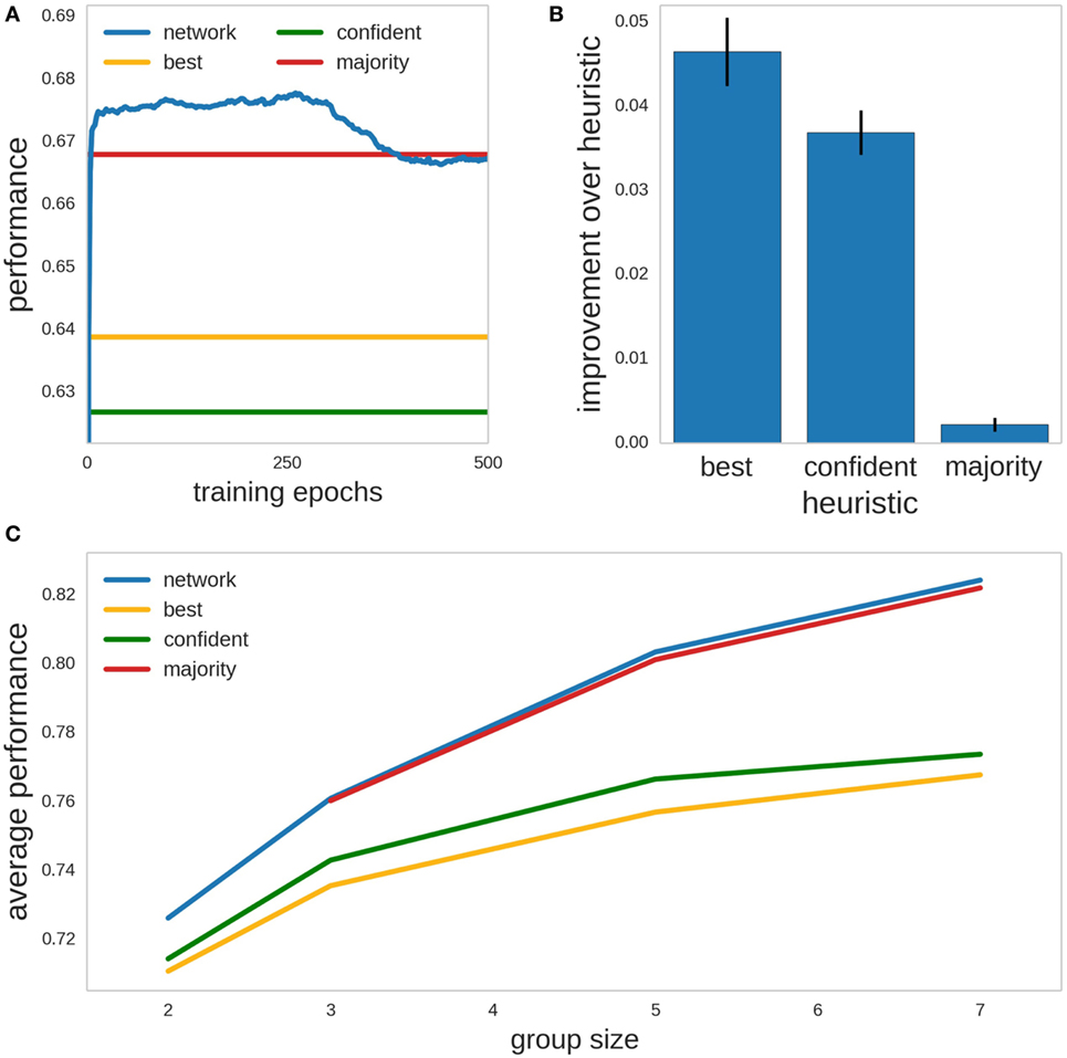
Figure 7. Network learning how to combine the opinions and confidence scores of three doctors into a cancer/no cancer classification rule. (A) Example of the training of one network for a particular partition of the data into 50% for training and 25% each for validation and test, for groups of 5 doctors. Shown is the evolution of the performance for the test data (Youden’s index, J = sensitivity + specificity − 1) of the network (blue line), and the performance of the best doctor heuristic (yellow line), the more confident heuristic (green line), and the majority heuristic (red line). (B) Mean improvement in Youden’s index of the network over the heuristics for groups of 5 doctors. Error bars are SEM. (C) Average performance of network and heuristics over all the validation sets, for groups of 2, 3, 5, and 7 doctors. Colors as in panel (A).

For groups of 2, 3, 5, and 7 doctors, we trained 50 networks using different 50 − 25 − 25% partitions of the data into training, validation, and test. We found that both the network and the three heuristics proposed improved their performance over the test cases for increasing group sizes (Figure 7C). The networks not only were more accurate than the rest of the heuristics for every group size (except against the majority voting for groups of 3 doctors) but also consistently better in every single partition of the cases into training, validation, and test (“best” and “confident”: p < 10⁻⁵ for all group sizes; “majority”: p = 0.0098, 0.027 for n = 5, 7. Wilcoxon signed-rank test). Overall, the difference between the optimal decision rule found by the network and the majority rule is small in this dataset and another way to view the results would be to say that the analysis through use of neural networks gives the user confidence that the majority rule is near-optimal for the present dataset. Note that we were unable to extend our analysis above the case of n = 7, because the permutation procedure we used to create pseudo-groups contains progressively greater overlaps for higher n since we are sampling from a limited pool of 40 doctors, and the statistical independence of our pseudo-groups is no longer guaranteed for larger n, which prevents reliable calculation of p-values.

7. Discussion

The collection of methodologies grouped under the umbrella term wisdom of crowds (WOC) has found widespread application and continues to generate new research at a considerable pace. As the number of real-world domains where WOC methods have been applied increases, researchers are beginning to appreciate that each new domain requires considerable tuning of older methods in order to reach optimal performance. Early focus on universal simple strategies (Condorcet, 1785; Surowiecki, 2004; Hastie and Kameda, 2005) has been replaced with a plethora of methods that have sought to find a better match between the problem and the solution and by doing so have shown increases in performance relative to the averaging baseline (Goldstein et al., 2014; Budescu and Chen, 2015; Madirolas and de Polavieja, 2015; Whalen and Yeung, 2015).

Many new avenues of research remain to be explored. Machine learning tools and improved ability to gather data provides the opportunity to learn more sophisticated WOC methods in a data-driven fashion (Rokach, 2010; Bachrach et al., 2012; Polikar, 2012; Sun et al., 2017). We are likely to learn much more about effective strategies of opinion aggregation through their widespread adoption. It will also be important to explore whether machine learning rules can be made intelligible to the end user. Techniques such as grammatical evolution (O’Neil and Ryan, 2003), symbolic regression (Schmidt and Lipson, 2009), and the use of neural networks with more constrained architectures may provide a potential approach to the problem.

Hopefully, a synergistic interaction will also continue to take place between the study of collective wisdom and the field of swarm robotics, which seeks to find better ways to coordinate the activities of small independent robots who work together to achieve joint tasks (Bonabeau et al., 1999). One particular area where synergy might be achieved concerns finding a better integration between the methods of task allocation and consensus achievement (Brambilla et al., 2013). It will be interesting to see whether within-swarm task allocation methods could be combined with methods of consensus achievement to simultaneously encourage both diversity of expertise and cooperative action, similar to how crowd intelligence methods benefit from context-dependent reliance on experts (Zhou et al., 2002; Ward et al., 2011; Goldstein et al., 2014). Similar ideas have already borne fruit in the training of expert ensembles of neural networks (Zhou et al., 2002).

Looking toward other unexplored directions, perhaps the least explored avenue in the field of collective wisdom concerns the formulation of the question itself. When human beings describe their choices, they leave a lot of assumptions unstated (Kahneman, 2011). For example, both Alice and Mark may say that they enjoy vacations in France, but once we specify that Mark spent his time in museums while Alice spent her time in the mountains, it becomes obvious that the phrase “liking France” means very different things for the two people. This problem poses a challenge for collective decision-making. Let us suppose that on a scale of 1–10, Mark and Alice give the following rating to his personal experiences: hiking in France is 1(M), 7(A), museums in France 7(M), 1(A) and diving in Egypt: 5(M), 5(A). If Alice and Mark are now planning a joint trip and decide just between going to France or Egypt without being more specific, then they might decide to go to France. After all, if each spent all their time in France engaged in their privately preferred activity, then the expected value of their experience would be 7. But when they actually go to France, they suddenly discover that their preferences conflict and whatever activity they attempt as a group, their average enjoyment of France only has a rating of 4, which would be lower than the joint rating for Egypt.

Note that despite superficial similarity of our example to the problems studied in the literature on social choice (Sumpter, 2010; List, 2011), the dilemma here is in fact caused by an entirely different phenomenon which is more psychological than mathematical in nature. Humans make temporally local decisions based on expected future plans. Sometimes those plans may be implicit rather than explicit, which will lead to hidden conflict even if the two parties appear in agreement at present moment. If the formulation of the alternatives does not take this complexity into account, then we may find ourselves making suboptimal collective decisions. One promising approach, known as the wiki-surveys (Salganik and Levy, 2015), has opened up the formulation of alternatives to the crowd as well. In wiki-surveys, responders are allowed to not just rate alternatives but to provide new alternatives as well, which presumably allows alternatives to be formulated in a more naturalistic manner. On the theoretical side, an integration between the fields of reinforcement learning (which studies temporally extended decision-making) and collective intelligence may provide a fruitful theoretical framework in which to further explore these problems (Biro et al., 2016).

Another potentially exciting and under-explored question concerns research into how and why the distribution of human knowledge comes to have a variety of different classes of distributions in different domains. Related to this, it is crucial to study the shaping of collective knowledge as well. Social and educational policies can presumably direct the distribution and development of human expertise. It could be useful to examine what kind of policies will be most cost-effective in facilitating group intelligence. For some domains, the answer will probably rely on encouraging wide and diverse participation (Page, 2008), whereas for other domains, selective filtering and resource investment into a small group of experts (Goldstein et al., 2014; Budescu and Chen, 2015) might provide a more cost-effective way to increase collective knowledge. As an example, we point the reader to the recent article about reward schemes that encourage holding a correct minority and how such schemes improve collective performance (Mann and Helbing, 2017).

We attempted to demonstrate that far from being a mostly solved problem with well-established standard methodologies, the field of collective intelligence is rather in a state of rapid innovation, with new context-specific heuristics being rapidly developed and many exciting questions remaining under explored. We hope to have shown how to integrate current methodologies into a common framework, which can potentially further stimulate research into the open problems on both the empirical and theoretical sides as well.

Author Contributions

AL and GP revised the review; AL, GM, and GP analyzed data; and AL and GP wrote the review.

Conflict of Interest Statement

The authors declare that the research was conducted in the absence of any commercial or financial relationships that could be construed as a potential conflict of interest.

Acknowledgments

We wish to thank Maksim Milyavski and Ilan Yaniv for generously sharing their datasets on advice taking. We also thank members of the de Polavieja Lab for discussions.

Funding

We acknowledge funding from the Champalimaud Foundation (to GP) and from Fundaçao para a Ciência e Tecnologia PTDC/NEU-SCC/0948/2014 (to GP) and FCT fellowship (to AL).

References

Abadi, M., Agarwal, A., Barham, P., Brevdo, E., Chen, Z., Citro, C., et al. (2016). Tensorflow: Large-Scale Machine Learning On Heterogeneous Distributed Systems. arXiv preprint arXiv:1603.04467.

Google Scholar

Averbeck, B. B., Latham, P. E., and Pouget, A. (2006). Neural correlations, population coding and computation. Nat. Rev. Neurosci. 7, 358–366. doi: 10.1038/nrn1888

PubMed Abstract | CrossRef Full Text | Google Scholar

Bachrach, Y., Graepel, T., Kasneci, G., Kosinski, M., and Gael, J. V. (2012). “Crowd IQ -aggregating opinions to boost performance,” in Proceedings of the 11th International Conference on Autonomous Agents and Multiagent, Valencia.

Google Scholar

Bang, D., and Frith, C. D. (2017). Making better decisions in groups. R. Soc. Open Sci. 4, 170193. doi:10.1098/rsos.170193

PubMed Abstract | CrossRef Full Text | Google Scholar

Barkow, J. H., Cosmides, L., and Tooby, J. (1995). The Adapted Mind: Evolutionary Psychology and the Generation of Culture. USA: Oxford University Press.

Google Scholar

Becker, J., Brackbill, D., and Centola, D. (2017). Network dynamics of social influence in the wisdom of crowds. Proc. Natl. Acad. Sci. U.S.A 114, E5070–E5076. doi:10.1073/pnas.1615978114

PubMed Abstract | CrossRef Full Text | Google Scholar

Biro, D., Sasaki, T., and Portugal, S. J. (2016). Bringing a time-depth perspective to collective animal behaviour. Trends Ecol. Evol. 31, 550–562. doi:10.1016/j.tree.2016.03.018

PubMed Abstract | CrossRef Full Text | Google Scholar

Bishop, C. M. (2006). Pattern Recognition and Machine Learning. New York, NY: Springer.

Google Scholar

Boland, C. R. J. (2003). An experimental test of predator detection rates using groups of free-living emus. Ethology 109, 209–222. doi:10.1046/j.1439-0310.2003.00860.x

CrossRef Full Text | Google Scholar

Boland, P. J. (1989). Majority systems and the Condorcet Jury theorem. Statistician 38, 181. doi:10.2307/2348873

CrossRef Full Text | Google Scholar

Bonabeau, E., Dorigo, M., and Theraulaz, G. (1999). Swarm Intelligence: From Natural to Artificial Systems. New York: Oxford University Press, 1.

Google Scholar

Brambilla, M., Ferrante, E., Birattari, M., and Dorigo, M. (2013). Swarm robotics: a review from the swarm engineering perspective. Swarm Intell. 7, 1–41. doi:10.1007/s11721-012-0075-2

CrossRef Full Text | Google Scholar

Budescu, D. V., and Chen, E. (2015). Identifying expertise to extract the wisdom of crowds. Manage. Sci. 61, 267–280. doi:10.1287/mnsc.2014.1909

CrossRef Full Text | Google Scholar

Clemen, R. T. (1989). Combining forecasts: a review and annotated bibliography. Int. J. Forecast. 5, 559–583. doi:10.1016/0169-2070(89)90012-5

CrossRef Full Text | Google Scholar

Condorcet, M. D. (1785). Essai sur l’application de l’analyse à la probabilitédes decisions rendues à la pluralitédes voix. Paris: Biblioteque Royale.

Google Scholar

Conradt, L., and Roper, T. J. (2003). Group decision-making in animals. Nature 421, 155–158. doi:10.1038/nature01294

CrossRef Full Text | Google Scholar

Couzin, I. D., Ioannou, C. C., Demirel, G., Gross, T., Torney, C. J., Hartnett, A., et al. (2011). Uninformed individuals promote democratic consensus in animal groups. Science 334, 1578–1580. doi:10.1126/science.1210280

PubMed Abstract | CrossRef Full Text | Google Scholar

Couzin, I. D., and Krause, J. (2003). Self-organization and collective behavior in vertebrates. Adv. Study Behav. 32, 1–75. doi:10.1016/S0065-3454(03)01001-5

CrossRef Full Text | Google Scholar

Couzin, I. D., Krause, J., Franks, N. R., and Levin, S. A. (2005). Effective leadership and decision-making in animal groups on the move. Nature 433, 513. doi:10.1038/nature03236

PubMed Abstract | CrossRef Full Text | Google Scholar

Dall, S. R., Giraldeau, L.-A., Olsson, O., McNamara, J. M., and Stephens, D. W. (2005). Information and its use by animals in evolutionary ecology. Trends Ecol. Evol. 20, 187–193. doi:10.1016/j.tree.2005.01.010

CrossRef Full Text | Google Scholar

Davis, J., and Goadrich, M. (2006). “The relationship between precision-recall and roc curves,” in Proceedings of the 23rd International Conference on Machine Learning (Pittsburgh: ACM), 233–240.

Google Scholar

Davis-Stober, C. P., Budescu, D. V., Dana, J., and Broomell, S. B. (2014). When is a crowd wise? Decision 1, 79–101. doi:10.1037/dec0000004

CrossRef Full Text | Google Scholar

Dietterich, T. G. (2000). Ensemble Methods in Machine Learning. Berlin, Heidelberg: Springer, 1–15.

Google Scholar

Eickhoff, C., and De Vries, A. (2011). How crowdsourcable is your task? in Proceedings of the workshop on crowdsourcing for search and data mining (CSDM) at the fourth ACM international conference on web search and data mining (WSDM), Hong Kong, China.

Google Scholar

Galton, F. (1907). Vox Populi (the wisdom of crowds). Nature 75, 450–451. doi:10.1038/075450a0

CrossRef Full Text | Google Scholar

Garnier, S., Gautrais, J., and Theraulaz, G. (2007). The biological principles of swarm intelligence. Swarm Intell. 1, 3–31. doi:10.1007/s11721-007-0004-y

CrossRef Full Text | Google Scholar

Geman, S., Bienenstock, E., and Doursat, R. (2008). Neural networks and the bias/variance dilemma. Neural Computation 4, 1–58. doi:10.1162/neco.1992.4.1.1

CrossRef Full Text | Google Scholar

Goldstein, D. G., McAfee, R. P., and Suri, S. (2014). “The wisdom of smaller, smarter crowds,” in Proceedings of the Fifteenth ACM Conference on Economics and Computation – EC ’14 (New York, NY: ACM Press), 471–488.

Google Scholar

Green, D. M., and Swets, J. A. (1988). Signal Detection Theory and Psychophysics. Los Altos: Peninsula Pub.

Google Scholar

Hastie, R., and Kameda, T. (2005). The robust beauty of majority rules in group decisions. Psychol. Rev. 112, 494–508. doi:10.1037/0033-295X.112.2.494

PubMed Abstract | CrossRef Full Text | Google Scholar

Hong, L., and Page, S. E. (2008). Some microfoundations of collective wisdom. Collect. Wisdom 56–71.

Google Scholar

Janis, I. L. (1972). Victims of Groupthink: A Psychological Study of Foreign-Policy Decisions and Fiascoes. Boston, MA: Houghton Mifflin Company.

Google Scholar

Jose, V. R. R., Grushka-Cockayne, Y., and Lichtendahl, K. C. (2014). Trimmed opinion pools and the crowd’s calibration problem. Manage. Sci. 60, 463–475. doi:10.1287/mnsc.2013.1781

CrossRef Full Text | Google Scholar

Jose, V. R. R., and Winkler, R. L. (2008). Simple robust averages of forecasts: some empirical results. Int. J. Forecast. 24, 163–169. doi:10.1016/j.ijforecast.2007.06.001

CrossRef Full Text | Google Scholar

Kahneman, D. (2011). Thinking, Fast and Slow. New York: Macmillan.

Google Scholar

Kahneman, D., and Tversky, A. (1979). Prospect theory: an analysis of decision under risk. Econometrica 47, 263. doi:10.2307/1914185

CrossRef Full Text | Google Scholar

Katsikopoulos, K. V., and King, A. J. (2010). Swarm intelligence in animal groups: when can a collective out-perform an expert? PLoS ONE 5:e15505. doi:10.1371/journal.pone.0015505

PubMed Abstract | CrossRef Full Text | Google Scholar

King, A. J., Cheng, L., Starke, S. D., and Myatt, J. P. (2012). Is the true ‘wisdom of the crowd’ to copy successful individuals? Biol. Lett. 8, 197–200. doi:10.1098/rsbl.2011.0795

PubMed Abstract | CrossRef Full Text | Google Scholar

Kording, K. P., and Wolpert, D. M. (2004). Bayesian integration in sensorimotor learning. Nature 427, 244. doi:10.1038/nature02169

PubMed Abstract | CrossRef Full Text | Google Scholar

Körding, K. P., and Wolpert, D. M. (2006). Bayesian decision theory in sensorimotor control. Trends Cogn. Sci. 10, 319–326. doi:10.1016/j.tics.2006.05.003

PubMed Abstract | CrossRef Full Text | Google Scholar

Krause, S., James, R., Faria, J. J., Ruxton, G. D., and Krause, J. (2011). Swarm intelligence in humans: diversity can trump ability. Anim. Behav. 81, 941–948. doi:10.1016/j.anbehav.2010.12.018

CrossRef Full Text | Google Scholar

Kuczma, M., and Gilányi, A. (2009). An Introduction to the Theory of Functional Equations and Inequalities: Cauchy’s Equation and Jensen’s Inequality. Basel: Birkhäuser.

Google Scholar

Kuncheva, L., Whitaker, C., Shipp, C., and Duin, R. (2003). Limits on the majority vote accuracy in classifier fusion. Pattern Anal. Appl. 6, 22–31. doi:10.1007/s10044-002-0173-7

CrossRef Full Text | Google Scholar

Kurvers, R. H. J. M., Herzog, S. M., Hertwig, R., Krause, J., Carney, P. A., Bogart, A., et al. (2016). Boosting medical diagnostics by pooling independent judgments. Proc. Natl. Acad. Sci. U.S.A 113, 8777–8782. doi:10.1073/pnas.1601827113

PubMed Abstract | CrossRef Full Text | Google Scholar

Larrick, R. P., Mannes, A. E., and Soll, J. B. (2003). “The social psychology of the wisdom of crowds,” in Frontiers in Social Psychology: Social Judgment and Decision Making, Vol. 6 (New York: Psychology Press), 227–242.

Google Scholar

Larrick, R. P., and Soll, J. B. (2006). Intuitions about combining opinions: misappreciation of the averaging principle. Manage. Sci. 52, 111–127. doi:10.1287/mnsc.1050.0459

CrossRef Full Text | Google Scholar

LeCun, Y., Bengio, Y., and Hinton, G. (2015). Deep learning. Nature 521, 436–444. doi:10.1038/nature14539

PubMed Abstract | CrossRef Full Text | Google Scholar

Lima, S. L. (1995). Back to the basics of anti-predatory vigilance: the group-size effect. Anim. Behav. 49, 11–20. doi:10.1016/0003-3472(95)80149-9

CrossRef Full Text | Google Scholar

List, C. (2011). The logical space of democracy. Philos. Public Aff. 39, 262–297. doi:10.1111/j.1088-4963.2011.01206.x

CrossRef Full Text | Google Scholar

Liu, Y., and Yao, X. (1999). Ensemble learning via negative correlation. Neural Netw. 12, 1399–1404. doi:10.1016/S0893-6080(99)00073-8

PubMed Abstract | CrossRef Full Text | Google Scholar

Lorenz, J., Rauhut, H., Schweitzer, F., and Helbing, D. (2011). How social influence can undermine the wisdom of crowd effect. Proc. Natl. Acad. Sci. U.S.A 108, 9020–9025. doi:10.1073/pnas.1008636108

PubMed Abstract | CrossRef Full Text | Google Scholar

Lorge, I., Fox, D., Davitz, J., and Brenner, M. (1958). A survey of studies contrasting the quality of group performance and individual performance, 1920–1957. Psychol. Bull. 55, 337–372. doi:10.1037/h0042344

CrossRef Full Text | Google Scholar

Madirolas, G., and de Polavieja, G. G. (2015). Improving collective estimations using resistance to social influence. PLoS Comput. Biol. 11:e1004594. doi:10.1371/journal.pcbi.1004594

PubMed Abstract | CrossRef Full Text | Google Scholar

Mann, R. P., and Helbing, D. (2017). Optimal incentives for collective intelligence. Proc. Natl. Acad. Sci. U.S.A 114, 5077–5082. doi:10.1073/pnas.1618722114

PubMed Abstract | CrossRef Full Text | Google Scholar

Mannes, A. E. (2009). Are we wise about the wisdom of crowds? The use of group judgments in belief revision. Manage. Sci. 55, 1267–1279. doi:10.1287/mnsc.1090.1031

CrossRef Full Text | Google Scholar

Mannes, A. E., Soll, J. B., and Larrick, R. P. (2014). The wisdom of select crowds. J. Pers. Soc. Psychol. 107, 276–299. doi:10.1037/a0036677

PubMed Abstract | CrossRef Full Text | Google Scholar

Manski, C. F. (2016). Interpreting point predictions: some logical issues. Found. Trends Account. 10, 238–261. doi:10.1561/1400000047

CrossRef Full Text | Google Scholar

Marshall, J. A. (2011). “Optimal voting in groups with convergent interests,” in AAAI Spring Symposium: Modeling Complex Adaptive Systems as if They Were Voting Processes, Menlo Park.

Google Scholar

Marshall, J. A., Brown, G., and Radford, A. N. (2017). Individual confidence-weighting and group decision-making. Trends Ecol. Evol. 32, 636–645. doi:10.1016/j.tree.2017.06.004

PubMed Abstract | CrossRef Full Text | Google Scholar

Moussaïd, M., Perozo, N., Garnier, S., Helbing, D., and Theraulaz, G. (2010). The walking behaviour of pedestrian social groups and its impact on crowd dynamics. PLoS ONE 5:e10047. doi:10.1371/journal.pone.0010047

PubMed Abstract | CrossRef Full Text | Google Scholar

Myers, D. G., and Lamm, H. (1976). The group polarization phenomenon. Psychol. Bull. 83, 602. doi:10.1037/0033-2909.83.4.602

CrossRef Full Text | Google Scholar

O’Neil, M., and Ryan, C. (2003). “Grammatical evolution,” in Grammatical Evolution (New York: Springer), 33–47.

Google Scholar

Page, S. E. (2008). The Difference: How the Power of Diversity Creates Better Groups, Firms, Schools, and Societies. New Jersey: Princeton University Press.

Google Scholar

Polikar, R. (2012). “Ensemble learning,” in Ensemble Machine Learning, eds C. Zhang, and Y. Ma (Boston, MA: Springer US), 1–34.

Google Scholar

Prelec, D., Seung, H. S., and McCoy, J. (2017). A solution to the single-question crowd wisdom problem. Nature 541, 532–535. doi:10.1038/nature21054

PubMed Abstract | CrossRef Full Text | Google Scholar

Raykar, V. C., Yu, S., Zhao, L. H., Hermosillo Valadez, G., Florin, C., Bogoni, L., et al. (2010). Learning from crowds. J. Mach. Learn. Res. 11, 1297–1322.

Google Scholar

Reid, C. R., MacDonald, H., Mann, R. P., Marshall, J. A., Latty, T., and Garnier, S. (2016). Decision-making without a brain: how an amoeboid organism solves the two-armed bandit. J. R. Soc. Interface 13, 20160030. doi:10.1098/rsif.2016.0030

PubMed Abstract | CrossRef Full Text | Google Scholar

Roberts, G. (1996). Why individual vigilance declines as group size increases. Anim. Behav. 51, 1077–1086. doi:10.1006/anbe.1996.0109

CrossRef Full Text | Google Scholar

Rokach, L. (2010). Ensemble-based classifiers. Artif. Intell. Rev. 33, 1–39. doi:10.1007/s10462-009-9124-7

CrossRef Full Text | Google Scholar

Rosenthal, S. B., Twomey, C. R., Hartnett, A. T., Wu, H. S., and Couzin, I. D. (2015). Revealing the hidden networks of interaction in mobile animal groups allows prediction of complex behavioral contagion. Proc. Natl. Acad. Sci. U.S.A 112, 4690–4695. doi:10.1073/pnas.1420068112

PubMed Abstract | CrossRef Full Text | Google Scholar

Rothenberg, T. J., Fisher, F. M., and Tilanus, C. B. (1964). A note on estimation from a cauchy sample. J. Am. Stat. Assoc. 59, 460. doi:10.2307/2282999

CrossRef Full Text | Google Scholar

Rudemo, M. (1982). Empirical choice of histograms and kernel density estimators. Scand. J. Stat. 1, 65–78.

Google Scholar

Salganik, M. J., and Levy, K. E. C. (2015). Wiki surveys: open and quantifiable social data collection. PLoS ONE 10:e0123483. doi:10.1371/journal.pone.0123483

PubMed Abstract | CrossRef Full Text | Google Scholar

Schmidt, M., and Lipson, H. (2009). Distilling free-form natural laws from experimental data. Science 324, 81–85. doi:10.1126/science.1165893

PubMed Abstract | CrossRef Full Text | Google Scholar

Silver, N. (2012). The Signal and the Noise: Why so Many Predictions Fail – but Some don’t. New York, NY: Penguin Press.

Google Scholar

Simmons, J. P., Nelson, L. D., Galak, J., and Frederick, S. (2011). Intuitive biases in choice versus estimation: implications for the wisdom of crowds. J. Consum. Res. 38, 1–15. doi:10.1086/658070

CrossRef Full Text | Google Scholar

Soll, J. B., and Larrick, R. P. (2009). Strategies for revising judgment: how (and how well) people use others’ opinions. J. Exp. Psychol. Learn. Mem. Cogn. 35, 780–805. doi:10.1037/a0015145

CrossRef Full Text | Google Scholar

Stein, B. E., and Stanford, T. R. (2008). Multisensory integration: current issues from the perspective of the single neuron. Nat. Rev. Neurosci. 9, 255–266. doi:10.1038/nrn2331

PubMed Abstract | CrossRef Full Text | Google Scholar

Sumpter, D. J. T. (2010). Collective Animal Behavior. New Jersey: Princeton University Press.

Google Scholar

Sumpter, D. J. T., Krause, J., James, R., Couzin, I. D., and Ward, A. J. W. (2008). Report consensus decision making by fish. Curr. Biol. 18, 1773–1777. doi:10.1016/j.cub.2008.09.064

CrossRef Full Text | Google Scholar

Sun, C., Shrivastava, A., Singh, S., and Gupta, A. (2017). Revisiting Unreasonable Effectiveness of Data in Deep Learning Era. arXiv preprint arXiv:1707.02968.

Google Scholar

Surowiecki, J. (2004). The Wisdom of Crowds: Why the Many Are Smarter Than the Few and How Collective Wisdom Shapes Business, Economies, Societies, and Nations. New York: Doubleday.

Google Scholar

Taleb, N. N. (2013). Antifragile: Things That Gain from Disorder. New York: Random House.

Google Scholar

Tawn, J. A. (1988). Bivariate extreme value theory: models and estimation. Biometrika 75, 397–415. doi:10.1093/biomet/75.3.397

CrossRef Full Text | Google Scholar

Treynor, J. L. (1987). Market efficiency and the Bean Jar experiment. Financ. Anal. J. 43, 50–53. doi:10.2469/faj.v43.n3.50

CrossRef Full Text | Google Scholar

Trimmer, P. C., Houston, A. I., Marshall, J. A., Mendl, M. T., Paul, E. S., and McNamara, J. M. (2011). Decision-making under uncertainty: biases and Bayesians. Anim. Cogn. 14, 465–476. doi:10.1007/s10071-011-0387-4

PubMed Abstract | CrossRef Full Text | Google Scholar

Tversky, A., and Kahneman, D. (1974). Judgment under uncertainty: heuristics and biases. Science 185, 1124–1131. doi:10.1126/science.185.4157.1124

PubMed Abstract | CrossRef Full Text | Google Scholar

Ungar, L., Mellors, B., Satopää, V., Baron, J., Tetlock, P., Ramos, J., et al. (2012). The good judgment project: a large scale test of different methods of combining expert predictions. AAAI Fall Symposium: Machine Aggregation of Human Judgment.

Google Scholar

Valentini, G., Ferrante, E., and Dorigo, M. (2017). The best-of-n problem in robot swarms: formalization, state of the art, and novel perspectives. Front. Robot. AI 4. doi:10.3389/frobt.2017.00009

CrossRef Full Text | Google Scholar

Vicsek, T., and Zafeiris, A. (2012). Collective motion. Phys. Rep. 517, 71–140. doi:10.1016/j.physrep.2012.03.004

CrossRef Full Text | Google Scholar

Ward, A. J. W., Herbert-Read, J. E., Sumpter, D. J. T., and Krause, J. (2011). Fast and accurate decisions through collective vigilance in fish shoals. Proc. Natl. Acad. Sci. U.S.A 108, 2312–2315. doi:10.1073/pnas.1007102108

PubMed Abstract | CrossRef Full Text | Google Scholar

Watts, D. J. (2011). Everything Is Obvious: Once You Know the Answer. New York: Crown Business.

Google Scholar

Whalen, A., and Yeung, S. (2015). “Using ground truths to improve wisdom of the crowd estimates,” in CogSci Conference, Pasadena.

Google Scholar

Wolf, M., Kurvers, R. H., Ward, A. J., Krause, S., and Krause, J. (2013). Accurate decisions in an uncertain world: collective cognition increases true positives while decreasing false positives. Proc. Biol. Sci. 280, 20122777. doi:10.1098/rspb.2012.2777

PubMed Abstract | CrossRef Full Text | Google Scholar

Yaniv, I. (2004). Receiving other people’s advice: influence and benefit. Organ. Behav. Hum. Decis. Process 93, 1–13. doi:10.1016/j.obhdp.2003.08.002

CrossRef Full Text | Google Scholar

Yaniv, I., and Milyavsky, M. (2007). Using advice from multiple sources to revise and improve judgments. Organ. Behav. Hum. Decis. Process 103, 104–120. doi:10.1016/j.obhdp.2006.05.006

CrossRef Full Text | Google Scholar

Zhou, Z.-H., Jiang, Y., Yang, Y.-B., and Chen, S.-F. (2002). Lung cancer cell identification based on artificial neural network ensembles. Artif. Intell. Med. 24, 25–36. doi:10.1016/S0933-3657(01)00094-X

PubMed Abstract | CrossRef Full Text | Google Scholar

Appendix

1. Formal Definition of Key Mathematical Terms

1.1. Convexity

A convex function of a variable x which we denote as f (x) with derivative f (x)′ is convex if

$f\left(x\right)\ge f\left(y\right)\prime \left(x-y\right)+f\left(y\right),$ (A1)

for all closed intervals [x, y] (Kuczma and Gilányi, 2009).

1.2. Jensen’s Inequality

Let f (x) be a convex function of x and let p(x) be a probability distribution of the values of x. Jensen’s inequality states that (Kuczma and Gilányi, 2009)

$f\left(E\left(x\right)\right)\le E\left(f\left(x\right)\right).$ (A2)

Here, E is the expected value operator and the expectation is with respect to probability distribution p(x).

1.3. Bias and Variance

Let p(x) be the probability distribution of some continuous variable x. Samples from the distribution p(x) are used to estimate the value of some quantity with the true value y. Let us first deal with the case of simple averaging. If the mean of the distribution p(x) is given as $\mu =\int \mathit{xp}\left(x\right)\mathit{dx}=E\left(x\right)$, then bias in given by b = μ − y and the variance is given by ${\mathrm{\sigma }}^2=\int {\left(x-\mu \right)}^{2}p\left(x\right)\mathit{dx}$ (Geman et al., 2008).

More generally, if we use an estimator g(x) to estimate the value of y, then bias is given by the combination of equations $\mu =\int g\left(x\right)p\left(x\right)\mathit{dx}$ and b = μ − y. The variance is given by ${\mathrm{\sigma }}^2=\int {\left(g\left(x\right)-\mu \right)}^{2}p\left(x\right)\mathit{dx}$. For quadratic cost function, the expected squared error ϵ² = E((g(x) − y)²) is given by the equation

${ϵ}^2=b^2+{\mathrm{\sigma }}^2.$ (A3)

The above equation makes it clear that low errors occur only when both bias and variance are low.

1.4. Condorcet Voting

We consider a group of N individuals (N an odd number to avoid ties), where each individual votes independently and has probability p of producing the correct answer. The probability that the majority vote produces a correct answer is given as:

$p\left(\mathit{correct}\right)={\displaystyle \sum _{m=\left(N+1\right)∕2}^N}\frac{N!}{m!\left(N-m\right)!}{p}^m{\left(1-p\right)}^{N-m}.$ (A4)

The formula can be understood as a weighted sum of binomial coefficients, where $\frac{N!}{m!\left(N-m\right)!}$ counts the total number of distinct ways to achieve m correct answers out N opinions and the term p^m(1 − p)^N−m calculates the probability of any individual occurrence with m correct answers. Condorcet theorem proves that if p > 0.5, then p(correct) tends to 1 as N tends to infinity. Modern proofs of the claim usually rely on the central limit theorem (Sumpter, 2010), but with electronic computers it is also easy to just calculate the numerical value of each term in the sum and analyses are no longer restricted to focusing on asymptotic behavior.

2. Derivation of the Many-Eyes Model

In the many-eyes model, a crowd of N individuals can only be wrong if all N people fail to detect an approaching predator. The probability of a single individual missing the predator (conditioned on the predator being present) is given by (1 − t). The probability of all N individuals being wrong is (1 − t)^N. Since the predator attacks in only 50% of the cases, then the rate of errors is given by 0.5(1 − t)^N. Therefore, the rate of correct decisions for the group is given by 1 − 0.5(1 − t)^N.

Under the majority vote decision rule, the majority correctly detects a predator only if the number of people detecting a predator exceeds (N + 1)/2 (assuming odd N). The probability of a correct detection if predator is present is given by $y={\displaystyle \sum _{i=\left(N+1\right)∕2}^N}\frac{N!}{\left(N-i\right)!i!}{t}^i{\left(1-t\right)}^{N-i}$. In the 50% of cases where no predator attacks, the crowd is always correct. Therefore, the overall rate of correct decisions in the case of applying majority vote to the panic scenario is p_correct = 0.5 + 0.5y (black curve in Figure 3). If t < 0.5 then y tends to zero as N increases, which means that p_correct tends to 0.5 at high N.

When we compare the many-eyes model with independent Condorcet voting, we need to ensure that it is the group decision mechanisms and correlation which cause the differences and that expected individual performance is the same for both models. The probability of an individual being correct in the panic model is p = p(attack)p(correct|attack) + p(no attack)p(correct|no attack) $=\frac{1}{2}t+\frac{1}{2}1=\frac{1+t}{2}$, where the convention p(correct|x) stands for the probability of making a correct decision under condition x. To calculate the green curve in Figure 3, we ensured that p had the same value for the red and the green curve and then applied Condorcet theorem to that p value.

Let us now relax the assumption of no false alarms. We define two probabilities, p₁ and p₂, which specify the probability of any given individual thinking that it detected a predator for the case of no predator present and for the case of a predator present, respectively. In the left panel of Figure A1, we illustrate how performance decays as we raise the value of p₁ given that the group continues to use the full vote procedure. As we can see, rising values of p₁ clearly diminish group accuracy, especially at large group size values. The rate at which performance deteriorates may be reduced if we adapt our decision threshold together with the value of p₁ and N. For any given scenario, the group now only declares a predator present if the number of animals detecting the predator is greater than some value T (the full vote corresponds to the case T = 0), with T a function of N and p₁.

FIGURE A1

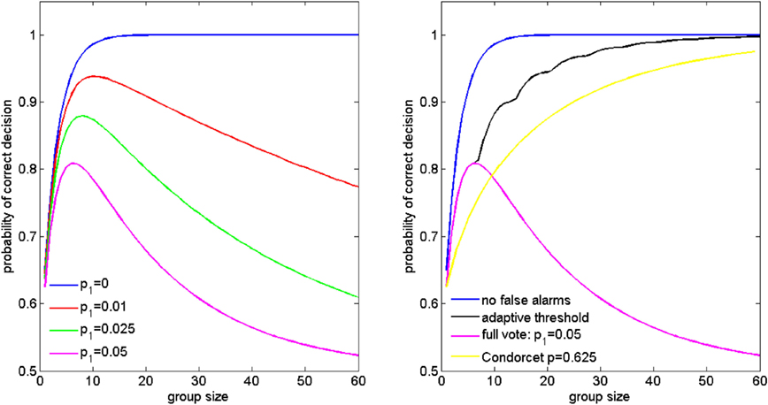
Figure A1. The effect of false alarms. Left panel: The effect of varying false alarm probability p₁ on performance of the full vote method (p₂ was fixed at 0.3 for all curves on the panel). Right panel: performance can be restored if we allow the decision threshold T to vary as group size N changes. Black curve demonstrates how even with false alarm probability p₁ = 0.05, we can rescue performance if we choose the optimal T for each N. The yellow curve gives the performance of the group if all members were statistically independent (Condorcet) so as to show that small false alarm probabilities do not disrupt the ability to make gains as compared to the independent agent scenario.

If the threshold value was T, then the probability of a correct decision was given as $p\left(\mathit{correct}\right)=\frac{1}{2}\mathit{sumP}\left(T,N,p1\right)+\frac{1}{2}\left(1-\mathit{sumP}\left(T,N,p2\right)\right)$, where $\mathit{sumP}\left(T,N,p\right)={\sum }_{m=0}^T\frac{N!}{m!\left(N-m\right)!}{p}^m{\left(1-p\right)}^{N-m}$. For the adaptive threshold method, the value of T was calculated as $T=⌊\left(N\frac{\mathit{ln}\frac{1-p_1}{1-p_2}}{\mathit{ln}\frac{\left(1-p_1\right)p2}{\left(1-p_2\right)p1}}\right)⌋$, where N is again the group size and ⌊ x ⌋ indicates the floor value of x. This expression for T was derived from the condition that sumP(T, N, p₁) > sumP (T, N, p₂).

3. Modeling the Influence of Distracting Alternatives

In this section, we map both our distracter method and Condorcet voting onto a diffusion process. We then show that the distracter scenario is a generalization of Condorcet theorem which also guarantees higher performance for all values of N > 1 and K > 2.

Let us first restate our assumptions. Our decision-makers are randomly sampled from an infinite crowd, where a fraction k of individuals are experts who always vote correctly no matter how many alternatives they face. The remaining fraction 1 − k of uninformed individuals each choose one option among the K alternatives at random. The uninformed individuals choose independently from each other. Out of the K alternatives, two are credible candidates for the correct option while K − 2 are distracting alternatives. Only the central decision-maker knows which alternatives are the irrelevant distracters, the voters remain ignorant of their existence.

During each round, we sample N individuals and have them vote. After the vote, we discard all the opinions that landed on the K − 2 distracting alternatives. Our final decision will be chosen according to which of the two alternatives that we considered realistic candidates for an answer received more votes. If both alternatives receive equal support, then we toss a fair coin to determine our final opinion.

First, it is clear that for the case of K = 2, the probability that a randomly chosen individual gives the correct answer is $p=k+\frac{1}{2}\left(1-k\right)$. The voting under this scenario is equivalent to regular Condorcet voting since we have no irrelevant alternatives. This scenario will act as our baseline. We now show that as we increase K to values larger than 2, we outperform this baseline (for any value of N > 1).

We can view our voting procedure as a diffusion process. We are interested in the value δx, which measures the difference between the number of votes casted for the correct alternative relative to the number of votes casted for the incorrect alternative. After N votes have been cast, if δx > 0 then we have made the right choice. If δx = 0, we choose correctly with probability $\frac{1}{2}$. Otherwise we make a mistake.

During a single round of voting, δx acts as a random variable. With probability k, we sample an expert and δx increases by 1. In the 1 − k cases, where we miss the expert, we have two mutually exclusive alternatives. With probability $\frac{2}{K}\left(1-k\right)$, we add to δx a random variable s which has value 1 with probability $\frac{1}{2}$ and value −1 also with probability $\frac{1}{2}$. This corresponds to a case where one of the uninformed individuals lands a vote among one of the two credible alternatives. With probability $\frac{K-2}{K}\left(1-k\right)$, the value of δx remains the same as the vote of an uninformed individual lands on one of the distracters.

We can see that δx evolves as the sum of three mutually exclusive variables: the signal variable, the noise variable and the neutral variable. The probability of sampling the signal variable remains the same for all values of K. But the probability of sampling the noise variable decreases as a function of K. This gives the intuition why Condorcet scenario of K = 2 gives the worst performance. It happens because the signal-to-noise ratio is at its lowest value. We next give a more formal proof of our statements.

As can be seen from previous discussions, the probability of sampling an expert’s opinions remains unchanged as K varies. In what follows next, the values of k and N will be fixed. Therefore, for all values of K, we can write

$p_w\left(K\right)={\displaystyle \sum _{q_e=0}^N}p\left(w|q_e,K\right)p\left(q_e\right),$ (A5)

where p_w(K) is the overall probability of the group making an incorrect decision for a fixed value of K, p(q_e) is the probability that a sample of N opinions will contain q_e expert opinions, and p(w|q_e, K) gives the probability of making an incorrect decision given that the sample of N opinions contained q_e experts. Note that the quantity p(w|q_e, K) depends on K.

The next step in our proof is to show that p(w|q_e, K = 2) ≥ p(w|q_e, K > 2) for all values of q_e. Essentially, we will show that no matter how many experts a particular sample contained, adding more irrelevant alternatives always reduces or leaves the probability of error the same. The conclusion then follows immediately from considering equation (A2).

For K = 2 and q_e, we know that the number of noise opinions is fixed at q_n = N − q_e. Therefore, p(w|q_e, K = 2) = p(w|q_e, q_n = N − q_e). For values of K larger than 2, the number of noise variables for any given sample containing q_e experts is not fixed, but varies between 0 and N − q_e depending on how many of the variables were neutral variables because the opinions landed among the irrelevant distracters. Therefore, for K > 2, we may write

$p\left(w|q_e,K\right)={\displaystyle \sum _{q_n=0}^{N-q_e}}p\left(q_n|q_e,K\right)p\left(w|q_n,q_e\right).$ (A6)

From equation (A3), we can see that the inequality p(w|q_e, K = 2) ≥ p(w|q_e, K > 2) holds as long as p(w|q_n, q_e) is a non-decreasing function of q_n since ${\displaystyle \sum _{q_n=0}^{N-q_e}}p\left(q_n|q_e,K\right)=1$.

The last step of our proof is to show that p(w|q_n, q_e) is indeed a non-decreasing function of q_n. Let us compare the value of p(w|q_n, q_e) with p(w|q_n + 1, q_e). We can write p(w|q_n, q_e) as

$p\left(w|q_n,q_e\right)=\frac{1}{2}p\left(s_n=-q_e|q_n\right)+{\displaystyle \sum _{s_n=-q_n}^{-q_e-1}}p\left(s_n|q_n\right),$ (A7)

where s_n is a random variable that is calculated as the sum of q_n randomly and independently sampled noise variables which each take the values 1, −1 with probability 0.5. This equation is a simple application of the idea that in order to overturn the correct signal induced by the q_e experts, the q_n noise variables must have a sum equal to or lower than the value −q_e. The term p(s_n = − q_e|q_n) contributes half its value because ties are broken by a coin toss.

We can relate p(w|q_n, q_e) to p(w|q_n + 1, q_e) by noting that in any random sample, when moving from q_n to q_n + 1, we are simply adding a number −1 or a number +1 to the value of s_n already present in the sum. If the value of s_n was already lower than −q_e − 2, then the addition of even a +1 is not enough to overwhelm the destructive influence of the noise. Also, if s_n was already higher than −q_e + 2 then even sampling a −1 is not enough to overturn the signal. Therefore, the only terms that may have any effect concern the boundary cases of s_n = − q_e + 1, s_n = − q_e, and s_n = − q_e − 1. Putting all this together,

$\begin{array}{ll}\hfill p\left(w|q_n+1,q_e\right)& =\frac{1}{4}p\left(s_n=-q_e+1|q_n\right)+\frac{1}{2}p\left(s_n=-q_e|q_n\right)\\ & +\frac{3}{4}p\left(s_n=-q_e-1|q_n\right)\\ & +{\displaystyle \sum _{s_n=-q_n}^{-q_e-2}}p\left(s_n|q_n\right)=p\left(w|q_n,q_e\right)+\frac{1}{4}p\left(s_n=-q_e+1|q_n\right)\\ & -\frac{1}{4}p\left(s_n=-q_e-1|q_n\right).\end{array}$ (A8)

We are left to examine the term $\frac{1}{4}p\left(s_n=-q_e+1|q_n\right)-\frac{1}{4}p\left(s_n=-q_e-1|q_n\right)$, which turn out to be non-negative for all values of q_e, q_n. If q_e = 0, then the term is obviously zero because the distribution of s_n is symmetric and p(w|q_n, q_e) = p(w|q_n + 1, q_e). A similar conclusion holds if q_e > q_n because then both probabilities of the difference term are zero. The more interesting case concerns 0 < q_e < q_n + 1. In that case $\frac{1}{4}p\left(s_n=-q_e+1|q_n\right)>\frac{1}{4}p\left(s_n=-q_e-1|q_n\right)$, because the distribution of s_n peaks at zero and decreases monotonically as s_n decreases away from 0. The combination of the three cases gives us the proof that p(w|q_n, q_e) is non-decreasing in q_n which concludes our proof.

For the limit of K tends to infinity, we can give a surprising and compact expression for how performance varies with group size. For large K, nearly all uninformed opinions land on the distracter alternatives. Therefore, the only way a mistake will occur is if no experts happen to be selected into the group and the coin flip favors the wrong alternative. The probability of such an event is $\frac{1}{2}{\left(1-k\right)}^N$ and, therefore, the probability of getting the correct answer is $1-\frac{1}{2}{\left(1-k\right)}^N$ which is the same equation as we had for the many-eyes model but with k replaced by t.

4. Training Neural Networks

The neural networks were trained in Tensorflow (Abadi et al., 2016). For the first task, we used an input layer of size 30 and two hidden layers of size 75 with rectified linear activation. The cost function optimized was the mean square error. We created a simulated dataset as described in main text with 5,000 training examples. The network was trained with ADAM using learning rate of 0.01.

For the case of doctor’s estimations of presence of skin cancer, we used a dataset comprised of evaluations of 40 doctors on 108different cases of potential melanomas from Kurvers et al. (2016). We split these cases into 54 training, 27 validation, and 27 test cases. For each groups size, we trained 50 different networks using 50 different random partitions of the data into 54, 27, and 27 cases.

Accuracy of each doctor was determined computing her Youden’s index (J = sensitivity + specificity − 1) over the training cases. We then produced all 780 combinations of 2 doctors, and 1,000 random combinations of 3, 5, and 7 doctors, and computed the accuracy of each group using the different heuristics proposed over the test cases. The performance of the heuristics for each group size was then determined by averaging its value across all groups.

To train each network, we generated 54 training instances combining judgments, accuracies, and confidence ratings of each random group on each particular case. For example, for groups of 2 doctors each input was then composed of accuracy of first doctor, confidence of first doctor, accuracy of second doctor, and confidence of second doctor. Accuracies were multiplied by −1 if the doctor had judged the case as negative. We used the training cases to train the network and the validation cases to select the state of the network that produced the best performance. Then this particular state was applied to make predictions over the test cases and to compare its performance with the heuristics applied to the pairs.

The network architecture was different for each group size. For groups of 2 and 3 doctors, two hidden layers were used; and for groups of 5 and 7, only one hidden layer was used. The size of each layer was 250 for groups of 2, 5, and 7 doctors, and 100 for groups of 3 doctors. All hidden layers had rectified linear activation. The network was trained with ADAM using learning rate of 0.0001 for groups of 2 doctors and 0.00001 for groups of 3, 5, and 7.

The cost function was selected to match the accuracy measured by the Youden index. This index is of the form J = TP/(TP + FN) + TN/(TN + FP) − 1, with TP standing for true positives, FN for false negatives, TN for true negatives, and FP for false positives. As the output of the network was the probabilities p and 1 − p that the case fed was a positive or a negative, the expected value of the Youden’s index would be of the form $E\left[J\right]={\displaystyle \sum _{i=1}^{n_p}}\frac{p_i}{n_p}+{\displaystyle \sum _{i=n_p+1}^{n_p+n_n}}\frac{1-p_i}{n_n}-1$, where n_p (n_n) is the number of positives (negatives) and the first (second) sum is over the positive (negative) cases. The cost function optimized was then of the form 0.5(1 − E[J]), which is 0 at the maximum expected Youden’s index (E[J] = 1) and 1 at the minimum Youden’s index (E[J] = − 1).