Simulation-Based Internal Models for Safer Robots
 Christian Blum
 Alan F. T. Winfield
 Verena V. Hafner
- 1Adaptive Systems Group, Department of Computer Science, Humboldt-Universität zu Berlin, Berlin, Germany
- 2Bristol Robotics Laboratory, UWE Bristol, Bristol, United Kingdom
In this paper, we explore the potential of mobile robots with simulation-based internal models for safety in highly dynamic environments. We propose a robot with a simulation of itself, other dynamic actors and its environment, inside itself. Operating in real time, this simulation-based internal model is able to look ahead and predict the consequences of both the robot’s own actions and those of the other dynamic actors in its vicinity. Hence, the robot continuously modifies its own actions in order to actively maintain its own safety while also achieving its goal. Inspired by the problem of how mobile robots could move quickly and safely through crowds of moving humans, we present experimental results which compare the performance of our internal simulation-based controller with a purely reactive approach as a proof-of-concept study for the practical use of simulation-based internal models.
1. Introduction
A new generation of intelligent mobile robots is required to operate in dynamic human environments. Two examples are museum tour guide robots and hospital portering robots. For robots such as these, safety is an overriding concern. Designing control systems that assure the safety of mobile robots in human environments is very challenging, not least because humans are unpredictable. Conventional safety features for mobile robots in human environments include: moving at very low speed, flashing lights or alarms to alert humans of the robot’s presence, and having proximity sensors to detect obstacles—including humans—and to bring the robot to a complete halt. If, despite these measures, a human fails to notice the robot, then they are likely to collide. Safety therefore relies, in large measure, on the intelligence of the human rather than the robot. But if mobile robots need to move fast through crowds of moving humans, in an emergency situation, for example, then we need a much smarter approach to collision avoidance.
In this paper, we explore the potential of mobile robots with simulation-based internal models for safety in dynamic environments. We propose a robot with a simulation of itself, other dynamic actors and its environment, inside itself.
Operating in real time, this simulation-based internal model is able to look ahead in time and predict the consequences of both the robot’s own actions and those of the other dynamic actors in its vicinity. Hence, the robot continuously modifies its own actions in order to actively avoid collisions while also achieving its own goals. We present experimental results which compare the performance of our internal simulation-based controller with a purely reactive obstacle avoidance approach.
The idea of internal models can be retraced at least as far back as 1943 when Craik (1967) presented his idea of “small-scale models”:
If the organism carries a “small-scale model” of external reality and of its own possible actions within its head, it is able to try out various alternatives, conclude which is the best of them, react to future situations before they arise, utilize the knowledge of past events in dealing with the present and future, and in every way to react in a much fuller, safer, and more competent manner to the emergencies which face it.
An Internal Model is a mechanism for internally representing both the system itself and its current environment. An example of a robot with an Internal Model is a robot with a simulation of itself and its currently perceived environment, inside itself. A robot with such an Internal Model has, potentially, a mechanism for generating and testing what-if hypotheses; i.e.,
1. what if I carry out action x..? and, …
2. of several possible next actions xi, which should I choose?
Holland (1992), p. 25, writes: “an Internal Model allows a system to look ahead to the future consequences of current actions, without actually committing itself to those actions.” This leads to the idea of an Internal Model as a consequence engine—a mechanism for estimating the consequences of actions. Dennett (1995), in his book Darwin’s Dangerous Idea, elaborates the same idea in what he calls the “Tower of Generate-and-Test,” a conceptual model for the evolution of intelligence that has become known as Dennett’s Tower. Dennett’s tower is a set of conceptual creatures each one of which is successively more capable of reacting to (and hence surviving in) the world through having more sophisticated strategies for generating and testing hypotheses about how to act in a given situation.
The ground floor of Dennett’s tower represents Darwinian creatures; these have only natural selection as the generate and test mechanism, so mutation and selection is the only way that Darwinian creatures can adapt—individuals cannot. All biological organisms are Darwinian creatures. A small subset of these are Skinnerian creatures, which can learn, but only by generating and physically testing all different possible actions, then reinforcing the successful behavior—providing of course that the creature survives. On the second floor, Dennett’s Popperian creatures—a sub subset of Darwinians—have the additional ability to internally model the possible actions so that some (the bad ones) are discarded before they are tried out for real. A robot with an Internal Model, capable of generating and testing what-if hypotheses, is thus an example of an artificial Popperian creature within Dennett’s scheme. The ability to internally model possible actions is of course a significant innovation.
In biology and neuroscience, the concept of internal models is thought to be behind most of the exceptional sensorimotor skills that can be observed in nature, since it is essential for high-performance control as implemented in biological systems (Haruno et al., 2001; Wolpert et al., 2011). The use of internal models has been demonstrated in a large number of biological systems ranging from dragonflies (Mischiati et al., 2015) to humans (Flanagan et al., 2001). Indeed, it has been proposed that thinking—including anticipation—is “simulated interaction with the environment,” in what is known as the simulation theory of cognition; see the influential work of Hesslow (2002, 2012).
In previous work, we proposed a simulation-based internal model architecture (Winfield, 2014) centered upon what we call a Consequence Engine (CE). To demonstrate the effectiveness of the CE approach for safety, we have undertaken a series of experiments involving one smart (as in using a CE) robot and several other (i.e., Braitenberg style) robots acting as proxy-humans in our scenario. The goal of the smart robot is to move as quickly as possible from one end of a corridor to the other while safely avoiding the proxy-human robots which are moving around randomly. In this paper, these proxy-human robots will be referred to as h-robots.
However, this work is not intended as an engineering solution to this particular problem of safety in human–robot interaction (HRI). At best, the other robots in this scenario can be seen as proxies for humans who are not paying attention because they are absorbed in using their smartphones while walking on the sidewalk. Instead, this scenario is used as a case study and proof of concept for the use of a CE in HRI. In particular, it is designed to include higher order interactions in addition to the interactions between the robot running the CE and other robots, which were the focus of Winfield et al. (2014). Interactions between robots and the environment are called second-order interactions, and interactions between other robots third-order interactions. Second-order effects were addressed by choosing a narrow corridor for the experiment and third-order effects were addressed by employing a sufficient number of other robots in the confined space of the corridor to generate high robot density. Nevertheless, we believe that the concept of a CE has the potential to be an effective means to accomplish improved safety in HRI scenarios. The way in which the conditions needed to test the CE naturally led to an experiment resembling conditions for HRI safety strengthens this belief.
This scenario is illustrated in Figure 1 showing a possible initial condition for the experiment as well as one possible safe solution.
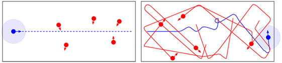
Figure 1. Illustration of the task. A smart robot (marked in blue) using the consequence engine CE has to traverse a corridor from left to right without colliding with the h-robots (marked in red). Solid lines show the past trajectories, and arrows represent the current movement direction of the robots. The light blue circle around the smart robot marks a safety (exclusion) zone. The left panel shows a set of initial conditions with the task depicted as a dashed line. The right panel shows the realized trajectories at the end of an episode of the experiment.
2. Materials and Methods
2.1. Internal Model-Based Consequence Engine
2.1.1. Architecture
The architecture discussed here is based upon the Consequence Engine (CE) (Winfield, 2014; Winfield et al., 2014; Vanderelst and Winfield, 2017). A schematic view of this architecture is shown in Figure 2. The CE allows the robot to evaluate the consequences of each of its next possible actions, which are executed inside the simulator contained in the CE using an internal model, after which the consequences of every action are evaluated in turn. This process is relatively independent of the robot’s controller in that the CE only provides estimates of the consequences of the next possible actions but the robot itself chooses and then executes the next action in the real world. The CE thus acts to moderate the robot controller’s action selection mechanism.
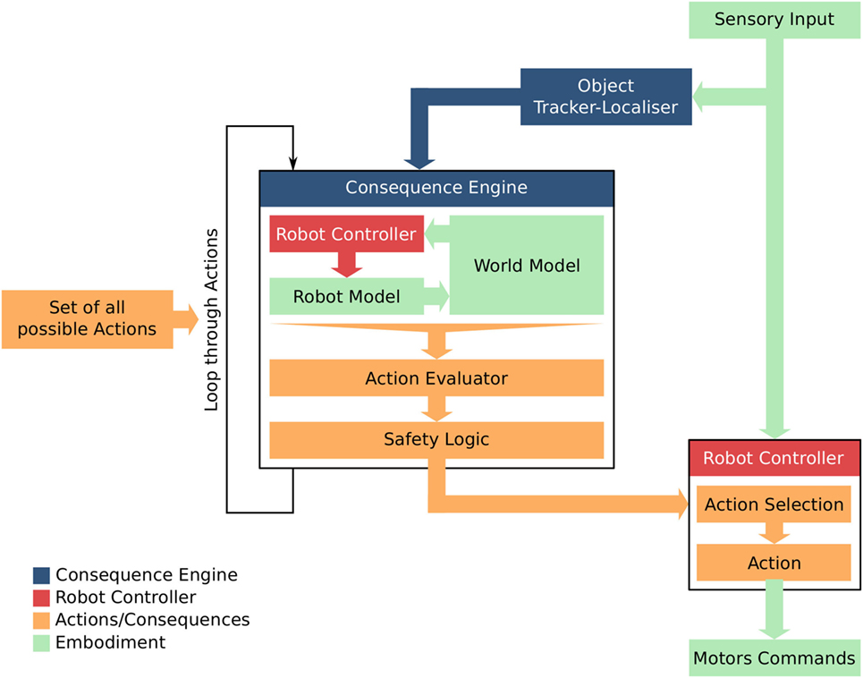
Figure 2. The Consequence Engine (CE) architecture, and its relationship with the robot’s controller. Modules dealing with different kinds of information are color coded.
The CE architecture consists of several modules. The CE is initialized with information about the current situation by the Object Tracker-Localizer (OTL) then loops through all possible next actions. In the simplest case, this set of actions is fixed by design but it could as well be dynamically generated. For each candidate action, the CE simulates the robot itself executing the action, as well as all other entities tracked by the OTL and described by the internal model, as well as the environment. It thus generates a set of simulation outputs, such as, for example, trajectories of all agents, which are then evaluated by the Action Evaluator (AE). The evaluations of the physical consequences performed by the AE are then passed to a separate Safety Logic (SL) module implementing the definition of safety as defined by the specific task. This evaluation results in a safety value (cf. Section 2.2 for details) for each action. Once the CE has generated a complete set of consequences and their evaluation in the form of safety values, all next possible actions together with their corresponding safety values are passed to the Action Selection (AS) mechanism of the robot. This AS module then selects one of the actions according to this evaluation for execution by the robot controller.
2.1.2. Modules
The AE, SL, and AS are discussed in detail in Section 2.2 in the context of the set of possible actions and their corresponding safety values.
2.1.2.1. Object Tracker-Localizer
The OTL has been implemented using a commercial motion capture system and fitting the robots with reflective markers. The motion capture system supplies the robot with position and pose data for all robots. This system is discussed in more detail in Section 2.4.5. In principle, this module could also be implemented locally on the robot using a camera and computer vision, or by all agents broadcasting their own position and orientation.
2.1.2.2. Simulation-Based Internal Model
The simulation-based internal model comprises three modules: the Robot Model, Robot Controller, and World Model. The Robot Model is a model of the robot running the CE as well as all other robots, The Robot Controller is a duplicate of the robot’s real controller, and the World Model is a virtual duplicate of the environment. After it has been initialized with the current situation by the OTL, i.e., the environment and pose of both the smart robot and all other robots in the environment, the simulation-based model can generate simulated trajectories and any consequences, i.e., collisions. The internal model and its implementation in this research is described in detail in Section 2.3.
2.1.2.3. Action Evaluator
The AE checks the trajectories generated by the internal simulation for each action against the safety action defined as a part of the task of the robot. It labels the actions as safe or dangerous and passes this information on to the SL. For more detail on the safety definition used in the experiment and the AE itself, refer to Section 2.2.1.
2.1.2.4. Safety Logic
The SL combines the information about the safety for each action from the AE with the task description of the robot in the form of the base value and assigns a safety value for each action by modifying the corresponding base value. This module weights the safety of an action against how well the action performs the task of the robot. A more in-depth discussion on how the SL combines these two aspects can be found in Section 2.2.3.
2.1.2.5. Action Selection
The AS selects an action from the set of possible next actions according to their safety value. Ordinarily, this means that it chooses the action with the best safety value. The practical meaning of this choice in the context of the experiment is discussed in Section 2.2.4.
2.2. From Actions to Safety Values
2.2.1. Safety Definition and Action Evaluator
To be able to decide which actions to use, a safety concept is needed. A very simple measure was chosen in order to make the decision process as transparent as possible to facilitate experimentation and debugging.
An action for a robot is considered safe if no other robot or obstacle such as a human1 is closer to it than some safety distance for any given time. The safety distance was chosen to be 0.22 m (refer to the end of Section 3 for a short discussion on the specific value of this parameter). This safety distance is intentionally chosen to be considerably larger than the range of the IR sensors of the robots.
In the context of the CE architecture, this means that the AE has to check for every possible next action that no other robot gets closer than this safety distance for any given time using the predicted trajectory obtained by the simulation. The AE therefore literally evaluates the consequences of each possible action for this safety criterion.
Note that these predicted trajectories are not simple ballistic continuations of the current pose and speed of the h-robots for a given action but also take into account what can be called second order effects, i.e., interactions of the robots with the environment, and third-order effects, i.e., interactions between robots. In this regard, the approach introduced here goes beyond most biologically inspired internal models considered in literature, which are mostly body and physics models and do not take interaction into account.
2.2.2. Task Description and Action Space
The task of the smart robot is described using Potential Functions (PFs) (cf. Spears and Spears (2012) for an introduction to the concept). The PF encodes the goal of where the smart robot is to move toward and also the preferred way of getting there, effectively following the gradient of the PF. In this particular experiment, the task of the robot is to move from one end of a corridor to the other end of the corridor. This task is described by the PF
This PF describes a trough with an incline from the start to the goal of the robot. The parameters were chosen in a way to encourage movement toward the goal and at the same time slightly discourage movement away from the shortest path from the starting point to the goal, which is the trajectory used by the baseline experiment in our proof-of-concept experiment (cf. Section 2.4). To limit the set of possible next actions to a finite number, this PF is sampled on a 6 × 3 grid with dimensions of 2 m × 0.8 m to create the set of next possible actions for the smart robot.2 This limits the set of next possible actions to a finite number of actions. Each of these actions is formed of the sub-actions MoveTo(x,y) and Avoidance (cf. Section 2.4.4). Even though this set of actions is discrete, the overall behavior of the robot is continuous and since the CE operates at about 2 Hz on the computer used for the simulations, the robot can change the current action several times between moving from one grid point to another, effectively interpolating its actions between the grid points. This also means that the robot can in principle move to and stop at any grid point. However, this behavior is highly unlikely as this means that all other actions with a MoveTo(x,y) grid location closer to the goal have to be classified by the CE as resulting in an unsafe situation for the time it takes the robot to move to and stop at the grid location, which is a possible but unlikely scenario as the other robots constantly move.
The values of the samples from the PF on this grid for the respective actions are the so-called base values of these actions. The choice of PFs to generate these base values is arbitrary and could as well be substituted by any number of other ways to assign a value to an action depending on the task the robot is to perform.
As these base values and the set of possible next actions define the task of the robot, they are chosen by the designer of the robot. However, in principle, they could also be generated dynamically by an algorithm.
2.2.3. Safety Values and Safety Logic
Safety values are generated by the SL based on the results of the AE and describe the safety of an action. In this work, these safety values are represented by scalar values but could in principle also be represented by something more expressive such as a vector of different safety values to describe different kinds of safety (safety of the robot, safety of other robots, safety of humans).
The scalar safety values used in this work consist of two parts: the base value and the safety modifier. As described in Section2.2.2, the base value encode the default task of the robot to be followed if no danger is imminent while the SL adjusts the base value with a safety modifier if the AE detects imminent danger according to the safety definition (cf. Section 2.2.1).
This assessment is performed by the SL according to the specific safety definition, which in practice severely discourages any actions failing those safety conditions by modifying the safety value, effectively pruning these actions from the set of possible next actions. A safety modifier of −100 maxactions (s(x, y)) added to the base value of an action, for which the AE has detected danger, is a typical choice as it ensures that the penalty of a dangerous action is much larger than the base values.
If more complex decisions have to be made by the robot, the rules employed by the SL can also be used to weigh several factors against each other. In the context of this work, safety values consist of a base value defined by a PF and a safety modifier as described in Section 2.2.2. In this case, the step of the SL modifying the base values with safety modifiers can in principle also be performed before discretizing space by modifying the PF and therefore the base values directly.
2.2.4. Action Selection
The AS of the robot chooses the action with the best, i.e., highest, safety value. In this experiment, that means the action, which follows the gradient in the modified PF while avoiding dangerous situations. Note that the AS is part of the robot controller, and the robot can thus also in principle choose to select actions with a worse safety value than the safety value of the best action as determined by the SL.
2.2.5. Putting Everything Together
The complete process is depicted schematically in Figure 3. It starts with the set of possible actions and a PF defining the task of the robot moving to the right end of the corridor. The CE then loops through this set and generates trajectories for both the smart robot and the h-robot (in this example, there is only one h-robot). The AE then checks the trajectories for danger according to the safety definition and the SL combines this information with the base values (as described by the PF in this example) to assign safety values to the action. The AS of the robot then chooses the action with the best safety values.
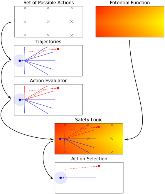
Figure 3. Example of how an intelligent robot running a CE chooses the best action from the set of possible actions and the base values using the AE and SL. The panel Potential Function depicts a color coded rendition of the example potential function. Furthermore, the panel Set of Possible Actions depicts the discretization of space employed. The simulated trajectories for all actions in the set of possible actions generated by the internal simulator are depicted in the panel Trajectories. The trajectories of the intelligent robot are depicted as solid blue lines and the ones of the other robot as red dashed lines, respectively. Because of the finite time simulated ahead, the trajectories of the intelligent robot do not reach the designated targets of the actions for the three most distant targets. Note that the trajectories of the other robot are identical for most of the actions, which is the case if the two robots do not interact, so the lines lie exactly on top of each other. The panel Action Evaluator depicts the evaluation of the trajectories by the AE by coloring the trajectories red for which a safety violation is detected. The SL combines the results of the AE with the PF, which is represented graphically by overlaying the corresponding panels in Safety Logic. The last panel Action Selection depicts the action selected for execution by the AS of the robots by only showing the corresponding trajectories of the two robots.
2.3. Internal Simulator
The internal model is implemented using a slightly modified off-the-shelf simulator (cf. Section 2.3.1). All models of other robots and the environment are hard-coded to simplify the experiment in order to be able to focus on the architecture itself. In principle, all models, i.e., world model as well as model for other entities and so on, could also be based on a learned internal model.
In general, simulations used in robotics often use advanced physics and sensor models, to test and develop robots and the corresponding controllers before they are implemented in hardware to save development time and reduce the risk associated with bugs, faults, and failures. Examples of standard robotic simulations include Gazebo (Koenig and Howard, 2004), Webots (Michel, 2004), Player-Stage (Vaughan and Gerkey, 2007), and Morse (Echeverria et al., 2011). When using a simulator, the so-called reality gap (Jacobi et al., 1995), created by the approximation of the performance of real sensors and actuators by the simulator by the respective sensor and motor model, has to be taken into account. This topic will be further discussed in Section 2.3.3.
2.3.1. The Stage Robot Simulator
The simulator running the internal simulation is a modified Stage simulator (Vaughan and Gerkey, 2007; Vaughan, 2008). It was modified to act as simulation server in a service-oriented architecture accepting SimRequest messages (cf. Figure 11) over a network. These requests consist of a number of robots, their initial poses, the configuration for their controllers, and the simulation time. Upon execution, the server returns complete trajectories for all robots for the simulation time. This also means that in a typical situation, where the CE has to run numerous simulations to loop through the set of possible next actions, the available simulation power can be arbitrarily scaled up by employing several simulation servers and a transparent load balancer.
The simulation contains a copy of the environment, the robots used, their sensors, and their controllers. The controllers execute exactly the same code as the real robots and the sensors and motors are calibrated to the real ones empirically. In principle also, learned robot models and controllers could be used. The performance of the simulation and the resulting simulation budget is discussed in Section 2.3.4.
2.3.2. Decision Search Tree
Most internal model-based architectures in robotics perform only a projection of one time-step into the future, especially when dealing with learned body models. In this work, the goal is to simulate much further—possibly several orders or magnitude—into the future than one time-step employing the speed and precision of the off-the-shelf simulator and full knowledge of the world.
As depicted in Figure 4, these multistep simulations lead to search trees if the robot can perform more than one action since it can in principle decide during each time step to change the current action. Performing simulations of only one step and doing depth-only search are two extremes of traversing the full decision tree. Searching a full decision tree is not practical because of the curse of dimensionality, so some sort of pruning has to be devised, especially for deeper searches. Choosing a depth-only search as used here in contrast constitutes one of the most simple and straightforward ways of accomplishing that goal. Using depth-only search is a valid simplification if the robot controllers in the simulation are stateless (cf. Section 2.4.4).
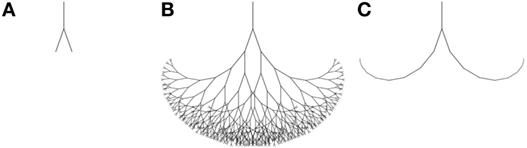
Figure 4. Schematic search trees for a one step search (A), full search (B), depth-only search (C) resulting from multistep simulations.
2.3.3. Reality Gap: Simulation Error Measurements
There is a reality gap between every simulator and the physical object it represents. To measure that gap, six robots were used in the arena described in Section 2.4.5 executing the simple action GoStraight(0.8);Avoidance. Their trajectories were recorded for 489 s. The resulting real trajectories are depicted in Figure 5.
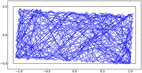
Figure 5. Trajectory of a robot performing the test action for 489 s used for the simulation error calibration. The measured trajectory of the robot is depicted as a blue line, and the location of the arena walls in the frame of reference of the simulation is depicted as a black line. The mismatch between the area formed by the trajectory measurements and the arena show the calibration error of 3° of the motion capturing system.
From the mismatch between the trajectories and the arena walls, it is obvious that the calibration of the motion capturing system placed its coordinate system rotated by about 3° and also slightly offset. This is due to the calibration process of the motion capturing system using a manually placed ground plate with markers to establish the motion capturing coordinate system.
Simultaneously, the movement of the robots was projected into the future via simulation for different simulation times. After finishing the experiment, the error between the simulated trajectories and the actual real trajectories was calculated for all time steps and simulation times. The results are depicted in Figure 6.
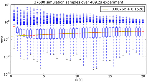
Figure 6. The simulation error is depicted as a function of simulation time on a logarithmic scale. A linear model for the median as a function of simulation time is also shown as a yellow line.
The figure shows normalized errors, which means that the cumulative error is divided by the length of the real trajectory. Thus, there are numerical errors for small simulation times as the measured error is divided by a small number, so the increased error for short simulation times is a purely numerical artifact. For longer simulation times, there is a linear increase in the median error, which is most probably due to the misalignment between the motion capturing coordinate system, which is the same as used for the simulation, and the real coordinate system. This error is far larger than the one caused by inaccuracies of the simulation, which are expected to be scaling roughly quadratic in time.
In general, simulation errors are mitigated to some extent by the fact that the CE, which is running at 2 Hz, is periodically updating the simulations it performs by new simulations in a memoryless fashion discarding old simulation results. As seen in Figure 6, the simulation error is the smaller the shorter into the future an event is occurring. This means, for example, that the closer two robots get, the better the predictions of a possible interaction becomes.
The virtual sensors of the simulated robot, in particular the IR sensors, have to be calibrated to the real sensors. This calibration was performed with a focus on reproducing the behavior of the real robot, i.e., turn rates and radii when performing avoidance behavior close to walls and other robots. However, the particular calibration employed here led to the effect of simulated robots getting stuck on walls or in rare cases on other robots.3 This effect occurs only for long simulation times and only rarely. In real experiments, measurement errors and motor, i.e., movement, noise of the real robots mitigates this effect completely. For pure simulations in contrast, i.e., simulated robots using a CE to internally simulate other simulated robots, this effect can be observed in 10–20% of experiments. This effect is only relevant for the simulation study performed in Section 3 as all other experiments were conducted with real robots. For this study, the simulation runs in which this effect occurred were discarded while performing the statistical analysis so they have no effect on the statistical validity of this study.
2.3.4. Simulation Budget
The CE runs at approximately 2 Hz so there is a budget of 0.5 s to loop through all possible actions, simulate their outcome, asses the consequences, assign a safety value to each action, and then choose the best possible action. In relation to the computational power necessary for the simulation, the other tasks are negligible, so for simplicity they are not considered for the analysis.
As mentioned in Section 2.3.1, simulation time runs at about 600 times real time on the used hardware configuration,4 so 300 s can be simulated effectively during one update cycle. This simulation time is the simulation budget which has to be allocated to the different possible next actions.
Considering the maximum speed of an e-puck robot of about 0.1 ms−1, simulation times should be roughly in the range of about 10 s in order to give the robot running the CE a chance to avoid other robots, which corresponds to 1 m traveled distance at maximum speed. This means that the simulation budget is about 30 different future actions.
As discussed in Section 2.4.2, the arena used in the experiment (2.2 m × 1.8 m) is discretized into a grid of 6 × 5 points to generate the set of possible actions. Assuming a simulation time of 10 s, this already completely saturates the simulation budget.
This is the reason why some modifications to the implementation have been performed, adding heuristics to use the simulation budget more efficiently. These heuristics are discussed next.
2.3.5. Attention Mechanism
The naive implementation loops the consequence engine through all possible actions. This is in principle the best possible option but not always feasible because of limited computational resources, i.e., the limited simulation budget. Furthermore, the simulation error (cf. Section 2.3.3) increases with time, so it might not make sense to simulate areas far away, which also implies long simulation times, since no significant information can be gained because of the large simulation error before an interaction actually occurs.
To address these issues, a simple heuristic in the form of an area of attention around the robot was implemented. Actions with goals outside of this attention area are not considered by the consequence engine. Furthermore, other robots outside of the attention area are not simulated to make more efficient use of the simulation budget. Coincidentally, this also leads to a more realistic virtual sensing of other robots since it is similar to a limited sensing radius.
The shape and size of the attention area chosen are depicted in Figure 7. As a comparison, the size of the safety area used in the safety definition (cf. Section 2.2.1) of the experiment is also shown and the physical size of the robot depicted is to scale.
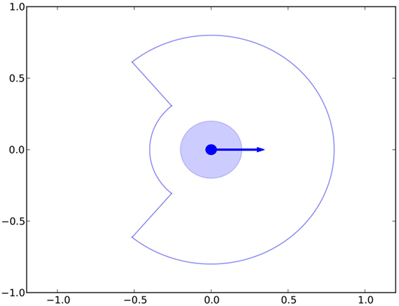
Figure 7. The area of attention used by the CE is indicated by a solid line. Also shown is the area defined by the safety radius as the lightly blue shaded area.
The size of the attention radius was chosen purely based on empirical knowledge gained in simulation. The shape of the attention area was chosen to be similar to the ones often encountered in prey animals with a reduced radius at the opposite side of the direction of movement. This choice was purely empirical but seems justified since the robot is always trying to move toward its goal so it is moving away from other robots behind itself. The shape and size of the attention radius could be optimized but performance was well within desired design criteria so this avenue of optimization was not further pursued.
2.3.6. Adaptive Simulation Time
The amount of time simulated into the future is a further parameter of the architecture. On the one hand, there is a minimum viable simulation time dictated mainly by physics in that the robot needs enough time to be able to react and avoid another robot. On the other hand, very long simulation times lead to high prediction errors because of imperfectly measured initial conditions and an imperfect simulator, making them not feasible even in a situation where computational resources are no limitation.
Furthermore, simulating too far into the future also poses a problem as it increases the probability of a dangerous situation. A very similar result has been obtained in a simulation study with virtual e-puck robots for a different task (Johansson and Balkenius, 2008). Simulating infinitely far into the future would lead almost certainly to a dangerous situation, resulting in an effectively paralyzed robot as all possible future actions ultimately lead to danger. This issue could be resolved by using a discount factor for the safety modifiers in the SL discounting dangerous situations which are further into the future (cf. Section 2.2.3). However, as the simulation times are limited to the order of 10 s by the computational resources available at the time of this experiment, dangerous situations farther into the future than this simulation time are discounted naturally by not being considered at all.
A simple heuristic was designed to dynamically adapt the simulation time using the simulation results themselves. For that, minimum and maximum simulation times (in this experiment 7.5 and 15 s) are fixed. The simulation times are adapted for each possible action individually while looping through the set of all possible actions. If a particular action does not lead to a dangerous situation, the simulation time is increased by 50% for the next update, and if it leads to a dangerous situation, it is decreased by 20% and the simulation is re-run immediately. Both increase and decrease of simulation times are limited by the minimum and maximum simulation times. The asymmetry between increase and decrease is a balance between the limited simulation budget and the necessity to react to a dangerous situation as fast as possible and the desire to maximize performance of the overall algorithm by not choosing too short simulation times.
2.4. Evaluation Experiment
In this experiment, a smart robot using the consequence engine (CE) has to traverse a corridor from left to right without colliding with the five other moving h-robots of which the controller is known to the smart robot. In this work, the same controller model applies to all robots since they are identical. As introduced in Section 1, these five h-robots can be regarded as proxy-humans, for example, in a hospital corridor. An illustration of the task can be seen in Figure 1, and the corresponding experimental setup is depicted in Figure 8.
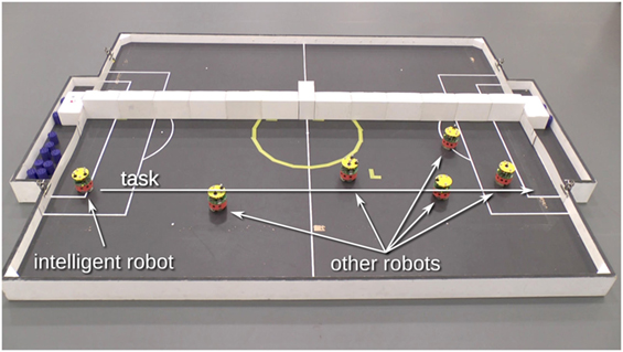
Figure 8. Experimental setup of the corridor with one smart and five h-robots. The smart robot is required to move from the left end of the corridor to the right, as indicated by the task arrow, avoiding the other h-robots which are also moving in the corridor.
Human behavior is vastly more complex than the one of the simple robots used in this experiment. However, research has shown that in some situations, such as, for example, in escape panic situations (Helbing et al., 2000) or even in the simple situation of pedestrians on a sidewalk (Helbing and Molnar, 1995), humans can be modeled very simply or with simple swarm rules. More complex models for human crowds exist (Musse and Thalmann, 1997). This makes it reasonable to use the simplified behavior of the proxy-human h-robots as a starting point of the investigation of internal models for safety purposes. In future work, more sophisticated models of humans, possibly learned by the smart robot, should be investigated. These models should include controllers, physical models, and intentions of the humans.
2.4.1. Experimental Overview
The experimental setup consists of six e-puck mobile robots (cf. Figure 10) moving in a rectangular arena of 2.2 m × 1 m. This scenario is depicted in Figure 8.
Units in this section are [m] and [rad], respectively, if not stated otherwise. The origin of the coordinate system is placed in the center of the arena and the axes are parallel to the walls of the arena with the x-axis parallel to its long side and pointing toward the goal of the smart robot.
2.4.2. Infrastructure and Physical Setup
Figure 9 shows the physical setup consisting of an arena of size 2.2 m × 1.8 m, a motion capture system, and an overhead camera.
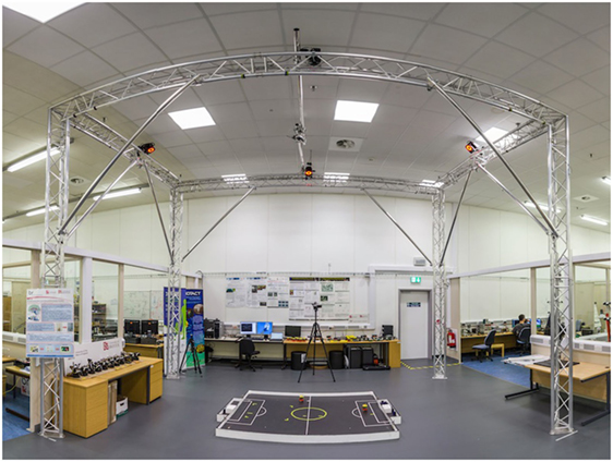
Figure 9. Experimental infrastructure showing the arena on the bottom, the camera used to document the experiments, and the Vicon motion capturing system overhead.
The off-the-shelf motion capturing system5 running at 50 Hz implements the OTL and broadcasts the positions of all robots via simple UDP messages to all participants of the wireless network at a reduced rate of 15 Hz (cf. also Figure 11). This reduced rate was chosen to be slightly faster than the internal operating loop of the robots, which runs at 10 Hz in order for the newest position measurement not to be older than the last control loop iteration mimicking the infrared sensors of the robots. The communication between the robots and the simulation server and between sub-components is based on the Google Protocol Buffers library6 and executed via TCP. All robots, the simulation server, the tracking system, and the logging system are connected via an IEEE 802.11 g wireless network in infrastructure mode. Additionally, a video camera is recording the experiments for later analysis and demonstration.
2.4.3. Robots
E-puck mobile robots (Mondada et al., 2009), equipped with a Linux extension board (Liu and Winfield, 2011), were used as a mobile base. Additionally, optical markers are arranged in individual patterns on top of the robots to facilitate tracking with the motion capture system. Two of the robots are shown in Figure 10.
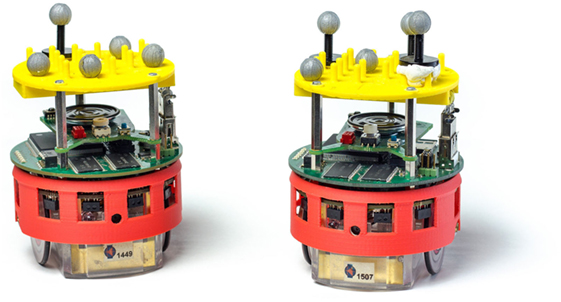
Figure 10. Two e-puck robots with markers and IR sensors. The e-puck with Linux board fitted in between the e-puck motherboard (lower) and the e-puck speaker board (upper). Note the yellow “hat,” which provides a matrix of pins for the reflective marker spheres, which allow the tracking system to identify and track each robot.
The robots are equipped with infrared sensors, which are used for basic obstacle avoidance, a camera, which is not used, and virtual sensors to sense their own pose and that of all other robots. These virtual sensors are simulated making use of the broadcast position messages of the motion capturing system.
2.4.4. Robot Controllers
All robots run a stateless controller with a fixed set of sub-actions. Those sub-actions are as follows:
• GoStraight(speed): move straight with a maximum speed of 1 ms−1
• Avoidance: Braitenberg style avoidance using IR sensors
• MoveTo(x,y): move to coordinate (x,y) using the virtual global position sensors.
Additionally, there are sub-actions not used during experiments but for the automated experimentation such as for moving robots into initial poses or related to hardware calibration and debugging and so on:
• Stop: do nothing
• TurnLeft(speed): turn left with speed
• TurnRight(speed): turn right with speed
• CalibrateIR: calibrate IR sensors
• ResetDSPIC: reset the basic robot microcontroller board
• PrintProximityValues: print the values measured by the IR sensors to stdout.
Actions are composed of a number of concatenated sub-actions and are executed at 10 Hz by the robots, independently of each other and independently of the CE. These actions form the vocabulary used for the set of all possible actions. The simulated robots in the CE run exactly the same code as the real ones, also at 10 Hz in simulated time, i.e., faster than real time.
2.4.5. Experimentation-Centered Implementation
Figure 11 shows the flow of information between the different modules of the implementation of the architecture described in Section 2.1. There are some organizational differences to the abstract architecture (compare Figure 2).
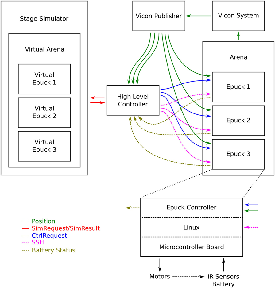
Figure 11. Flowchart of the complete experimental system including all the logging, book-keeping, and status messages used for experimental control and logging. This diagram not only contains all the elements needed for the CE but also all elements needed for automated experimentation so there are more control- and logging messages than would be needed for the operation of the CE.
The main difference to the abstract architecture is the high-level controller. This module contains the CE, the SL, and the AS of the smart robot as well as all the logging, book-keeping, and experimentation tools. The simulation server is also run on the same computer. It is very centralized for the sake of experimentation efficiency, i.e., mainly the logging of trajectories, safety values, and decisions. Since it also manages the automated experimentation, it can control all the robots used in the experiment. This feature is only used between experiments to set up new initial conditions and so on by changing the control actions for the low level controller (cf. Section 2.4.4), effectively remote controlling the robots on a high level in the sense that the robots still perform the actions completely independently of the high-level controller. In Figure 11, this mechanism is represented by the flow of CtrlRequest messages from the high-level controller to the robot controllers. While experiments are run, the different robots act completely independently of the high-level controller. Only the smart robot is influenced by the outcome of the AE.
This implementation choice however does not constitute a functional difference to the abstract architecture and could as well be implemented on the robots themselves (with some complications for the logging system).
Thus, the high-level controller, i.e., the CE, and the simulation server described in Section 2.3 are run on the same computer.7 The high-level controller of the architecture, i.e., the consequence engine, is implemented in Python. The low level robot controllers and the simulation are implemented in C/C++.
2.4.6. Initial Conditions and Goal
The smart robot is placed in an arena of size 2.2 m × 1 m at the initial position (−1, 0) oriented toward the far end of the arena and is to proceed to the other end of the arena at (1, 0) with a maximum speed of 0.1 ms−1. Furthermore, a safety radius of 0.22 m around the smart robot was chosen.
Five other h-robots are placed randomly in the area [−0.5, 1.0] × [−0.3, 0.3] with random orientations and a minimum distance to each other of 0.3 m. They execute the simple action GoStraight(v);Avoidance with random but fixed speeds randomly drawn from the interval v ∈ [0.6, 0.8]. This way the h-robots start with distances between each other and the walls larger than the range of their infrared sensors (used for avoidance behavior) and far enough from the robot running the CE to give it a clear start before having to avoid the other robots, as the maximum simulation time was chosen to correspond to about 1.0 m of movement of a robot at maximum speed (cf. Section 2.3.4).
As a baseline experiment, the smart robot moves straight toward the goal using only its IR sensors for avoidance. Consequently, this strategy leads to a high probability of another h-robot entering the safety radius even though actual collisions are avoided using the avoidance behavior. This naive baseline strategy is then compared to the one using the CE. To increase comparability between the two approaches, all experiments are initialized with the same initial conditions for both approaches. The initial conditions between pairs of approaches are randomized as described above.
Furthermore, the roles of the six physical robots in the experiments are chosen randomly to be either a smart robot or an h-robot to mitigate inter-robot heterogeneity between each pair of experiments (baseline and CE approach).
In addition to the real robot experiments, the experiments were also repeated purely in simulation. Thus in total, four types of experiments (baseline real, CE real, baseline simulation, CE simulation) were conducted, which were repeated 54 times (real) and 88 times (simulation), respectively.
3. Results
One example run of the experiment is depicted in Figure 12. Shown are snapshots of the experiment with the predicted trajectories for both the smart robot and the other h-robots from the point of view of the smart robot. The CE loops through all possible actions, but for clarity, only the simulated trajectories for the best action, which was then selected by the AS, are shown.
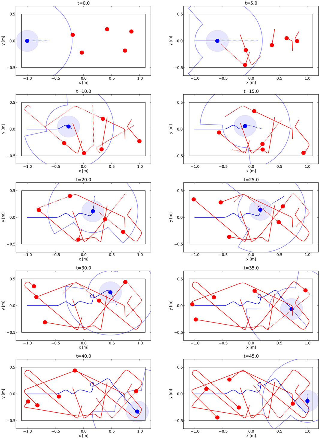
Figure 12. Trajectories for one experiment with a smart robot in simulation (for real experiments, please refer to Videos S1–S5 in Supplementary Material). The smart robot is depicted blue and the h-robots red. Solid lines are real trajectories, while dotted ones represent predicted trajectories. Only the simulation result for the best action is shown, together with attention radius (cf. Section 2.3.5) and safety radius.
The reader is also referred to the recorded videos of the real experiments for a better illustration. What is remarkable for these experiments is how large the safety radius is in relation to the robot density of the arena. The robot has to follow a rather complex trajectory to avoid all other h-robots and safely reach its goal.
From a purely qualitative point of view, it would take a human remote controlling the smart robot a very high level of concentration and practice to come even close to the level of skill shown by the smart robot. The main reason for this is that it is difficult to mentally keep track of all other h-robots and their predicted trajectories, especially if third order, i.e., robot–robot, interactions are involved.
To evaluate the effectiveness and efficiency of the CE approach, a statistical analysis of all experiments with real robots and in simulations was performed (cf. Section 2.3.3 for the reality gap relevant for pure simulations). The four analyzed metrics were the time it took the robot to reach its goal, the distance covered while doing so, the fraction of time considered unsafe in relation to the complete run time, and the number of simulations performed per time step as a cost measure. The results of this analysis are given in Figure 13. For a more detailed statistical analysis, refer to Section 4.4. In particular, a quantitative statistical comparison between baseline and CE results depicted in this figure can be found in Table 1 in Section 4.4.
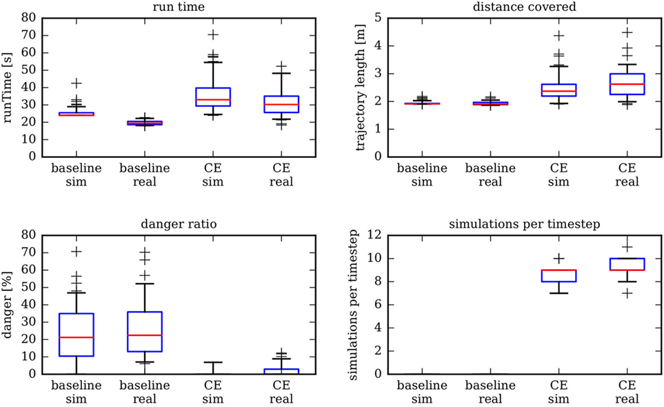
Figure 13. Statistical analysis for 88 simulations and 54 real robot experiments considering four basic metrics and comparing them to the baseline experiment. The box plots depict median, 25-quantile, and 75-quantile as a box. Whiskers depict 5-quantile and 95-quantile, and crosses depict data points outside those quantiles.
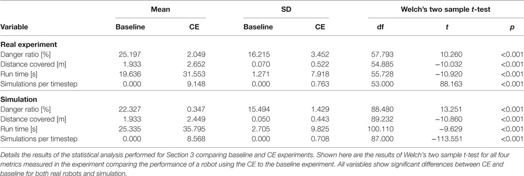
Table 1. Table of test statistics for the Welch’s two sample t-test for both experiment series testing for differences between baseline and CE experiment.
The first thing to notice is how remarkably close simulation and real world experiments are. The two main reasons for this are first that the simulator itself is very accurate and well calibrated to the real world robots (cf. Section 2.3.3) and second that there is almost no measurement noise in the system due to the high precision of the motion capture system used for virtual sensing. In a real application, estimating the pose of other robots using, for example, a camera system is a difficult task. Note that even though the differences between experiment and simulation are small, most of them are statistically significant (cf. Table 2 in Section 4.4). In particular, the differences between simulation and real experiments in the CE case are significant for all four metrics. This is to be expected as there are no simulations without a reality gap.
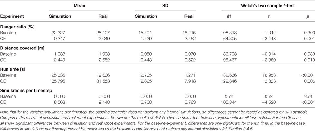
Table 2. Shown are test statistics for the Welch’s two sample t-test testing for differences between real experiment and simulation for all measured variables.
For the baseline experiment, the smart robot travels with maximum speed in a straight line from its start position to the goal and only diverts from its path for IR-based obstacle avoidance, which operates at a range of a few cm. As both speed and distance between start and goal are fixed, the resulting distributions of run time and distance covered show very little variance compared to the ones for the smart robot employing the CE mechanism.
As expected, the smart robot employing the CE mechanism takes more time to reach its goal and covers more distance doing so. The increase is moderate and it is about 50% more time used and 30% more distance covered. Those are not symmetrical since the robot can also stop and thus take longer to reach its goal without traveling further. Furthermore, variance in the results is increased for the smart robot, which is also to be expected.
The smart robot using the CE mechanism is much safer. In simulation, it is almost perfectly safe but the improvement in the real experiments is still large. This result is due to the fact that in pure simulation the simulated possible next actions are a direct continuation of the past trajectories, which were also simulated by the same simulator, as there is no reality gap (cf. Section 2.3.3). This improvement comes at the cost of having to perform the simulations with the corresponding computational cost, while the baseline robot can act with a purely reactive controller. Here, the trade-off between computational complexity and effectiveness between the two algorithms can be seen.
The danger ratio is a function of the safety distance parameter (cf. Section 2.2.1), which scales differently for the two controllers. For the baseline controller, the danger ratio increases almost linearly with the safety distance as a larger safety distance only increased the statistical chances of another robot being present inside of the safety area. For the smart robot running the CE, the function behaves more like a threshold function as it is able to avoid danger as long as the disk described by the safety distance can be maneuvered between the other robots for geometric reasons. For small safety distances, this is always possible, and for very large safety distances, for example, larger than the corridor width, this is impossible. The actual maximum safety distance which still allows the smart robot to move through the corridor depends on the density of the other robots and the corridor width. In a preliminary parameter study (not shown here), a safety distance of 0.2 m was identified experimentally as being just below this threshold for the experimental configuration presented.
4. Discussion
4.1. Key Findings
The experiment presented here has shown that a robot can move quickly and safely through a corridor occupied by a number of moving h-robots acting as proxy-humans by employing a simulation-based internal model. The robot was able to leverage the predictive capabilities of this internal model to look ahead in time and asses the consequences of its own actions as well as those of other actors in order to discard dangerous actions before actually executing them. This way the robot was able to modify its own actions to ensure its safety as well as reach its goal. This strategy has been shown to be vastly more safe than a purely reactive strategy albeit at additional computational cost for the internal simulation. By aggressively managing the simulation budget available to the robot, a real-time implementation of this architecture has been shown to be feasible on a modern laptop computer.
Following Craik and later Holland who envisioned agents that employ an internal model to try out different alternative actions without having to commit to them (Craik, 1967; Holland, 1992), the robot can anticipate unsafe situations before they arise. In this sense, the robot running the CE can be seen as an (admittedly simplistic) implementation of a Popperian creature as conceptualized by Dennett (1995), showing in this experiment that being able to generate and test what-if hypotheses leads to safer behavior.
Furthermore, this experiment has shown how the CE can, with its internal simulation mechanism, take into account both second order effects, i.e., robots interacting with the environment—which in this experiment means interacting with the walls of the corridor—and third-order effects, i.e., robots interacting with other robots, in order to correctly assess the consequence of the smart robot’s actions. These third-order effects are typical in swarm scenarios where large numbers of robots are loosely coupled by their interactions. This goes far beyond simple avoidance of the other robots and could more correctly be classified as strategic behavior.
4.2. Related Work
4.2.1. Robots with Internal Models
There are two main kinds of internal models: forward models (predictors), which predict future sensory inputs as a consequence of given motor inputs, and inverse models (controllers), which supply motor commands leading to a desired sensory input (Wolpert et al., 1995). Additionally, there are models predicting physical properties of the environment (Flanagan et al., 2001; Zago et al., 2004). Together, these models can be used to generate and test hypotheses about the outcome, i.e., consequences, of possible future actions and can also be used to recognize the behavior of other agents.
In control theory, the use of internal models is well established in areas such a model-driven control (Garcia and Morari, 1982) or predictive control (Morari and Lee, 1999). In general, the idea is that the use of coupled forward models (predictors) and inverse models (controllers) can overcome problems of more complex motor tasks posed by sensor and motor delays. In fact, it has been shown that for certain classes of problems models are strictly necessary (Conant and Ross Ashby, 1970; Francis and Wonham, 1976). A similar idea is employed in recursive Bayesian estimation such as Kalman (Kalman, 1960) or particle filters (Liu and Chen, 1998) where each update step integrates predictions based on a model and prior knowledge of the state with measurements to generate output estimates of the state.
Anticipation can improve the performance of navigation in complex tasks, while for simple tasks, a purely reactive strategy can perform better than one using anticipation. Furthermore, it has been shown that the quality of the predictions is one of the deciding variables for this improvement (Johansson and Balkenius, 2006). A second important variable for the improvement in performance by anticipation is the amount of time predicted into the future, which has an optimum between not predicting far enough into the future and predicting too far (Johansson and Balkenius, 2008).
More recently, internal models and simulations have been used in developmental robotics inspired by models of human motor control with noise and delays (Wolpert and Kawato, 1998). Demiris and Khadhouri (2006) implemented internal models based on pairs of forward and inverse models for motor actions of a robot. Schillaci et al. implemented an internal model based on forward and inverse models learned during exploration behavior on a humanoid robot. The learned internal models were used for arm reaching behavior, tool-use (Schillaci et al., 2012a), and human behavior recognition (Schillaci et al., 2012b). A review on how internal simulations can be used as tools to model cognition in artificial agents can be found in Schillaci et al. (2016).
In contrast to developmental robotics, however, the internal models used in the context of control theory are typically mathematical systems of the system (the plant) and stated explicitly when designing the controller, for example, as systems of differential equations. In robotics, the goal is to have the robot learn the internal models—both the inverse and forward models—autonomously. An example of such a strategy would be self-exploration mediated through babbling (Der and Martius, 2006; Schillaci and Hafner, 2011; Baranes and Oudeyer, 2013; Martius et al., 2014).
Most internal (forward) models consider only short predictions into the future in a tight sensorimotor loop. Internal simulation goes further than that in the sense of being more complete—often also incorporating the environment—and by simulating further into the future. In principle, short predictive steps can be chained so there is no clear border between those two extremes. An investigation into multistep predictions can, for example, be found in Ziemke et al. (2005). Here, internal simulation is used only as a name for a more complicated internal prediction mechanisms.
An internal simulation can—together with the corresponding inverse models and the ability to generate and try out actions—provide a robot with a “functional imagination” (Marques and Holland, 2009).
The idea of using an actual simulator instead of learned models has also started to be explored in the field of robotics since the computational power of robots has been increasing steadily. For example, Bongard et al. (2006) show a four-legged robot that can use an explicit internal simulation for the tasks of self-modeling and action generation for locomotion. Using this architecture, the robot can recover from physical damage by re-learning its new self-model generating a new gait for the changed morphology. Similarly, a swarm of robots has been shown to be able to use internal simulation of the robot and its environment to evolve robot controllers, which are then used on the real robots (O’Dowd et al., 2011). This system has been shown to be able to adapt to changes in the environment. More recently, Millard et al. (2014a,b) explore the use of simulation-based internal models to detect faults in swarm robotics systems.
4.2.2. Safety (with Internal Models)
In physical human–robot interaction (pHRI), safety analysis and safe control of personal robots is a relatively understudied area. Some notable work in the field has come from the PHRIENDS project (Physical Human-Robot Interaction: Dependability and Safety) (Alami et al., 2006), which undertook an in-depth study of pHRI. The state-of-the-art approach involves a systematic design time hazards analysis, which seeks to identify all possible safety hazards so that appropriate safe responses can be designed into the robot’s control system. Hazards analysis typically uses methods such as Failure Modes and Effects Analysis (FMEA) or HAZard and OPerability studies (HAZOP) (Bahr, 1997). In Woodman et al. (2012), this approach was extended with a framework that derives a safety system from the hazards analysis, which is first used to verify that safety constraints have been implemented correctly then, at run time, serves as a high-level safety enforcer by governing the actions of the robot, and preventing the control system from performing unsafe operations.
A fundamental limitation of the design time hazards analysis approach to safety in pHRI is that it requires the designer to anticipate all possible safety hazards—including interactions with dynamic actors such as humans. For robots operating in more complex dynamic and unknown environments, this becomes very difficult and, as was suggested in Woodman et al. (2012), increasingly infeasible; indeed, that paper concluded that new approaches are needed, which identify safety hazards instead at run time. In this paper, we propose one such approach, using an internal self- and other simulator. As far as we are aware, this is the first work proposing simulation-based internal models for safety.
4.3. Limitations
The sensing task has been strongly simplified in this implementation by using an external tracking system as a virtual sensor for the robot. For a fully embodied implementation, this task has to be solved on the robot using sensors such as, for example, a camera. These tasks have in principle been solved to a large degree but these solutions are often computationally expensive so they compete with the internal simulation for the computational resources of the robot making a fully embodied implementation challenging.
Additionally, the internal models used by the internal simulation—forward models, i.e., body models and physical models, as well as inverse models, i.e., controllers and intentions/goals—are known a priori to the robot. In general, similar models have been shown to be learnable by robots, but are often less complex than the ones employed by the simulator. In particular, the details and precision of the Stage simulator used for the internal simulation cannot yet be matched by learned models. In respect to the motivating scenario of humans walking through a museum, this gap is particularly big. However, as discussed in Section 2.4, human behavior can sometimes be modeled by simple models such as, for example, for pedestrians on a sidewalk or in panic situations.
In this experiment, only one robot was running a CE. This implementation of a CE was not designed with the possibility of several robots running a CE at the same time in mind, as the simulator in simplified terms assumes ballistic movement for the other robots. If two robots were to run this CE at the same time, a situation similar to two pedestrians moving toward each other on a sidewalk would result where both oscillate back and forth between avoidance and movement toward the goal. In principle, this would result either in none of the robots being able to reach the goal or in an unsafe situation. However, as previous work on the CE has suggested (Winfield et al., 2014), noise is likely to break the symmetry of this situation resolving the dilemma naturally.
There are additional limitations of the internal simulation itself: the issue of the exploding search tree (cf. Section 2.3.2) when performing simulations has not been solved yet and in this work a greedy depth-first search has been employed. Without resolving this issue, this naive implementation will not scale well to other robots employing more complex behavior. However, scaling to situations with many more robots with the same robot controllers as used in the experiment is straightforward, as the penalty on the simulation budget is minimal because of the good scaling properties of the Stage simulator (Vaughan, 2008).
Despite these limitations, the use of simulation-based internal models for safety in dynamic environments has proven to be very successful. Therefore, further exploring this approach holds promise for robot safety in pHRI scenarios. Possible future work resulting from this discussion is presented in Section 4.4.
4.4. Outlook and Future Work
There are four main possible avenues for potential future work. The most obvious avenue would be to use more complex robots instead of minimalistic e-puck robots to increase the number of free parameters and complexity in order to test the limits of the simulation tools and sensing in regard of the reality gap. This not only means more complex bodies and dynamics but also more complex controllers and behavior of the robots. This would also be a first step away from simple robots representing humans walking on the sidewalk while not paying attention—who can be avoided without them even realizing that they have been avoided—toward a more realistic HRI scenario.
Additionally, for actual embodied implementations, the sensing also has to be embodied so the OTL has to be implemented using the sensory modalities of the robot such as, for example, a camera instead of an external tracking system. Furthermore, the a priori existing internal simulator as used in this experiment has to be replaced by learned internal models of the environment and the other robots/agents. And finally, the last big open question is how the challenge of the exploding search tree can be solved. One interesting option for that would be to use a particle filter such as Markov chain Monte Carlo probability density estimation instead of using single discretized actions.
Author Contributions
This work is based on the original idea by AW for the concept of the CE and the work presented in Winfield et al. (2014). The experiment as well as the analysis was implemented, designed, and performed by CB. The creation of the text was a joint effort of all authors.
Conflict of Interest Statement
The authors declare that the research was conducted in the absence of any commercial or financial relationships that could be construed as a potential conflict of interest.
Acknowledgments
The authors thank Dr. Wenguo Liu (Bristol Robotics Laboratory) for his invaluable assistance with the physical robots and the general experimental setup. The authors also thank Dr. Andy Radford (University of Bristol) for discussions and his advice in designing the experiment in order to mitigate the effects of inter-robot homogeneity. This paper is based on the PhD Thesis of Christian Blum (Blum, 2015).
Funding
This research was supported by the German Academic Exchange Service (DAAD) and the Deutsche Forschungsgemeinschaft (DFG) grant HA 5458/9-1.
Supplementary Material
The Supplementary Material for this article can be found online at http://www.frontiersin.org/articles/10.3389/frobt.2017.00074/full#supplementary-material.
Figure S1. Exemplary run number 1 of the corridor scenario experiment showing only the performance of the CE controller.
Figure S2. Exemplary run number 2 of the corridor scenario experiment showing only the performance of the CE controller.
Figure S3. Exemplary run number 3 of the corridor scenario experiment showing only the performance of the CE controller.
Figure S4. Exemplary run number 4 of the corridor scenario experiment showing only the performance of the CE controller.
Figure S5. Exemplary run number 5 of the corridor scenario experiment showing only the performance of the CE controller.
Footnotes
- ^Walls are not considered as obstacles in this specific sense.
- ^In the actual implementation, not all grid points are sampled at all times, instead the attention radius mechanism (cf. section 2.3.5) restricts the grid points sampled. In practice, this means that on average, around half of the grid points are sampled (cf. Figure 13, which shows that on average around 10 simulations are executed per time step).
- ^This effect is probably due to the response of the virtual IR sensor being too weak. However, it proved impossible to at the same time reproduce correct trajectories and eliminate this effect.
- ^Lenovo T440s, Intel i5 4200 @ 1.6 GHz, 12 GB RAM.
- ^Vicon Motion Systems Ltd., http://www.vicon.com/.
- ^https://code.google.com/p/protobuf/.
- ^Lenovo T440s, Intel i5 4200 @ 1.6 GHz, 12 GB RAM.
References
Alami, R., Albu-Schaeffer, A., Bicchi, A., Bischoff, R., Chatila, R., De Luca, A., et al. (2006). “Safe and dependable physical human-robot interaction in anthropic domains: state of the art and challenges,” in 2006 IEEE/RSJ International Conference on Intelligent Robots and Systems (Beijing: IEEE), 1–16.
Bahr, N. (1997). System Safety Engineering and Risk Assessment: A Practical Approach. Chemical Engineering. Washington, DC: Taylor & Francis.
Baranes, A., and Oudeyer, P.-Y. (2013). Active learning of inverse models with intrinsically motivated goal exploration in robots. Rob. Auton. Syst. 61, 49–73. doi: 10.1016/j.robot.2012.05.008
Blum, C. (2015). Self-Organization in Networks of Mobile Sensor Nodes. Ph.D. thesis. Berlin: Humboldt-Universität zu Berlin, Mathematisch-Naturwissenschaftliche Fakultät.
Bongard, J., Zykov, V., and Lipson, H. (2006). Resilient machines through continuous self-modeling. Science 314, 1118–1121. doi:10.1126/science.1133687
Conant, R. C., and Ross Ashby, W. (1970). Every good regulator of a system must be a model of that system? Int. J. Syst. Sci. 1, 89–97. doi:10.1080/00207727008920220
Demiris, Y., and Khadhouri, B. (2006). Hierarchical attentive multiple models for execution and recognition of actions. Rob. Auton. Syst. 54, 361–369. doi:10.1016/j.robot.2006.02.003
Der, R., and Martius, G. (2006). “From motor babbling to purposive actions: emerging self-exploration in a dynamical systems approach to early robot development,” in From Animals to Animats 9, eds S. Nolfi, G. Baldassarre, R. Calabretta, J. C. T. Hallam, D. Marocco, J-A. Meyer, et al. (Springer), 406–421.
Echeverria, G., Lassabe, N., Degroote, A., and Lemaignan, S. (2011). “Modular open robots simulation engine: Morse,” in 2011 IEEE International Conference on Robotics and Automation (ICRA) (Shanghai: IEEE), 46–51.
Flanagan, J. R., King, S., Wolpert, D. M., and Johansson, R. S. (2001). Sensorimotor prediction and memory in object manipulation. Can. J. Exp. Psychol. 55, 87. doi:10.1037/h0087355
Francis, B. A., and Wonham, W. M. (1976). The internal model principle of control theory. Automatica 12, 457–465. doi:10.1016/0005-1098(76)90006-6
Garcia, C. E., and Morari, M. (1982). Internal model control. a unifying review and some new results. Ind. Eng. Chem. Process Des. Dev. 21, 308–323. doi:10.1021/i200017a016
Haruno, M., Wolpert, D., and Kawato, M. (2001). Mosaic model for sensorimotor learning and control. Neural Comput. 13, 2201–2220. doi:10.1162/089976601750541778
Helbing, D., Farkas, I., and Vicsek, T. (2000). Simulating dynamical features of escape panic. Nature 407, 487–490. doi:10.1038/35035023
Helbing, D., and Molnar, P. (1995). Social force model for pedestrian dynamics. Phys. Rev. E 51, 4282. doi:10.1103/PhysRevE.51.4282
Hesslow, G. (2002). Conscious thought as simulation of behaviour and perception. Trends Cogn. Sci. 6, 242–247. doi:10.1016/S1364-6613(02)01913-7
Hesslow, G. (2012). The current status of the simulation theory of cognition. Brain Res. 1428, 71–79. doi:10.1016/j.brainres.2011.06.026
Jacobi, N., Husbands, P., and Harvey, I. (1995). “Noise and the reality gap: the use of simulation in evolutionary robotics,” in Proceedings of the Third European Conference on Advances in Artificial Life (Berlin: Springer), 704–720.
Johansson, B., and Balkenius, C. (2006). “An experimental study of anticipation in simple robot navigation,” in Workshop on Anticipatory Behavior in Adaptive Learning Systems (Berlin: Springer), 365–378.
Johansson, B., and Balkenius, C. (2008). “Prediction time in anticipatory systems,” in Workshop on Anticipatory Behavior in Adaptive Learning Systems (Berlin: Springer), 283–300.
Kalman, R. E. (1960). A new approach to linear filtering and prediction problems. J. Fluids Eng. 82, 35–45.
Koenig, N., and Howard, A. (2004). “Design and use paradigms for gazebo, an open-source multi-robot simulator,” in Proceedings of the 2004 IEEE/RSJ International Conference on Intelligent Robots and Systems, 2004 (IROS 2004), Vol. 3 (Sendai: IEEE), 2149–2154.
Liu, J. S., and Chen, R. (1998). Sequential Monte Carlo methods for dynamic systems. J. Am. Stat. Assoc. 93, 1032–1044. doi:10.1080/01621459.1998.10473765
Liu, W., and Winfield, A. F. T. (2011). Open-hardware e-puck Linux extension board for experimental swarm robotics research. Microprocess. Microsyst. 35, 60–67. doi:10.1016/j.micpro.2010.08.002
Marques, H. G., and Holland, O. (2009). Architectures for functional imagination. Neurocomputing 72, 743–759. doi:10.1016/j.neucom.2008.06.016
Martius, G., Jahn, L., Hauser, H., and Hafner, V. V. (2014). “Self-exploration of the stumpy robot with predictive information maximization,” in From Animals to Animats 13, volume 8575 of Lecture Notes in Computer Science, eds A. P. del Pobil, E. Chinellato, J. Martinez-Martin, E. Hallam, E. Cervera, and A. Morales (Cham: Springer International Publishing), 32–42.
Michel, O. (2004). Webots: professional mobile robot simulation. Int. J. Adv. Robot. Syst. 1, 39–42. doi:10.5772/5618
Millard, A. G., Timmis, J., and Winfield, A. F. (2014a). “Run-time detection of faults in autonomous mobile robots based on the comparison of simulated and real robot behaviour,” in 2014 IEEE/RSJ International Conference on Intelligent Robots and Systems (IROS 2014) (Chicago, IL: IEEE), 3720–3725.
Millard, A. G., Timmis, J., and Winfield, A. F. (2014b). “Towards exogenous fault detection in swarm robotic systems,” in Towards Autonomous Robotic Systems (Berlin: Springer), 429–430.
Mischiati, M., Lin, H.-T., Herold, P., Imler, E., Olberg, R., and Leonardo, A. (2015). Internal models direct dragonfly interception steering. Nature 517, 333–338. doi:10.1038/nature14045
Mondada, F., Bonani, M., Raemy, X., Pugh, J., Cianci, C., Klaptocz, A., et al. (2009). “The e-puck, a robot designed for education in engineering,” in Proceedings of the 9th Conference on Autonomous Robot Systems and Competitions, number LIS-CONF-2009-004 (IPCB: Instituto Politécnico de Castelo Branco), 59–65.
Morari, M., and Lee, J. H. (1999). Model predictive control: past, present and future. Comput. Chem. Eng. 23, 667–682. doi:10.1016/S0098-1354(98)00301-9
Musse, S. R., and Thalmann, D. (1997). A Model of Human Crowd Behavior: Group Inter-Relationship and Collision Detection Analysis. Vienna: Springer.
O’Dowd, P. J., Winfield, A. F. T., and Studley, M. (2011). “The distributed co-evolution of an embodied simulator and controller for swarm robot behaviours,” in Proceedings of the IEEE/RSJ International Conference on Intelligent Robots and Systems (IROS), San Francisco, CA, 4995–5000.
Schillaci, G., and Hafner, V. V. (2011). “Random movement strategies in self-exploration for a humanoid robot,” in Proceedings of the 6th International Conference on Human-Robot Interaction (New York, NY: ACM), 245–246.
Schillaci, G., Hafner, V. V., and Lara, B. (2012a). “Coupled inverse-forward models for action execution leading to tool-use in a humanoid robot,” in Proceedings of the Seventh Annual ACM/IEEE International Conference on Human-Robot Interaction (New York, NY: ACM), 231–232.
Schillaci, G., Lara, B., and Hafner, V. V. (2012b). “Internal simulations for behaviour selection and recognition,” in Human Behavior Understanding, volume 7559 of Lecture Notes in Computer Science (Berlin: Springer), 148–160.
Schillaci, G., Hafner, V. V., and Lara, B. (2016). Exploration behaviors, body representations, and simulation processes for the development of cognition in artificial agents. Front. Robot. AI 3:39. doi:10.3389/frobt.2016.00039
Spears, W., and Spears, D. (2012). Physicomimetics: Physics-Based Swarm Intelligence. Berlin Heidelberg: Springer.
Vanderelst, D., and Winfield, A. (2017). An architecture for ethical robots inspired by the simulation theory of cognition. Cogn. Syst. Res. Elsevier. doi:10.1016/j.cogsys.2017.04.002
Vaughan, R. (2008). Massively multi-robot simulation in stage. Swarm Intell. 2, 189–208. doi:10.1007/s11721-008-0014-4
Vaughan, R. T., and Gerkey, B. P. (2007). “Really reused robot code from the player/stage project,” in Software Engineering for Experimental Robotics, ed. D. Brugali (Berlin: Springer), 267–289.
Winfield, A. (2014). “Robots with internal models: a route to self-aware and hence safer robots,” in The Computer After Me: Awareness And Self-Awareness In Autonomic Systems, ed. J. Pitt (London: Imperial College Press), 237–252.
Winfield, A. F. T., Blum, C., and Liu, W. (2014). “Towards an ethical robot: internal models, consequences and ethical action selection,” in Advances in Autonomous Robotics Systems, eds M. Mistry, A. Leonardis, M. Witkowski, and C. Melhuish (Springer), 85–96.
Wolpert, D. M., Diedrichsen, J., and Flanagan, J. R. (2011). Principles of sensorimotor learning. Nat. Rev. Neurosci. 12, 739–751. doi:10.1038/nrn3112
Wolpert, D. M., Ghahramani, Z., and Jordan, M. I. (1995). An internal model for sensorimotor integration. Science 269, 1880–1882. doi:10.1126/science.7569931
Wolpert, D. M., and Kawato, M. (1998). Multiple paired forward and inverse models for motor control. Neural Netw. 11, 1317–1329. doi:10.1016/S0893-6080(98)00066-5
Woodman, R., Winfield, A. F., Harper, C., and Fraser, M. (2012). Building safer robots: safety driven control. Int. J. Robot. Res. 31, 1603–1626. doi:10.1177/0278364912459665
Zago, M., Bosco, G., Maffei, V., Iosa, M., Ivanenko, Y. P., and Lacquaniti, F. (2004). Internal models of target motion: expected dynamics overrides measured kinematics in timing manual interceptions. J. Neurophysiol. 91, 1620–1634. doi:10.1152/jn.00862.2003
Keywords: robot safety, multi-robot systems, swarm robotics, internal modeling, internal simulations
Citation: Blum C, Winfield AFT and Hafner VV (2018) Simulation-Based Internal Models for Safer Robots. Front. Robot. AI 4:74. doi: 10.3389/frobt.2017.00074
Received: 02 September 2017; Accepted: 15 December 2017;
Published: 11 January 2018
Edited by:
Daniel Polani, University of Hertfordshire, United KingdomCopyright: © 2018 Blum, Winfield and Hafner. This is an open-access article distributed under the terms of the Creative Commons Attribution License (CC BY). The use, distribution or reproduction in other forums is permitted, provided the original author(s) or licensor are credited and that the original publication in this journal is cited, in accordance with accepted academic practice. No use, distribution or reproduction is permitted which does not comply with these terms.
*Correspondence: Christian Blum, blum@informatik.hu-berlin.de